Deterministic Mean-field Ensemble Kalman Filtering

Abstract

The proof of convergence of the standard ensemble Kalman filter (EnKF) from Legland etal. 2011 [39] is extended to non-Gaussian state space models. A density-based deterministic approximation of the mean-field limit EnKF (DMFEnKF) is proposed, consisting of a PDE solver and a quadrature rule. Given a certain minimal order of convergence $\kappa$ between the two, this extends to the deterministic filter approximation, which is therefore asymptotically superior to standard EnKF for dimension $d<2\kappa$. The fidelity of approximation of the true distribution is also established using an extension of total variation metric to random measures. This is limited by a Gaussian bias term arising from non-linearity/non-Gaussianity of the model, which arises in both deterministic and standard EnKF. Numerical results support and extend the theory.

1 Introduction

The filtering problem, referred to in the geophysical community as data assimilation [33], consists of obtaining meaningful information sequentially online about a signal evolving in time, given noisy observations of that signal. From the Bayesian perspective the solution of the filtering problem is given by the posterior distribution of the signal given all the previous observations [30, 4, 31, 57, 2]. The signal is typically modeled by a Markov process in which the observation at a given time is conditionally independent upon the rest of the observations given the observed state at that time. This set-up is then referred to as a hidden Markov model [14]. In the case of linear Gaussian state-space model, the solution is also Gaussian, and therefore it can be parametrized by its mean and covariance and is given exactly in closed form by the Kalman filter [32]. In general, other cases must be treated non-parametrically, for example with computational algorithms. The optimal filter is a point estimator given by the expected value of the filtering distribution [30, 4]. This can be estimated consistently using particle filtering algorithms [4, 19, 20]. Indeed the particle filter consistently approximates any quantity of interest, i.e. any conditional expectation. Despite being asymptotically consistent in the large particle limit, it is well-known that the accuracy of particle filters is hindered by a constant that grows exponentially with dimension [6, 50]. Furthermore, naive bounds indicate the constant may also grow with time, however if the hidden process has a Dobrushin ergodic coefficient [18] then a uniform-in-time estimate can be obtained [17]. In the geophysical community, the dimension of the state-space is typically enormous, and so practitioners have resorted to sub-optimal filters such as the ensemble Kalman filter (EnKF) [26] and its incarnations. It has been shown by [39, 35, 43] that some versions of EnKF for models of a particular class converge to a mean-field limit, which is defined herein as a process in which the current state depends only on the previous state and the statistics of the process. Such filters may perform well in high dimensions for small ensembles, but are biased in the sense that the mean-field limiting distribution is not the filtering distribution and so estimators of quantities of interest do not converge to the correct value in the large ensemble limit. As both of these methods depend on random ensembles of particles, the asymptotic approximation error of expectations with respect to their respective limits is given by $\mathcal{O}(N^{-1/2})$ for an ensemble size $N$. Interestingly, it has been observed that the signal-tracking error of EnKF may not decrease for ensembles larger than 50-100 for the quasi-geostrophic equations in [26], indicating the error may become dominated by the bias arising from the linearity assumption.

The EnKF is a filtering algorithm which was introduced in [26] and later corrected in [13]. Herein the filter is developed from the perspective as a Monte-Carlo approximation of the minimum mean-square error linear estimator (Thm. 1, p. 87 and Thm. 3, p. 92 of [41]). For a single step in the mean-field limit (ensemble size $N\rightarrow\infty$), EnKF returns a random variable whose expected value has the minimum mean-square error over all estimators of the forecasted signal which are linear in the new observation. Furthermore, this random variable has as its covariance the error covariance between the minimum mean-square error linear estimator and the truth. It can thus be viewed as a best linear approximation of the target for a single step. It is of course not the unique random variable with this mean and covariance, even among those which are linear in the observation. For linear Gaussian models however, this estimator happens to be the mean of the posterior distribution, which is given by a single step of the Kalman filter [32]. Furthermore, in this case the error covariance of the estimator is the covariance of the posterior distribution. Hence the corresponding random variable is distributed according to the filtering distribution, and this holds for all time. The mean of the posterior filtering distribution is the minimum mean-square error estimator over all square integrable functions of the observation, and is hence known as the optimal filter [30]. For nonlinear and/or non-Gaussian models linear estimators based on the procedure outlined above do not yield the mean of the updated posterior filtering distribution, which is in general nonlinear in the observations. Therefore, in this case linear estimators correspond to sub-optimal filters. The theory above was translated into finite-resolution approximations of sub-optimal filters using ensemble approximations in the EnKF algorithm [13], and using random-variable-based deterministic approximations in the algorithms of [48, 40, 23] and references therein. The papers [3, 10] caution against the use of random-variable expansions for the forward propagation of uncertainty. While the mean-field EnKF yields a non-Gaussian approximation, the mean and covariance are identical to those obtained by making a Gaussian approximation of the forecast distribution and updating that Gaussian with the Gaussian observations, as done for example in [56]. Such procedure would therefore also yield a best linear approximation for a single step as defined above. The results herein will illustrate that the EnKF estimator may actually perform better than such Gaussian approximation in recovering the mean and covariance in the long-run.

Great effort has been invested in approximating the filtering distribution using particle and ensemble methods [19, 59, 16, 54, 51, 29, 1], while decidedly less attention has been invested in deterministic approximations [27, 42, 53, 21, 22, 48, 40, 5]. The idea of numerically approximating the evolution of the Fokker-Planck equation and imposing the update by multiplication and normalization in the continuous-discrete setting has been done in the works [27, 42]. It was used in those works, as it will be here, as a benchmark against which to evaluate other algorithms developed. Here referred to as the full Fokker Planck filter (FPF), it is actually also advocated as a legitimate and competitive method which can be lifted to higher-dimensional problems using sparse-grid parametrization ideas (see, for example, [12, 5]). More sophisticated approximations of the density should be capable of handling much higher dimensions. Furthermore, it is well-known that very high-dimensional models may exhibit nonlinearity/instability/non-Gaussianity only on low-dimensional manifolds [11, 7, 15, 55, 28, 58, 37]. Therefore, it is conceivable that the space can be decomposed, and such approximation of the true filtering distribution may be used on the unstable space, while a simpler filter (e.g. ensemble or extended Kalman or even 3DVAR) may be used on the complement. In certain cases such approaches may be particularly simple. For example, in a particular context of Lagrangian data assimilation it has been proposed to use a particle filter on the flow state and the Fokker-Planck equation for the evolution of observed passive tracers, which are conditionally independent given a particular flow state [53].

The aim of this work is two-fold: first, a deterministic approach to solving the mean-field EnKF (MFEnKF) via accurate numerical approximation of the Fokker-Planck equation is proposed, and the analogous approximation of the true filter, FPF [27, 42], is used as a benchmark against which to evaluate other filters numerically, in particular the standard EnKF and deterministic EnKF (DMFEnKF). The DMFEnKF is not proposed here as an alternative to the Full FPF, as the latter will provably always have lower mean square error (MSE) for sufficiently accurate approximation schemes. However, the DMFEnKF may be more robust to errors, as it replaces the normalization step of the Full FPF by a linear change of variables and convolution with a Gaussian density. Second, the convergence rates of the standard EnKF and DMFEnKF to the MFEnKF are derived. It is shown that the latter has a faster asymptotic rate of convergence than the former for $d<2\kappa$, where $\kappa$ is the minimal rate of convergence of the numerical approximation of the Fokker-Planck equation and the quadrature rule for $d=1$. In short, the order of convergence of the standard density and quadrature approximations extends to the filtering density approximation for finite times. It is also proven that the value of this faster convergence is limited by the Gaussian bias of the MFEnKF when the underlying nonlinearity/non-Gaussianity of the forward model becomes significant, for example from longer integration of a nonlinear SDE between observations. In this case, the approximation of the true filter may be used as an accurate and effective algorithm also for $d<2\kappa$, although this is not emphasized in the present work. The theoretical results are complemented by numerical experiments which confirm the theory and also illustrate exactly where the Gaussian error is greatest. In particular, approximating the forecast distribution by a Gaussian gives a less accurate approximation than standard mean-field EnKF, while approximating the updated distribution by a Gaussian after the full nonlinear update gives a more accurate approximation. The results of this paper complement recent results for the non-divergence, in terms of tracking the true signal, of continuous-discrete and continuous-continuous EnKF for a general class of quadratic-dissipative, noise-free, and possibly infinite-dimensional dynamics [34], which may be viewed as a particular class of nonlinear Gaussian state-space model (i.e. the case of degenerate dynamics in which the Fokker-Planck evolution in finite dimensions would reduce to Liouville equation for the continuous-discrete case). The results also complement recent results on convergence of EnKF to MFEnKF, for both the linear [35, 43] and nonlinear [39] Gaussian state-space model cases, by extending those results to the more general non-Gaussian case considered here and considering for the first time, to the knowledge of the authors, the fidelity with which MFEnKF approximates the true filtering distribution.

The rest of the paper will be structured as follows. In Section 2 the filtering problem is introduced and definitions of various notions of its solution are given and discussed. In Section 3 the ensemble Kalman filter is defined and related to the discussion of Section 2. In Section 4 the Fokker-Planck solution approach is introduced, several algorithms are defined, and the convergence theorem is presented. In Section 5 the majority of the theoretical results are presented. In Section 6 numerical experiments are done with the algorithms to confirm and extend the theoretical results. Finally, Section 7 gives conclusions and future directions.

2 Filtering

In this section a general filtering problem is set up and the meaning of solution is defined and discussed. In particular, the filtering distribution is introduced, which has the so-called optimal filter as its mean. Then suboptimal filters are introduced, including the set of one-step optimal linear filters, and some standard sub-optimal filters for general nonlinear Gaussian state-space models. The relation between the latter is highlighted, and this gives segue to the EnKF which will be the focal sub-optimal filter of this work.

2.1 Set-up

Throughout for any positive-definite $A\in\mathbb{R}^{\ell\times\ell}$, we introduce the following notations for weighted Mahalanobis inner-product $\langle\cdot,\cdot\rangle_{A}=\langle A^{-\frac{1}{2}}\cdot,A^{-\frac{1}{2}}\cdot\rangle$ and the resulting norm $|\cdot|_{A}=|A^{-\frac{1}{2}}\cdot|.$

Let $\mathcal{K}:\mathbb{R}^{d}\times\sigma(\mathbb{R}^{d})\to\mathbb{R}_{+}$ be a generic Markov kernel, where $\sigma(\mathbb{R}^{d})$ is the sigma algebra of measurable subsets of $\mathbb{R}^{d}$. This simultaneously gives rise to a linear operator on measures/densities and functionals so that for $f:\mathbb{R}^{d}\rightarrow\mathbb{R}$, $(\mathcal{K}f)(u)=\int_{\mathbb{R}^{d}}\mathcal{K}(u,dv)f(v)$, and for $\mu:\sigma(\mathbb{R}^{d})\rightarrow[0,1]$ with density $\rho:\mathbb{R}^{d}\rightarrow\mathbb{R}_{+}$, $\mu^{\prime}$ is a measure with density $\rho^{\prime}$ such that $\mu^{\prime}(A)=\int_{\mathbb{R}^{d}}\mu(du)\mathcal{K}(u,A)=\int_{\mathbb{R}^{d}}\rho(u)\mathcal{K}(u,A)du=\int_{A}\int_{\mathbb{R}^{d}}\rho(u)\mathcal{K}(u,v)dudv$ for all $A\in\sigma(\mathbb{R}^{d})$. This will be written as $\mu^{\prime}=\mathcal{K}^{\top}\mu$ or $\rho^{\prime}=\mathcal{K}^{\top}\rho$. This work will only concern distributions which have density with respect to Lebesgue measure and, as such, densities will be used interchangeably with probability measures. In particular, for each $u\in\mathbb{R}^{d}$, the measure $\mathcal{K}(u,\cdot)$ is simultaneously identified with its density $\mathcal{K}(u,v)$. Consider the Markov chain $u=\{u_{j}\}_{j\geq 0}$ defined by

$$u_{j+1} \sim \mathcal{K}(u_{j},\cdot),\;j=0,1,2,\dots,$$ (1)

$$u_{0} \sim \rho_{0}.$$

This Markov Chain returns a sequence of random variables related by the Markov property, i.e. $u_{k}|u_{j}=u_{k}|u_{j},u_{j-1},\dots,u_{0}$ for all $k>j$.

In many applications, models such as (1) are supplemented by observations of the system as it evolves. As part of the statistical model under consideration in the present work it is assumed that the data is defined as

$$y_{j}=Hu_{j}+\eta_{j},\;j=1,2,\dots,$$ (2)

where $H:\mathbb{R}^{d}\to\mathbb{R}^{m}$ is linear and $\eta=\{\eta_{j}\}_{j\geq 1}$ is an i.i.d. sequence, independent of $u_{0}$ and the noise in $\mathcal{K}$, with $\eta_{1}\sim N(0,\Gamma)$. The accumulated data is denoted $Y_{k}=\{y_{j}\}_{j=1}^{k}$. The objective of filtering is to determine information about the conditional, or filtered random variable $u_{j}|Y_{j}$. Its distribution is referred to as the filtering distribution and recovering either this distribution, or (ambiguously) even just an estimate of it, is referred to as filtering. We will refer to the former problem as the true filtering problem. Often the dependence on $u_{0}$ is neglected. This is reasonable in the case that the true filtering problem is stable, in the sense of forgetting its initial distribution in the large time limit.

Notice that models of the form (1) include models of the following form as a special case

$$u_{j+1} = \Psi(u_{j})+\xi_{j},\;j=0,1,2,\dots,$$ (3)

$$u_{0} \sim \rho_{0},$$

where $\Psi:\mathbb{R}^{d}\to\mathbb{R}^{d}$, and $\xi=\{\xi_{j}\}_{j\geq 0}$ is an i.i.d. sequence, independent of $u_{0}$, with $\xi_{0}\sim N(0,\Sigma)$. Gaussian state-space models of the form (3) are commonly encountered, in particular in the data assimilation community.

2.2 Filtering distribution

The true distribution of $u_{j}|Y_{j}$, which is our gold standard, has a recursive structure under the given assumptions. Define the unnormalized joint likelihood density $g(u,y)\propto p(y|u)$, for a particular pair $(u,y)$, as

$$g(u,y)=e^{-\frac{1}{2}|y-Hu|^{2}_{\Gamma}},$$ (4)

with shorthand $g_{j}(u)=g(u,y_{j})$. Furthermore define $\mathcal{C}_{j}$ as the nonlinear operator which updates the density according to the $j^{th}$ observation, i.e. for $u\sim\hat{\rho}$, $u|y_{j}\sim\rho$, where

$$\rho=\mathcal{C}_{j}\hat{\rho}:=\frac{\hat{\rho}g_{j}}{\int\hat{\rho}g_{j}}.$$ (5)

Notice that this operation is treacherous because either large or small values of $e^{-\frac{1}{2}|y-Hu|^{2}_{\Gamma}}$ can cause large error growth. In particular, $e^{-\frac{1}{2}|y-Hu|^{2}_{\Gamma}}$ is bounded below only by zero, although it obtains arbitrarily small values arbitrarily rarely, so the probability of the denominator being very small and leading to large amplification of errors is not high.

Denote the filtering density given $j$ observations by $\rho_{j}$, and then the recursion may be given by

$$\;\;\mbox{Forecast}\;\begin{array}[]{l}\hat{\rho}_{j}=\mathcal{K}^{\top}\rho_{j-1},\end{array}$$

$$\mbox{Update}\;\;\;\begin{array}[]{llll}\rho_{j}=\mathcal{C}_{j}\hat{\rho}_{j},\end{array}$$

where $\mathcal{K}$ is defined in (1). Or, in other words $\rho_{j}=\mathcal{C}_{j}\mathcal{K}^{\top}\rho_{j-1}$. In the following section we will derive a deterministic solution approach to approximating this recursion.

2.3 Optimal filtering

In the sense of mean-square error, the optimal point estimator $\hat{u}_{j}(Y_{j})$ (as a function of the observations) of the signal $u_{j}$ is $\mathbb{E}(u_{j}|Y_{j})$ [30, 8, 49, 23]. In other words

$$\mathbb{E}(u_{j}|Y_{j})={\rm argmin}_{\{\hat{u}=\phi(Y_{j});\phi\in L^{2}\}}\mathbb{E}|\hat{u}-u_{j}|^{2},$$ (6)

where the expectation is with respect to $(u_{j},Y_{j})$, and $L^{2}$ here denotes the collection of functions $f$ such that $\mathbb{E}_{Y}(f^{2}(Y)),$ where $\mathbb{E}_{Y}$ denotes expectation with respect to $Y$. A short concise proof of this fact may be found in Theorem 5.3 of [30]. The scrupulous reader may find more satisfaction in the exposition of [8] Theorem 3.2.6, a consequence of the Doob-Dynkin Lemma 2.1.24. Note $u_{j}\in L^{2}$ under mild assumptions on the kernel $\mathcal{K}$ and initial distribution [46], which will indeed be made later on. The optimal point estimator is a random variable for $Y_{j}$ random, and a deterministic variable for a given realization of $Y_{j}$. Our aim is to solve the true filtering problem, i.e. obtain the full filtering distribution of $u_{j}|Y_{j}$. It is nonetheless good to know that the optimal point estimator may be easily obtained from the true filtering distribution.

Naturally the fidelity with which we approximate $u_{j}|Y_{j}$ will dictate the fidelity with which we approximate (6). Assume one has access to the random variable $u_{j}|Y_{j-1}$ in the complete distributional sense. Then, upon conditioning the equation (2) on $Y_{j-1}$, one finds that $y_{j}|Y_{j-1}=Hu_{j}|Y_{j-1}+\eta_{j}$. Therefore (6) can also be represented in terms of the one-step optimal point estimator, following Doob-Dynkin, where

$$\mathbb{E}(u_{j}|Y_{j})=\mathbb{E}[(u_{j}|Y_{j-1})|(y_{j}|Y_{j-1})]={\rm argmin}_{\{\hat{u}=\phi(y_{j}|Y_{j-1});\phi\in L^{2}\}}\mathbb{E}|\hat{u}-(u_{j}|Y_{j-1})|^{2}.$$ (7)

In other words, the minimum mean-square error estimator of the time $j$ state given the time $j-1$ filtering distribution and the $j^{th}$ observation is the expectation of the time $j$ filtering distribution, as expected. This of course requires knowing the full (filtering) distribution of $u_{j-1}|Y_{j-1}$ to get the (forecast) distribution of $u_{j}|Y_{j-1}$. In fact, one finds that the formula for $\mathbb{E}(u_{j}|Y_{j})$ only relies on $\mathbb{E}(u_{j}|Y_{j-1})$ in the linear case (c.f. Thm. 3, p. 92 [41]).

2.4 Sub-optimal filtering

The optimal filter is often very difficult to obtain, particularly in high-dimensional problems. So in practice one may resort to sub-optimal filters. We present the one-step optimal linear filter for general models, which only uniquely defines mean and covariance.

2.4.1 One-step optimal linear filter

Given the distribution of $u_{j}|Y_{j-1}$, obtaining even the one-step optimal point estimator (7) is often a formidable task for high-dimensional models, so one may consider instead the one-step optimal linear point estimator defined as the best estimator $\hat{u}=\phi(y_{j}|Y_{j-1})$ out of the class of linear functions $\phi(y)=Ky+b$ (Thm. 1, p. 87 [41]). In the remainder of discussion here all random variables are conditioned on $Y_{j-1}$ and the conditional dependence is omitted to avoid notational clutter. The following optimization problem is solved

$$m_{j}(y_{j})={\rm argmin}_{\left\{\hat{u}=\phi(y_{j});\phi(y)~{}{\rm linear}\right\}}\mathbb{E}|\hat{u}-u_{j}|^{2}.$$ (8)

Let $\phi(y)=K_{j}y+b_{j}$, and let $y_{j}=Hu_{j}+\eta_{j}$ be the random variable defined in (2). Optimizing this equation with respect to $K_{j}$ and $b_{j}$ gives [41]

$$K_{j} =\mathbb{E}[(u_{j}-\mathbb{E}u_{j})\otimes(y_{j}-\mathbb{E}y_{j})]\mathbb{E}[(y_{j}-\mathbb{E}y_{j})\otimes(y_{j}-\mathbb{E}y_{j})]^{-1},$$ (9)

$$m_{j}(y_{j}) =\mathbb{E}u_{j}+K_{j}(y_{j}-H\mathbb{E}u_{j}).$$ (10)

Notice that $\mathbb{E}m_{j}=\mathbb{E}u_{j}$, but indeed it is not necessarily the case that $m_{j}=\mathbb{E}(u_{j}|y_{j})$. In fact, this is only the case when $u_{j}$ is Gaussian. Note that this holds only while $y_{j}$ is a random variable. In practice, for the quenched case, in which $y_{j}$ is a deterministic realization, $m_{j}$ is deterministic as well and is therefore its own expected value.

Suppose we update the random variable itself, using the single observed realization (non-random) $y_{j}$, as follows:

$$v_{j}=u_{j}+m_{j}(y_{j})-m_{j}(Hu_{j}+\tilde{\eta}_{j})=u_{j}+K_{j}((y_{j}-\tilde{\eta}_{j})-Hu_{j}),$$ (11)

where $\tilde{\eta}_{j}\sim N(0,\Gamma)$. One then has that $\mathbb{E}v_{j}=m_{j}(y_{j})$, the one-step optimal linear estimator for this given $y_{j}$, and

$$\mathbb{E}[v_{j}-m_{j}(y_{j})]\otimes[v_{j}-m_{j}(y_{j})]=\mathbb{E}[u_{j}-m_{j}(Hu_{j}+\tilde{\eta_{j}})]\otimes[u_{j}-m_{j}(Hu_{j}+\tilde{\eta_{j}})],$$

where the quantity on the right-hand side is referred to as the error covariance. In the data assimilation literature, $y_{j}\pm\tilde{\eta}_{j}$ is referred to as a “perturbed observation” [13]. The material in this section is also discussed in the recent works [48, 23, 49, 47].

3 Ensemble Kalman filter

The EnKF in principle can be viewed as an attempt to construct a suboptimal filter which is optimal among the class of all filters in which the update is given by linear transformation of the observation. Such filters follow in principle from the procedure outlined in Sec. 2.4.1, at least for a single observation update. One choice might be the one that is completely defined by its mean and covariance, i.e. the corresponding Gaussian. In what follows, we will see that this is not the optimal one and its error is larger than the EnKF. First the mean-field EnKF equations are presented, following the discussion of the previous section. Then the standard finite-ensemble EnKF is presented.

3.1 Mean-field limit

The term mean-field typically refers to the empirical measure $\frac{1}{N}\sum_{n=1}^{N}\delta_{v^{(i)}_{j}}$ (the mean of the Dirac point masses) of a system of interacting particles $\{v^{(i)}_{j}\}_{n=1}^{N}$. Mean-field interactions refer to interactions of the mean-field with the individual particles, and the mean-field limit is the measure $\rho_{j}=\lim_{N\rightarrow\infty}\frac{1}{N}\sum_{n=1}^{N}\delta_{v^{(i)}_{j}}$, assuming it exists. The term mean-field limit will also be used to describe the corresponding limiting system, in which the particles are i.i.d. but an individual depends on the statistics of its distribution. Such system is completely defined by a single process, which will be referred to as a mean-field process.

Beginning with an approximation of the forecast random variable $\widehat{v}_{j}\approx u_{j}|Y_{j-1}$, one may construct a suboptimal filter update $v_{j}\approx u_{j}|Y_{j}$ using Eq. (11), as discussed in the end of Section 2.4.1. This is the mean-field limiting interpretation of the so-called perturbed observation EnKF from the literature [13], and will be the EnKF algorithm we focus on here. Alternative presentations of this material are available in [23], and the works [48, 49, 47].

The following mean-field process defines the mean-field limiting EnKF (MFEnKF):

$$\;\;\;\;\mbox{Forecast}\;\left\{\begin{array}[]{lll}\widehat{v}_{j+1}&\sim\mathcal{K}(v_{j},\cdot),\\ \widehat{m}_{j+1}&=\mathbb{E}\widehat{v}_{j+1},\\ \widehat{C}_{j+1}&=\mathbb{E}(\widehat{v}_{j+1}-\widehat{m}_{j+1})\otimes(\widehat{v}_{j+1}-\widehat{m}_{j+1})\end{array}\right.$$

$$\mbox{Update}\;\;\;\;\left\{\begin{array}[]{llll}S_{j+1}&=H\widehat{C}_{j+1}H^{T}+\Gamma\\ K_{j+1}&=\widehat{C}_{j+1}H^{T}S_{j+1}^{-1}\\ {\tilde{y}}_{j+1}&=y_{j+1}+\tilde{\eta}_{j+1}\\ v_{j+1}&=(I-K_{j+1}H)\widehat{v}_{j+1}+K_{j+1}{\tilde{y}}_{j+1}.\end{array}\right.$$

Here $\tilde{\eta}_{j}$ are i.i.d. draws from $N(0,\Gamma)$ and perturbed observation refers to the fact that the update sees an observation perturbed by an independent draw from $N(0,\Gamma)$.

Notice that the one-step optimal linear filter $m_{j+1}=\mathbb{E}{v}_{j+1}$ and its covariance $C_{j+1}=\mathbb{E}({v}_{j+1}-m_{j+1})\otimes({v}_{j+1}-m_{j+1})$ are precisely equal to the mean and covariance of the posterior distribution under the assumption that the prior forecast distribution of $\widehat{v}_{j+1}$ is Gaussian with mean given by its mean $\widehat{m}_{j+1}$ and covariance given by its covariance $\widehat{C}_{j+1}$. However, under this assumption the posterior is also Gaussian, while the MFEnKF distribution is not.

3.2 Finite ensemble

The standard EnKF in practice consists of propagating an ensemble, using this ensemble to estimate the covariance and mean, and then following the procedure described in the previous section. The EnKF is executed in a variety of ways and we consider here only one of these, the perturbed observation EnKF. It is given as a Monte Carlo approximation of the MFEnKF version:

$$\;\;\;\;\;\;\;\quad\quad\mbox{Forecast}\;\left\{\begin{array}[]{lll}\widehat{v}_{j+1}^{(n)}&\sim\mathcal{K}(v_{j}^{(n)},\cdot),\;n=1,...,N\\ \widehat{m}_{j+1}&=\frac{1}{N}\sum_{n=1}^{N}\widehat{v}_{j+1}^{(n)},\\ \widehat{C}_{j+1}&=\frac{1}{N}\sum_{n=1}^{N}(\widehat{v}_{j+1}^{(n)}-\widehat{m}_{j+1})\otimes(\widehat{v}_{j+1}^{(n)}-\widehat{m}_{j+1})\end{array}\right.$$

$$\mbox{Analysis}\;\;\;\;\left\{\begin{array}[]{ll}v_{j+1}^{(n)}&=(I-K_{j+1}H)\widehat{v}_{j+1}^{(n)}+K_{j+1}y_{j+1}^{(n)}\\ y_{j+1}^{(n)}&=y_{j+1}+\tilde{\eta}_{j+1}^{(n)}\end{array}\right.$$

Here $\tilde{\eta}_{j}^{(n)}$ are i.i.d. draws from $N(0,\Gamma)$, and $K_{j+1}$ is defined as in the previous section.

Analysis of the finite-ensemble case is more involved because of the correlation between ensemble members arising from the sample covariance. This issue is explored in detail in [39] and it is shown that the finite-ensemble EnKF converges asymptotically to the mean-field version for models of the form (3). We will show in the subsequent section that this proof may be extended to the case (1).

4 Fokker-Planck filters

We consider here the setting in which (1) is given by the solution of an SDE over a fixed interval of time $h$. We will solve the filtering problem by approximating the evolution of the density with the Fokker-Planck equation between observations, and then using a variety of different approximations in the update. Different updates will yield accurate approximations of (i) the true filtering distribution, (ii) the mean-field EnKF distribution as well as (iii)/(iv) two different Gaussian approximations.

4.1 The setup

We will consider the following general form of stochastic process $u:\mathbb{R}_{+}\rightarrow\mathbb{R}^{d}$:

$$du=F(u)dt+\sqrt{2b}dW,\quad u(0)=u_{0},$$ (12)

where $dW$ is the increment of a Brownian motion $W\in\mathbb{R}_{+}\times\mathbb{R}^{d}$, $F:\mathbb{R}^{d}\rightarrow\mathbb{R}^{d}$ is differentiable and Lipschitz. and $b\in(0,\infty)$ constant.

It is well-known that the pathspace distribution of solutions to Eq. (12) over realizations of $W(t)$ has density $\rho:\mathbb{R}^{d}\times\mathbb{R}_{+}\rightarrow\mathbb{R}_{+}$ given by the solution of the Fokker-Planck equation

$$\partial_{t}\rho=\mathcal{G}\rho,\quad\mathcal{G}\rho=\nabla\cdot(b\nabla\rho-F\rho),\quad\rho(u,0)=\delta(u_{0}-u),$$ (13)

with zero boundary conditions at $\pm\infty$. In other words, for $\varphi:\mathbb{R}^{d}\rightarrow\mathbb{R}$ we have

$$\mathbb{E}_{u(t)}[\varphi(u(t))]=\int_{\mathbb{R}^{d}}\varphi(u)\rho(u,t)du.$$

The reader is referred to the works [24, 44] and references therein for results and estimates regarding the regularity of Fokker-Planck equations. Sufficient regularity will be assumed here, and will not be dealt with further. The reader is referred also to [52] for a survey of methods of solution and applications.

The solution to equation (13) will be approximated by a finite-dimensional vector. For now, it will be taken as an assumption that we can approximate the solution to this equation in $d$ dimensions using approximately $N$ degrees of freedom with accuracy $\mathcal{O}(N^{-\kappa_{1}/d})$ – this may be obtained by merely constructing a tensor-product grid with ceil$(N^{1/d})$ points in each dimension, where ceil$(x)$ denotes the smallest integer greater than or equal to $x$, and using a $1d$ deterministic approximation method of order $\kappa_{1}$ in each dimension. Time discretization error will be ignored in the present work to avoid clutter, but can be easily included later.

The numerical approximation of the Fokker-Planck equation between observation times will be combined with updates to the corresponding density at observation times using a quadrature rule to approximate (5). Similarly to above, it will be assumed that we have a quadrature rule of order $\kappa_{2}$. When combined, this gives a method of order $\kappa={\rm min}\{\kappa_{1},\kappa_{2}\}$ for the filtering density for $d=1$, or $\mathcal{O}(N^{-\kappa/d})$ for the $d-$dimensional problem. This will be the basis of the following algorithms.

4.2 The algorithms

Several filtering algorithms based on accurate solution of the Fokker-Planck equation are proposed in this section for comparison with standard EnKF. It is important to emphasize the pedagogical benchmark nature of this work, which is intended to elucidate various aspects of filtering and inspire development of new usable algorithms, rather than to propose new usable algorithms itself.

First, for use as a benchmark, we present the deterministic approximation of the full Fokker-Planck filter (FPF) which targets the true filtering density, i.e. is asymptotically unbiased, and hence recovers a consistent approximation of the optimal filter as its expectation. Next, we present the deterministic approximation of the mean-field EnKF in density form using Fokker-Planck evolution of the density (DMFEnKF). Finally, in order to examine the value of the non-Gaussian component retained in the MFEnKF distribution for nonlinear non-Gaussian models, we present two approximate filters which impose Gaussianity on the updated (MFEnKF-G1) and forecast (MFEnKF-G2) densities.

4.2.1 Full FPF

In this section the full Fokker-Planck filter is described, which is a consistent approximation of the true filtering distribution. First, the deterministic evolution of the density is approximated using a discrete approximation, e.g. finite differences or similar, and then the update Eq. (5) is approximated using a quadrature rule, such as the trapezoidal rule or similar. In general the algorithm is given by the following

Full FPF Full FPF

• (1) Approximate the density at time $j$ over space using some accurate and economical spatial discretization.

• (2) Evolve forward the Fokker-Planck equation for this density using an accurate time-stepper, obtaining an estimate of the forecast distribution at time $j+1$.

• (3) Approximate the updated distribution using some integration rule to normalize the prior-weighted likelihood, and return to step (2).

4.2.2 Deterministic mean-field EnKF

In this section the approximation of MFEnKF from Sec. 3.1 is derived in density form, so that the algorithm may utilize the Fokker-Planck forecast density as in the full Fokker-Planck algorithm of the previous section. The resulting algorithm is called the deterministic MFEnKF (DMFEnKF).

First, consider a random variable $z=x+U\xi$ where $x\in\mathbb{R}^{d}$ and $\xi\in\mathbb{R}^{m}$ are random variables and $U\in\mathbb{R}^{d\times m}$ is a matrix consisting of orthonormal columns. Let $U_{\perp}$ denote and orthonormal basis for the nullspace of $U^{\top}$, so that $R=[U,U_{\perp}]^{\top}$ is a rotation on $\mathbb{R}^{d}$. Now, let $\tilde{z}=Rz$ and $\tilde{x}=Rx$, so that $\tilde{z}=\tilde{x}+[\xi^{\top},{\bf 0}]^{\top}$, where ${\bf 0}$ denotes a $d-m$ dimensional row vector. Denote the densities of $\xi$, $x$, $z$, $\tilde{x}$, and $\tilde{z}$ by $\rho_{\xi}$, $\rho_{x}$, $\rho_{z}$, $\rho_{\tilde{x}}$, and $\rho_{\tilde{z}}$, and notice that $\rho_{\tilde{x}}(\cdot)=\rho_{x}(R^{\top}\cdot)$ and $\rho_{z}(\cdot)=\rho_{\tilde{z}}(R\cdot)$. Now, observe that a simple change of variables with unit Jacobian yields

$$\rho_{\tilde{z}}(\tilde{z})=\int_{\xi\in\mathbb{R}^{m}}\rho_{\tilde{x}}(\tilde{z}-[\xi^{\top},{\bf 0}]^{\top})\rho_{\xi}(\xi)d\xi.$$ (14)

The update formula $v_{j-1}\mapsto v_{j}$ of subsection 3.1 culminates in the addition of two independent random variables $v_{j}=(I-K_{j}H)\widehat{v}_{j}+K_{j}\tilde{y}_{j}$, where $\tilde{y}_{j}\sim N(y_{j},\Gamma)$. Define (for each $j$) the singular value decomposition of the Kalman gain (9) $K_{j}=U_{j}\Sigma_{j}V_{j}^{\top}$ where $\Sigma_{j}\in\mathbb{R}^{m\times m}$ is diagonal and positive definite, and $U_{j}\in\mathbb{R}^{d\times m}$ and $V_{j}\in\mathbb{R}^{m\times m}$ have orthonormal columns. Defining $z=v_{j}$, $x=(I-K_{j}H)\widehat{v}_{j}$, $\xi=\Sigma_{j}V_{j}^{\top}\tilde{y}_{j}$, and $U=U_{j}$, this is exactly the setting of the previous paragraph. The density of $v_{j}$ is therefore defined as in (14). From its definition, the density of $\xi$ is given by

$$\tilde{g}_{j}(\xi) = \exp\left\{-\frac{1}{2}\left|\xi-\Sigma_{j}V_{j}^{\top}y_{j}\right|_{\Sigma_{j}V_{j}^{\top}\Gamma V_{j}\Sigma_{j}}^{2}\right\}\quad\forall\xi\in\mathbb{R}^{m},$$ (15)

$$\hat{g}_{j}(\xi) = \frac{\tilde{g}_{j}(\xi,y_{j})}{\int_{\xi\in\mathbb{R}^{m}}\tilde{g}_{j}(\xi,y_{j})},$$ (16)

while the density of $x$ arises by a simple change of variables formula. Finally, define $\mathcal{C}^{G}_{j}$ by its action on a density $p$ as follows

$$\begin{array}[]{llllll}\rho_{x}(x)&=p((I-K_{j}H)^{-1}x){\rm det}[I-K_{j}H]^{-1}\\ (\mathcal{C}^{G}_{j}p)(u)&:=\int_{\xi\in\mathbb{R}^{m}}\rho_{x}(u-U_{j}\xi)\hat{g}_{j}(\xi)d\xi.\end{array}$$ (17)

This follows precisely from above, observing that $U\xi=R^{\top}[\xi^{\top},{\bf 0}]^{\top}$ and changing variables of (14) again.

The MFEnKF is therefore given in density form by $\pi_{j}=\mathcal{C}_{j}^{G}\mathcal{K}^{\top}\pi_{j-1}$, or its discrete approximation. In general the DMFEnKF algorithm is given by the following

DMFEnKF DMFEnKF

• (1), (2) Same as in Algorithm Full FPF.

• (3) Approximate the mean and covariance of the forecast distribution using an integration rule.

• (4) Perform the linear change of variables of the predicting density to the updated variables $u\rightarrow(I-K_{j}H)u$ using interpolation and either rescale by the determinant det$[I-K_{j}H]$ (or renormalize using an integration rule).

• (5) Incorporate the observation via convolution with the density of $K_{j}N(y_{j},\Gamma)$ on the range-space of $K_{j}$, as described above (17).

Note that in order to evaluate $\rho_{x}(u_{i})$ in Eq. (17) for a point $u_{i}$ on the grid, it is necessary to find the value $p((I-K_{j}H)^{-1}u_{i})$. Indeed the transformation is contractive on the subspace $UU^{\top}\mathbb{R}^{d}$ since $|U^{\top}(I-K_{j}H)|\leq 1$, so $(I-K_{j}H)^{-1}u_{i}$ will sometimes lie outside the original numerical domain used for simulation . In this case one must have $p((I-K_{j}H)^{-1}u_{i})\approx 0$, and the value is simply set to zero. Of course, if the approximation is going smoothly then the density is approximately zero there, but care must be taken. Aside from requiring the value of the original density off the grid, the density also needs to be over-resolved in general so that when it is contracted, and the mesh is effectively coarsened, the resolution is still reasonably good.

4.2.3 Mean-field EnKF, with Gaussian approximation

It will be instructive when executing the numerical experiments in Sec. 6 to also compare the filters above and the EnKF with filters which actually make an explicit Gaussian approximation. We therefore consider two cases. In the first case, we proceed as in the full FPF, but after the update we retain only the best Gaussian approximation, i.e. the Gaussian having mean and covariance given by the full update. In the second case, we approximate the forecast distribution by a Gaussian, and use the update from Sec. 3.1. These algorithms are given as follows

MFEnKF-G1 MFEnKF-G1

• (1),(2),(3) Same as in Algorithm Full FPF.

• (4) Approximate the mean and covariance of the updated distribution using an integration rule.

• (5) Approximate the updated density by the Gaussian with the mean and covariance from step (4).

MFEnKF-G2 MFEnKF-G2

• (1),(2) Same as in Algorithm Full FPF.

• (3) Approximate the mean and covariance of the forecast distribution using an integration rule, and approximate the forecast density by a Gaussian with this mean and covariance.

• (4) Update this Gaussian with observations using the closed form Kalman update formula for the mean and covariance.

• (5) Construct the updated Gaussian density using the mean and covariance from step (4) and return to step (2).

5 Theoretical results

In this section the densities delivered by the algorithms in the previous section are theoretically probed. It is proven that if the nonlinearity/non-Gaussianity is “small enough”, then the sampling error dominates and the Fokker-Planck algorithms all asymptotically outperform the standard EnKF for a given cost, up to a critical dimension. In particular, in this regime the MFEnKF is superior to EnKF for small enough dimension. However, for a significant nonlinearity/non-Gaussianity the sampling error is obscured by the non-Gaussian error and the EnKF may then perform comparably to the MFEnKF even with a small sample size.

It will be convenient to introduce a distance measure between densities, inspired by the one defined on p. 6 of [50], to make statements about convergence of the filters. Let $\mu:\mathbb{R}^{d}\rightarrow\mathbb{R}$ denote a random measure, such as $\frac{1}{N}\sum_{n=1}^{N}\delta_{x^{(i)}}$, and define the following norm

$$\|\mu\|={\rm sup}_{|f|_{L}\leq 1}\sqrt{\mathbb{E}\left|\int fd\mu\right|^{2}},$$

where $f:\mathbb{R}^{d}\rightarrow\mathbb{R}$ and $|f|_{L}=|f|_{\infty}+{\rm sup}_{x\neq x^{\prime}}\frac{|f(x)-f(x^{\prime})|}{|x-x^{\prime}|}$ is the bounded Lipschitz norm. The following notation is used $\int fd\mu=\int_{\mathbb{R}^{d}}f(u)\mu(du)=\int_{\mathbb{R}^{d}}f(u)\pi(u)du$, when $\mu$ has a density $\pi$. In this case, we define $\|\pi\|:=\|\mu\|$. Now define the metric $d(\cdot,\cdot)$ between two random measures with densities $\pi$ and $p$ as follows:

$$d(\pi,p)=\|\pi-p\|.$$ (18)

This metric is relevant for probability densities as it measures, in a mean-square sense, the distance between observables, i.e. expectations with respect to the given random measures. For example, one may be interested in the mean-square error (MSE) of the mean, or the variance, or some other quantity of interest. Here the densities will be the filtering density or approximations to it and the randomness of the densities will come from the vector of past random observations upon which the filtering density depends, as well as the random samples giving rise to the ensemble empirical measure in the case of EnKF. This section is concluded with a comment on the distance measure above. Notice that $\{|f|_{\infty}\leq 1\}\supset\{|f|_{L}\leq 1\}$, so the analogous distance measure over the former set of functions, denoted by $d_{\infty}(\cdot,\cdot)$ , dominates the one used here. Notice that the metric $d_{\infty}$ is equivalent to total variation when the given measures are not random. This space of test functions is ubiquitous in probability theory, as it is dual to the space of finite measures.

5.1 EnKF converges to MFEnKF

As mentioned before, for clarity of exposition, time integration is assumed to be exact. The true filtering density at the $j^{th}$ observation time (i.e. $t_{j}=jh$) is denoted $\rho_{t_{j}}$, the MFEnKF density at the $j^{th}$ observation time is denoted $\pi_{t_{j}}$, the density approximating $\pi_{t_{j}}$ with the DMFEnKF filter is denoted $\pi^{N}_{t_{j}}$, and the standard EnKF distribution is denoted $\hat{\pi}^{N}_{t_{j}}$. The sub-subscript notation is introduced for clarity because the increment $h$ will vary. Also, the kernel $\mathcal{K}_{h}$ will replace (1) to denote the dependence on the increment $h$. For the linear case, Theorem 1 of [43] shows that for each ensemble member $v^{N,(n)}_{j}$ of $\hat{\pi}^{N}_{t_{j}}$, $\mathbb{E}|v^{N,(n)}_{j}-V^{N,(n)}_{j}|^{p}\rightarrow 0$, as $N\rightarrow\infty$, where $V^{N,(n)}_{j}$ is an i.i.d. draw of the limiting measure $\pi_{t_{j}}$, obtained using the same realizations of randomness as $v^{N,(n)}_{j}$, and dependence of the latter on ensemble size $N$ is made explicit. This result for $p=2$ implies the convergence $d(\hat{\pi}_{t_{j}}^{N},\pi_{t_{j}})\rightarrow 0$, by the triangle inequality, a fact stated explicitly for the unbounded $f(u)=u$ and $f(u)=uu^{\top}$ in Corollary 1 of that paper. For the special case of (3), Proposition 4.4 of [39] shows that in fact $(\mathbb{E}|v^{N,(n)}_{j}-V^{N,(n)}_{j}|^{p})^{1/p}=\mathcal{O}(N^{-1/2})$, and Theorem 5.2 of that paper uses this to show that for all $f$ Lipschitz with polynomial growth at infinity, and for all $p$,

$$\left(\mathbb{E}\left|\int f(u)(\pi_{t_{j}}(u)-\hat{\pi}^{N}_{t_{j}}(u))du\right|^{p}\right)^{1/p}=\mathcal{O}(N^{-1/2}),$$ (19)

which implies $d(\hat{\pi}_{t_{j}}^{N},\pi_{t_{j}})=\mathcal{O}(N^{-1/2})$, since the latter is weaker, considering only $p=2$ and bounded $f$. Assume the following.

Assumption 1 (EnKF Assumptions).

• For all $a,b\in\mathbb{R}^{d}$ and $u\sim\mathcal{K}(a,\cdot)$, $v\sim\mathcal{K}(b,\cdot)$, where the driving noise in $\mathcal{K}$ is the same realization in each case, $|u-v|\leq C|a-b|$ almost surely.

• $\mathbb{E}|\mathcal{K}(u,\cdot)|^{p}\leq C^{\prime}(1+\mathbb{E}|u|^{p})$, for all random variables $u\in\mathbb{R}^{d}$ with $\mathbb{E}|u|^{p}<\infty$ and for all $p\geq 2$.

Both these conditions are satisfied by models of the form (12) with Lipschitz drift, where the constants $C$ and $C^{\prime}$ depend exponentially on the time increment $h$. See e.g. [25] p. 95 for a clear and concise statement for $2p$, with integer $p\geq 1$. Interpolation completes the set of $p$. Finally, assume $\rho_{0}=\pi_{0}$ has finite moments of all orders $p\geq 2$. The following theorem establishes the convergence of EnKF $\hat{\pi}^{N}_{t_{j}}$ to MFEnKF $\pi_{t_{j}}$.

Theorem 2.

Given Assumptions 1, the following convergence result holds

$$d(\hat{\pi}^{N}_{t_{j}},\pi_{t_{j}})=\mathcal{O}(N^{-1/2}).$$ (20)

Proof.

Notice that Assumptions 1 (i) and (ii) are sufficient to establish a priori $L^{p}$ estimates for the signal process, and the mean-field EnKF for all $p\geq 1$, given the same for $\rho_{0}$. One simply replaces Assumption A in Section 2.2 of [39] and follows exactly the same steps in that section. The proof of [39] Theorem 5.2 then goes through exactly the same under the above assumptions for this broader class of models. To see the relation to the error metric (18) notice that for bounded Lipschitz $\phi$, one has $|\phi|_{L}<\infty$. The collection of normalized $\phi/|\phi|_{L}$ comprises the test functions used in (18). Theorem 5.2 of [39] establishes the rate of $L^{p}$ convergence for not only $p=2$ as in the metric (18), and this class of test functions, but indeed for all $p\geq 2$, and a more general class of test functions $\phi$, which need not be bounded and can have polynomial growth at infinity, as in equation (19). ∎

We will furthermore assume the availability of a deterministic FP method as described in the previous section, involving a numerical discretization of the Fokker-Planck equation and a numerical quadrature rule for $d=1$ with minimal order of $\kappa$ between the two. Let $N$ denotes the number of degrees of freedom used in the approximation (evenly divided over the dimensions as in a tensor product meshgrid for the FP methods). The following theorem establishes the convergence of DMFEnKF ${\pi}^{N}_{t_{j}}$ to MFEnKF $\pi_{t_{j}}$. Before stating the theorem two more assumptions will be necessary.

Assumption 3 (DMFEnKF Assumptions).

• The solutions $\pi_{t_{j}}$, and $\pi^{N}_{t_{j}}$ are continuous with respect to the spatial variable;

• There exists $\varepsilon>0$ such that $\varepsilon\leq\sigma(C_{j}),\sigma(C^{N}_{j})\leq\varepsilon^{-1}$ for all $j$, where $\sigma(A)$ denotes the singular values of $A$.

• The solution of $\pi_{t}$ has the property that $\pi_{t}<Ce^{-|x|}$ for all $t$. Furthermore, the domain for both MFEnKF and DMFEnKF are truncated at some $\Omega=\{|x|\leq R\}$, where $R$ is fixed, resulting in a fixed bias (which will be ignored henceforth). Similarly the domain of integration of (17) becomes $H\Omega\subset\mathbb{R}^{m}$;

• There exists some $\alpha>0$ such that

  $$\alpha\leq g(u,y)\leq\alpha^{-1}\quad\text{and}\quad\alpha\leq\hat{g}_{t_{j}}(\xi,y)\leq\alpha^{-1}\quad\quad\forall~{}u\in\mathbb{R}^{d},~{}y,\xi\in\mathbb{R}^{m},$$ (21)

  where $g$ is given by Eq. (4) and $\hat{g}_{t_{j}}$ is given by (16), respectively.

Remark 4.

The following remarks are in order in connection to the Assumptions above.

• The forward model is assumed to be uniformly elliptic, hence with smooth solution. The update is a convolution with a Gaussian, which is again a smoothing operation. So property (i) is quite natural for the forward model. It would be unusual to find a suitable numerical method for such parabolic equation without property (i).

• Notice that the bounds of (ii) are guaranteed for non-trivial (not deterministic) model (1) for the mean-field process (see also proof of Theorem 20), as only the forward model can lead to zero covariance. In particular, the uniformly elliptic assumption ($b>0$) ensures non-zero covariance. Such bounds can be imposed for the finite-ensemble process with an $N$-dependence to ensure they remain below the statistical error. This implies the existence of a $\delta>0$ such that $|K^{(N)}H|=|((C_{j}^{(N)})^{-1}+H^{\top}\Gamma^{-1}H)^{-1}H^{\top}\Gamma^{-1}H|\leq 1-\delta$. To see this, it suffices to observe that for $A=A^{\top}>0$ and $B=B^{\top}\geq 0$, then $(A+B)^{-1}B=(I+A^{-1}B)^{-1}A^{-1}B$, where $A^{-1}=A^{-\top}>0$, and $A^{-1}B=A^{-1/2}(A^{-1/2}B)$ has the same eigenvalues as $A^{-1/2}BA^{-1/2}$, which is again symmetric positive semidefinite. So $\sigma(I-K^{(N)}H)>\delta$. Furthermore, one has $\sigma[K^{(N)}]=\sigma[((C_{j}^{(N)})^{-1}+H^{\top}\Gamma^{-1}H)^{-1}H^{\top}\Gamma^{-1}]>\delta$ for some $\delta>0$. This follows from the assumptions that $\Gamma^{-1}$ is non-degenerate and $H$ has rank $m$, and the sum of a positive semidefinite and definite matrix is positive definite.

• The assumption (iii) is made to avoid technical difficulties. Notice that this induces a fixed bias of the size $e^{-R}$. An $N-$dependent domain can be defined such that $R(N)=(\kappa/d+\delta)\log(N)$, for example, so the forward solve still has error $\mathcal{O}(N^{-\kappa/d})$. But this will mean $|\Omega(N)|=CR(N)^{d}=\mathcal{O}(\log(N)^{d})$, which will impact the rate for the DMFEnKF filter with the same log factor. Technical difficulties will therefore be avoided with the fixed bias, noting that the results hold only up to this bias level.

• Assumption (iv) commonly appears in theoretical results for particle filters [50, 4, 38, 17]. Such condition is typically necessary to prove convergence of filtering algorithms due to the nonlinearity of the update. For observed $y$, Assumption (iii) implies (iv).

• Note the DMFEnKF method is not random, so $d_{\infty}$ becomes total variation distance here, for observed $y$.

Theorem 5.

The following convergence result holds

$$d_{\infty}\left(\pi^{N}_{t_{j}},\pi_{t_{j}}\right)=\mathcal{O}\left({N^{-\kappa/d}}\right).$$ (22)

Proof.

The proof is by induction and holds trivially for $t_{0}=0$. Assume it holds at step $t_{j-1}$, so $d_{\infty}\left(\pi^{N}_{t_{j-1}},\pi_{t_{j-1}}\right)=\mathcal{O}(N^{-\kappa/d})$. Let $\mathcal{K}^{N}$ denote the propagation through the deterministic FP approximation with $N$ spatial degrees of freedom. The triangle inequality provides

$$\begin{split}d_{\infty}\left((\mathcal{K}^{N})^{\top}\pi^{N}_{t_{j-1}},\mathcal{K}^{\top}\pi_{t_{j-1}}\right)&\leq d_{\infty}\left((\mathcal{K}^{N})^{\top}\pi^{N}_{t_{j-1}},\mathcal{K}^{\top}\pi^{N}_{t_{j-1}}\right)\\ &+d_{\infty}\left(\mathcal{K}^{\top}\pi^{N}_{t_{j-1}},\mathcal{K}^{\top}\pi_{t_{j-1}}\right)\lesssim N^{-\kappa/d},\end{split}$$

where the first term is controlled by the assumed property of the kernel $\mathcal{K}^{N}$ and the second term is controlled by the induction hypothesis and the standard property of Markov kernels (see for example Lemma 4.9 of [38]). Denote $\tilde{\pi}_{t_{j}}^{N}:=(\mathcal{K}^{N})^{\top}\pi^{N}_{t_{j-1}}$ and $\tilde{\pi}_{t_{j}}:=\mathcal{K}^{\top}\pi_{t_{j-1}}$, so we have $d_{\infty}\left(\tilde{\pi}^{N}_{t_{j}},\tilde{\pi}_{t_{j}}\right)\lesssim N^{-\kappa/d}$.

Now, the update is a bit more technical. One must first note the continuity of $K$ as a function of $C$. This may be found for example in Proposition 3.1 of [39] or Lemma 5.1 of [35]. For $K^{(^{\prime})}=C^{(^{\prime})}H^{\top}(HC^{(^{\prime})}H^{\top}+\Gamma)^{-1}$ one has

$$|K-K^{\prime}|\lesssim|C-C^{\prime}|.$$ (23)

Recall Assumption 3(iii) and Remark 4. The Frobenius norm bounds the spectral norm, and, since $(\tilde{C}^{(N)}_{t_{j}})_{ik}=\int_{\mathbb{R}^{d}}u_{i}u_{k}\tilde{\pi}^{(N)}_{t_{j}}(u)du$ (assuming WLOG $\mathbb{E}^{(N)}u_{i}=0$ for all $i$ for notational simplicity alone) for all $i,k=1,\dots,d$, one has

$$\begin{split}|(\tilde{C}^{N}_{t_{j}})_{ik}-(\tilde{C}_{t_{j}})_{ik}|&=\int_{\Omega}u_{i}u_{k}[\tilde{\pi}^{N}_{t_{j}}(u)-\tilde{\pi}_{t_{j}}(u)]du\lesssim d_{\infty}(\tilde{\pi}^{N}_{t_{j}},\tilde{\pi}_{t_{j}})\lesssim N^{-\kappa/d}.\end{split}$$

Therefore,

$$|K^{N}_{t_{j}}-K_{t_{j}}|\lesssim|\tilde{C}^{N}_{t_{j}}-\tilde{C}_{t_{j}}|=\mathcal{O}(N^{-\kappa/d}).$$ (24)

Now it will be shown that

$$d_{\infty}\Big{(} {\rm det}[I-K^{N}_{t_{j}}H]^{-1}\tilde{\pi}^{N}_{t_{j}}((I-K^{N}_{t_{j}}H)^{-1}~{}\cdot~{}),$$ (25)

$${\rm det}[I-K_{t_{j}}H]^{-1}\tilde{\pi}_{t_{j}}((I-K_{t_{j}}H)^{-1}~{}\cdot~{})\Big{)}\lesssim N^{-\kappa/d}.\,$$

This can be decomposed into a sum of three terms, which will be handled individually.

First term:

$$\begin{split}d_{\infty}\Big{(}&{\rm det}[I-K^{N}_{t_{j}}H]^{-1}\tilde{\pi}_{t_{j}}((I-K_{t_{j}}H)^{-1}~{}\cdot~{}),\\ &{\rm det}[I-K_{t_{j}}H]^{-1}\tilde{\pi}_{t_{j}}((I-K_{t_{j}}H)^{-1}~{}\cdot~{})\Big{)}\\ \lesssim&|{\rm det}[I-K^{N}_{t_{j}}H]^{-1}-{\rm det}[I-K_{t_{j}}H]^{-1}|\\ \lesssim&{\rm det}[I-K_{t_{j}}H]^{-1}|1-{\rm det}[I-K^{N}_{t_{j}}H]{\rm det}[I-K_{t_{j}}H]^{-1}|\lesssim\mathcal{O}(N^{-\kappa/d}).\end{split}$$

The last line follows from the fact that ${\rm det}[I-K_{t_{j}}H]^{-1}<\infty$ by Assumpiton (ii), the fact that $|I-[I-K^{N}_{t_{j}}H][I-K_{t_{j}}H]^{-1}|\leq|I-K_{t_{j}}H|^{-1}|H||K^{N}_{t_{j}}-K_{t_{j}}|\lesssim N^{-\kappa/d}$ by (24), and the fact that if $|I-A|=\varepsilon$, then for all eigenvalues $\lambda_{k}$ of $A$, one has $\lambda_{k}\leq 1+\varepsilon$, so ${\rm det}(A)=\prod_{k=1}^{d}\lambda_{k}\leq(1+\varepsilon)^{d}=1+\mathcal{O}(\varepsilon)$.

Second term:

$$\begin{split}d_{\infty}\Big{(}&{\rm det}[I-K^{N}_{t_{j}}H]^{-1}\tilde{\pi}_{t_{j}}((I-K^{N}_{t_{j}}H)^{-1}~{}\cdot~{}),\\ &{\rm det}[I-K^{N}_{t_{j}}H]^{-1}\tilde{\pi}_{t_{j}}((I-K_{t_{j}}H)^{-1}~{}\cdot~{})\Big{)}\\ &\lesssim\int_{\Omega}|\tilde{\pi}_{t_{j}}((I-K^{N}_{t_{j}}H)^{-1}u)-\tilde{\pi}_{t_{j}}((I-K_{t_{j}}H)^{-1}u)|du\\ &\lesssim|\Omega||(I-K^{N}_{t_{j}}H)^{-1}-(I-K_{t_{j}}H)^{-1}|,\end{split}$$

where the first bound follows from Assumption 3(ii) (see also the Remark 4b) and the second follows from the continuity and bounded domain Assumptions 3(i) and (iii). Notice that

$$(I-K^{N}_{t_{j}}H)^{-1}-(I-K_{t_{j}}H)^{-1}=(I-K^{N}_{t_{j}}H)^{-1}[(K_{t_{j}}-K^{N}_{t_{j}})H](I-K_{t_{j}}H)^{-1}.$$

Therefore, the required bound follows from the bound on $|K_{t_{j}}-K^{N}_{t_{j}}|$ (24), noting again Assumption 3(ii).

Third term: this is simply a change of variables, so

$$\begin{split}d_{\infty}\Big{(}&{\rm det}[I-K^{N}_{t_{j}}H]^{-1}\tilde{\pi}^{N}_{t_{j}}((I-K^{N}_{t_{j}}H)^{-1}~{}\cdot~{}),\\ &{\rm det}[I-K^{N}_{t_{j}}H]^{-1}\tilde{\pi}_{t_{j}}((I-K^{N}_{t_{j}}H)^{-1}~{}\cdot~{})\Big{)}=d_{\infty}(\tilde{\pi}^{N}_{t_{j}},\tilde{\pi}_{t_{j}}).\end{split}$$

Now consider $\tilde{g}_{t_{j}}$ and $\hat{g}_{t_{j}}$ defined in (15) and (16), and let $\tilde{g}^{N}_{t_{j}}$ and $\hat{g}^{N}_{t_{j}}$ denote the DMFEnKF versions with $N$ degrees of freedom. For simplicity of notation we will drop the $t_{j}$. First consider the case in which $K^{(N)}=\Sigma^{(N)}$ is already diagonal and let $\Gamma=I$. So, by continuity of $f(x)=e^{-x^{2}}$,

$$\begin{split}|\tilde{g}(\xi)-\tilde{g}^{N}(\xi)|&\lesssim|\Sigma^{-1}(\xi-\Sigma y)-(\Sigma^{N})^{-1}(\xi-\Sigma^{N}y)|\\ &\leq|[\Sigma^{-1}-(\Sigma^{N})^{-1}](\xi-\Sigma y)|+|\Sigma^{N}|^{-1}|(\Sigma-\Sigma^{N})y|\\ &\leq|(\Sigma^{N})^{-1}(\Sigma-\Sigma^{N})\Sigma^{-1}(\xi-\Sigma y)|+|\Sigma^{N}|^{-1}|\Sigma-\Sigma^{N}||y|\\ &\leq|(\Sigma^{N})^{-1}|(|\Sigma^{-1}|+1)|\Sigma-\Sigma^{N}|=\mathcal{O}(N^{-\kappa/d}),\end{split}$$

where the last line follows from the boundedness of $\Sigma^{(N)}$, following from Assumption 3(ii) (see also the Remark 4b).

The extension to non-diagonal $K^{(N)}$ follows from two arguments. First, one has

$$|\Sigma-\Sigma^{N}|\lesssim|K-K^{N}|$$ (26)

by continuity of the determinant, hence the characteristic function $\rho(\lambda,A)={\rm det}(\lambda I-A)$, as a function of the matrix $A$. Define $B^{(N)}=\Sigma^{(N)}V^{(N)}$. Now, similarly to above, we will need to bound $|A_{(\Gamma)}-A_{(\Gamma)}^{(N)}|$, where $A_{(\Gamma)}^{(N)}=B^{(N)}(\Gamma)[B^{(N)}]^{\top}$, and hence $|B^{N}-B|$. Now notice that

$$|A^{N}-A| = |[K^{N}]^{\top}K^{N}-K^{\top}K|\leq 2{\rm max}\{|K|,|K^{N}|\}|K-K^{N}|,$$ (27)

$$|[\Sigma^{N}]^{2}-\Sigma^{2}| \leq 2{\rm max}\{|\Sigma|,|\Sigma^{N}|\}|\Sigma-\Sigma^{N}|,$$ (28)

and

$$|A_{\Gamma}^{N}-A_{\Gamma}| = |[K^{N}]^{\top}[\Sigma^{N}]^{2}K^{N}-K^{\top}[\Sigma]^{2}K|$$

$$\leq 2{\rm max}\{|K|,|K^{N}|\}|\Sigma^{N}||K-K^{N}|+|K|^{2}|[\Sigma]^{2}-[\Sigma^{N}]^{2}|.$$

Define $a^{(N)}=\xi-B^{(N)}y$. Then, using continuity of $e^{-x}$, one must bound

$$|\tilde{g}(\xi)-\tilde{g}^{N}(\xi)| \lesssim C|\langle a^{N},A_{\Gamma}^{N}a^{N}\rangle-\langle a,A_{\Gamma}a\rangle|$$ (30)

$$\leq |\langle a,(A_{\Gamma}^{N}-A_{\Gamma})a\rangle|+|\langle(a-a^{N}),A_{\Gamma}a\rangle|+|\langle a^{N},A_{\Gamma}(a-a^{N})\rangle|$$

$$\leq |a|^{2}|A_{\Gamma}^{N}-A_{\Gamma}|+2{\rm max}\{|a|,|a^{N}|\}|A_{\Gamma}||a-a^{N}|.$$

Applying the bounds (28), (26), and (24) to (5.1), and recalling the boundedness of the domain from Assumption 3(iii) takes care of the first term, and leaves $|a-a^{N}|$ for the second term. Now one must show that $|V-V^{N}|\lesssim N^{-\kappa/d}$. Choose a single eigenpair $(\lambda,v)$ associated to $A$, and one $(\lambda^{\prime},v^{\prime})$ associated to $A^{\prime}$, where $|\lambda-\lambda^{\prime}|=\mathcal{O}(\varepsilon)$ and $|A-A^{\prime}|=\mathcal{O}(\varepsilon)$. One has the following

$$\begin{split}\frac{1}{\varepsilon}|v-v^{\prime}|&\leq(\varepsilon|A^{\prime}-\lambda^{\prime}I|)^{-1}|(A^{\prime}-\lambda^{\prime}I)(v-v^{\prime})|\\ &=(\varepsilon|A^{\prime}-\lambda^{\prime}I|)^{-1}|(A^{\prime}-A)v+(\lambda-\lambda^{\prime})v|\\ &\leq(\varepsilon|A^{\prime}-\lambda^{\prime}I|)^{-1}(|A^{\prime}-A|+|\lambda-\lambda^{\prime}|)\leq C,\end{split}$$

for some $C$. Hence $|v-v^{\prime}|=\mathcal{O}(\varepsilon)$. This proves $|V-V^{N}|=\mathcal{O}(N^{-\kappa/d})$, following from (27) and (28). Now observe

$$\begin{split}|a-a^{N}|&=|(\Sigma V-\Sigma^{N}V^{N})y|\leq|(\Sigma-\Sigma^{N})Vy|+|\Sigma^{N}(V-V^{N})y|\\ &\leq|V||\Sigma-\Sigma^{N}|+|\Sigma^{N}||y||V-V^{N}|.\end{split}$$

Combining this with (30) then provides the desired point-wise bound

$$|\tilde{g}(\xi)-\tilde{g}^{N}(\xi)|=\mathcal{O}(N^{-\kappa/d}).$$ (31)

Denote $p^{(N)}(\cdot)={\rm det}[I-K^{(N)}_{t_{j}}H]^{-1}\tilde{\pi}^{(N)}_{t_{j}}((I-K^{(N)}_{t_{j}}H)^{-1}~{}\cdot~{})$, and recall equation (25) shows $d_{\infty}(p^{N},p)=\mathcal{O}(N^{-\kappa/d})$.

Observe the decomposition

$$\mathcal{C}^{G,N}p^{N}-\mathcal{C}^{G}p=(\mathcal{C}^{G,N}-\mathcal{C}^{G})p+C^{G,N}(p^{N}-p).$$ (32)

For the second term, Assumption 3(iii) provides

$$|\mathcal{C}^{G,N}(p^{N}-p)(f)|=\Big{|}\int_{\Omega}f(x)\int_{H\Omega}\frac{\tilde{g}^{N}(\xi)}{\int_{H\Omega}\tilde{g}^{N}}[p(x-\xi)-p^{N}(x-\xi)]d\xi dx\Big{|}\leq Cd_{\infty}(p^{N},p),$$ (33)

so (25) controls the second term. The first term is decomposed as follows:

$$\begin{split}[(\mathcal{C}^{G,N}-\mathcal{C}^{G})p](x)&=\int_{H\Omega}\frac{\tilde{g}^{N}(\xi)}{\int_{H\Omega}\tilde{g}^{N}\int\tilde{g}}p(x-\xi)d\xi\Big{(}\int_{H\Omega}[\tilde{g}(\xi)-\tilde{g}^{N}(\xi)]d\xi\Big{)}\\ &+\frac{1}{\int_{H\Omega}\tilde{g}}\int_{H\Omega}[\tilde{g}^{N}(\xi)-\tilde{g}(\xi)]p(x-\xi)d\xi.\end{split}$$

Assumption (3)(iii) and the pointwise bound (31) finally allow one to conclude that

$$d_{\infty}(\mathcal{C}^{G,N}p,\mathcal{C}^{G}p)=\mathcal{O}(N^{-\kappa/d}).$$ (34)

The induction is now complete so $d_{\infty}\left(\pi^{N}_{t_{j}},\pi_{t_{j}}\right)=d_{\infty}(\mathcal{C}^{G,N}p^{N},\mathcal{C}^{G}p)=\mathcal{O}\left({N^{-\kappa/d}}\right)$, by (32), (33) and (34). ∎

It is worthwhile to note that similar analysis using the full likelihood $g$ results in the same asymptotic estimate for the deterministic approximation of the full filtering distribution, the full FP filter. As a consequence, the full FP filter will asymptotically outperform the Monte Carlo particle filter, which has $\mathcal{O}(N^{-1/2})$ rate of convergence to the actual filtering distribution, for $d<2\kappa$ in the case of this most naive discretization.

5.2 Main theoretical result

Recall the definitions of the EnKF density $\hat{\pi}^{N}_{t_{j}}$, the DMFEnKF density $\pi^{N}_{t_{j}}$, and the posterior $\rho_{t_{j}}$. It is clear that the error of the approximating density decomposes into (i) finite resolution error, arising in the form of either statistical error from the ensemble approximation, or discretization error for the FP filters, and (ii) bias error, arising from the linear/Gaussian assumptions underpinning the method:

$$\begin{array}[]{ccccc}d\left(\hat{\pi}^{N}_{t_{j}},\rho_{t_{j}}\right)&\leq&\underbrace{d\left(\hat{\pi}^{N}_{t_{j}},\pi_{t_{j}}\right)}_{\text{ensemble error}}&+&\underbrace{d\left(\pi_{t_{j}},\rho_{t_{j}}\right)}_{\text{Gaussian error}},\\ d\left(\pi^{N}_{t_{j}},\rho_{t_{j}}\right)&\leq&\underbrace{d\left(\pi^{N}_{t_{j}},\pi_{t_{j}}\right)}_{\text{discretization error}}&+&\underbrace{d\left(\pi_{t_{j}},\rho_{t_{j}}\right)}_{\text{Gaussian error}},\end{array}$$ (35)

where one recalls the definition of the MFEnKF density $\pi_{t_{j}}$.

Recall the operators $\mathcal{K}_{h}$, $\mathcal{C}_{t_{j}}$, and $\mathcal{C}^{G}_{t_{j}}$ defined by Eqs. (1) (with subscript $h$ indicating the observation time increment), (5), and (17), and the definitions of $g(\cdot,\cdot)$ and $\hat{g}_{t_{j}}(\cdot,\cdot)$ from Eqs. (4) and (16). Note that, since $\mathcal{K}_{h}$ is a Markov transition kernel, by Lemma 4.8 of [38] and Assumption 1(i) (which allows generalization to the metric $d$ from $d_{\infty}$)

$$d\left(\mathcal{K}_{h}^{\top}p,\mathcal{K}_{h}^{\top}p^{\prime}\right)\leq d\left(p,p^{\prime}\right),\quad\quad\forall~{}p,p^{\prime}\in\mathcal{P}(\mathbb{R}^{d}),~{}\forall h>0.$$ (36)

Define the Gaussian projection $G$ of a density $p\in\mathcal{P}(\mathbb{R}^{d})$ as follows

$$m = \int up(u)du,$$ (37)

$$C = \int\left[(u-m)\otimes(u-m)\right]p(u)du,$$ (38)

$$(Gp)(u) := (2\pi)^{-d/2}|C|^{-1/2}\exp\left\{-\frac{1}{2}\left|u-m\right|^{2}_{C}\right\},\quad\forall u\in\mathbb{R}^{d}.$$ (39)

Now denote $p^{G}=Gp$ and $p^{NG}=p-p^{G}$. Notice that the remainder is not positive and $\int p^{NG}=0$.

Here an additional assumption is made of sufficient smoothness and decay of $\pi_{t_{j}}$ and $\rho_{t_{j}}$ so that

$$\mathcal{K}_{h}^{\top}\pi_{t_{j}}=\pi_{t_{j}}+\mathcal{O}(h),\quad{\rm and}\quad\mathcal{K}_{h}^{\top}\rho_{t_{j}}=\rho_{t_{j}}+\mathcal{O}(h),$$ (40)

where here and in what follows, $\mathcal{O}$ will refer to boundedness up to a constant in the metric (18) except with the supremum taken over the class of functions $\{|f|_{\infty}\leq 1\}\supset\{|f|_{L}\leq 1\}$.

Theorem 6.

Given an observation time increment $h$, and under Assumptions 1 and 3, the following asymptotic error bounds hold as $h\rightarrow 0$ and $N\rightarrow\infty$

$$d\left(\pi^{N}_{t_{j}},\rho_{t_{j}}\right)=\mathcal{O}(N^{-\kappa/d}+\lambda h)\quad\text{and}\quad d\left(\hat{\pi}^{N}_{t_{j}},\rho_{t_{j}}\right)=\mathcal{O}(N^{-1/2}+\lambda h)\quad~{}\text{for any finite}~{}j,$$

where $\lambda=0$ if $F$ in (12) is linear and $\lambda=1$ if $F$ is nonlinear.

Proof.

Recall Eqs. (35). For linear $F$ in (12), of course the Gaussian bias in (35) vanishes, and the result is exactly given by Theorems 20 and 22. Consider the case of $F$ nonlinear. Since the first terms are bounded by Eqs. (22), the focus here is on the second Gaussian error term, which is decomposed as follows

$$d\left(\pi_{t_{j+1}},\rho_{t_{j+1}}\right) = d\left(\mathcal{C}^{G}_{t_{j+1}}\mathcal{K}^{\top}_{h}\pi_{t_{j}},\mathcal{C}_{t_{j+1}}\mathcal{K}^{\top}_{h}\rho_{t_{j}}\right)$$ (41)

$$\leq d\left(\mathcal{C}^{G}_{t_{j+1}}\mathcal{K}^{\top}_{h}\pi_{t_{j}},\mathcal{C}_{t_{j+1}}\mathcal{K}^{\top}_{h}\pi_{t_{j}}\right)+d\left(\mathcal{C}_{t_{j+1}}\mathcal{K}^{\top}_{h}\pi_{t_{j}},\mathcal{C}_{t_{j+1}}\mathcal{K}^{\top}_{h}\rho_{t_{j}}\right).$$

Let $p$ be a probability density and assume that

$$\left|\int fp^{NG}du\right|\leq ch<\alpha^{2}/6$$ (42)

almost surely for all $|f|_{\infty}\leq 1$. Then for all $|f|_{\infty}\leq 1$

$$\int f(u)(\mathcal{C}_{j}p)(u)du = \frac{\int g_{j}fp^{G}}{\int g_{j}p^{G}+\int g_{j}p^{NG}}+\frac{\int g_{j}fp^{NG}}{\int g_{j}p}$$ (43)

$$= \frac{\int fg_{j}p^{G}}{\int g_{j}p^{G}}\sum_{k=0}^{\infty}\left[-\frac{1}{\alpha}\frac{\int\alpha g_{j}p^{NG}}{\int g_{j}p^{G}}\right]^{k}+\alpha^{-1}\frac{\int\alpha g_{j}fp^{NG}}{\int g_{j}p}$$ (44)

$$\leq \frac{\int fg_{j}p^{G}}{\int g_{j}p^{G}}+2ch\alpha^{-2}+\alpha^{-1}\left|\frac{\int\alpha g_{j}fp^{NG}}{\int g_{j}p}\right|$$ (45)

$$\leq \int f(u)\left(\mathcal{C}_{t_{j}}^{G}p^{G}\right)(u)du+3ch\alpha^{-2}.$$ (46)

To see the step between (43) and (44) notice first that by assumption (21) $|\alpha g_{t_{j}}|_{\infty}\leq 1$ and inf$(g_{t_{j}})\geq\alpha$. Also, since $p^{G}$ is a positive probability density, the denominator of the bracketed expression is bounded below by $\alpha^{2}$, and by assumption $\epsilon:={\rm sup}_{|f|_{\infty}\leq 1}|\int fp^{NG}du|\alpha^{-2}\leq ch\alpha^{-2}<1/6$. Between (44) and (45) we have used that $g_{t_{j}}p^{G}/\int{g_{t_{j}}p^{G}}$ is a probability measure and $|f|_{\infty}\leq 1$, as well as the fact that $\epsilon/(1-\epsilon)<2\epsilon$ for $0<\epsilon<1/2$. By a similar argument,

$$-\int f(u)(\mathcal{C}_{t_{j}}^{G}p)(u)du \leq -\int f(u)\left(\mathcal{C}_{t_{j}}^{G}p^{G}\right)(u)du+3ch\alpha^{-2}.$$ (47)

Evaluating the same two inequalities with the signs swapped then gives

$$\left|\int f(u)(\mathcal{C}_{t_{j}}p)(u)du-\int f(u)(\mathcal{C}_{t_{j}}^{G}p)(u)du\right| \leq 6ch\alpha^{-2}.$$ (48)

Given assumption (40), and under the a priori assumption that $\pi^{NG}_{t_{j}}=\mathcal{O}(h)$ and $\rho^{NG}_{t_{j}}=\mathcal{O}(h)$, we have

$$(\mathcal{K}^{\top}_{h}\rho_{t_{j}})^{NG}=\mathcal{O}(h),\quad\quad(\mathcal{K}^{\top}_{h}\pi_{t_{j}})^{NG}=\mathcal{O}(h).$$ (49)

Therefore,

$$d_{\infty}\left(\mathcal{C}^{G}_{t_{j}}\mathcal{K}^{\top}_{h}\pi_{t_{j}},\mathcal{C}_{t_{j}}\mathcal{K}^{\top}_{h}\pi_{t_{j}}\right) \leq 6ch\alpha^{-2},$$ (50)

where $d_{\infty}$ denotes the metric (18) except with the supremum taken over $\{|f|_{\infty}\leq 1\}$. The same reasoning shows that ${\rho}^{NG}_{t_{j+1}}=\mathcal{O}(h)$ and ${\pi}^{NG}_{t_{j+1}}=\mathcal{O}(h)$, using the second assumption of (21) for the latter, hence justifying the a priori assumption above (49) by induction. The first term of (41) is bounded by (50) since $\{|f|_{\infty}\leq 1\}\supset\{|f|_{L}\leq 1\}\Rightarrow d(\cdot,\cdot)\leq d_{\infty}(\cdot,\cdot)$.

For the second term of (41) it is well-known (see [50], and also Lemma 4.9 of [38]) that

$$d\left(\mathcal{C}_{t_{j}}\mathcal{K}^{\top}_{h}\pi_{t_{j}},\mathcal{C}_{t_{j}}\mathcal{K}^{\top}_{h}\rho_{t_{j}}\right) \leq 2\alpha^{-2}d({\pi}_{j},{\rho}_{j}).$$ (51)

Inserting Eqs. (50) and (51) into (41) yields

$$d\left(\pi_{t_{j+1}},\rho_{t_{j+1}}\right)\leq 2\alpha^{-2}d({\pi}_{j},{\rho}_{j})+6c(j)h\alpha^{-2},$$

Noting that $\pi_{0}=\rho_{0}$, and combining the above with Eqs. (22) and (35) gives, for some $C(j)>0$

$$d\left(\hat{\pi}^{N}_{t_{j}},\rho_{t_{j}}\right) \leq C(j)(h+N^{-1/2}),$$

$$d\left(\pi^{N}_{t_{j}},\rho_{t_{j}}\right) \leq C(j)(h+N^{-\kappa/d}).$$ (52)

∎

Note that the bound given above grows exponentially with the number of observation times. Under the assumption of a Dobrushin ergodic coefficient [18], i.e. the dynamics of $\mathcal{K}_{h}$ ”mix sufficiently well”, it may be possible to obtain a uniform bound on the constant, as has been done for standard particle filters in [17, 50]. Also note the assumption (42) may require small $h$ because the required constant may grow with each step. This would limit the results to small total time $t_{j}=jh$, which would not be very valuable. There are two things to note here. The first is that the error decays after a certain number of steps due merely to decorrelation, assuming some sufficient regularity of the forward kernel, merely due to ergodicity. See [45] for some general conditions for ergodicity of models given by SDE (even with degenerate noise) and [17, 50] for the derivation of time-uniform estimates for particle filters under such ergodicity assumption. The infinite-time horizon is not considered here. The second is that the error which is retained over multiple time-steps is related to non-Gaussianity (49). This may be small for two reasons, in addition to shortness of assimilation window $h$: (i) tightness of the density due to accurate observations, following from Laplace approximation arguments [36], and (ii) approximate linearity of the forward model. These aspects do not appear in the continuity assumption of (40), and indeed they are hidden in the constants of (42) and (49). In fact, on a single assimilation window, a shorter time interval $h$ allows a more accurate linearization in time, and a more accurate observation tightens the distribution along a given subspace and allows a more accurate linearization in space. It is of interest to rigorously incorporate these subtleties into the theory and to extend the current results to long time-horizons. This is the subject of ongoing work. Nonetheless, it will be shown numerically in the following section that the results indeed extend to long times. Note if there is a decoupled and strongly nonlinear direction of the dynamics that is left completely unobserved then the small bias result is expected to hold only for small time.

It is also worth mentioning that, although the measures are all random in the observation sequence $Y_{t_{j}}$, this randomness does not appear explicitly in the proofs (it would in principle appear in (50), but its presence is innocuous and does not spoil the estimates). The only randomness which appears in the proofs is the randomness of the ensemble in the EnKF distribution $\hat{\pi}^{N}_{t_{j}}$. The results therefore hold uniformly with respect to the observation sequence, and one may consider the expectation only with respect to the ensemble.

6 Numerical examples

This section will be divided into the following subsections. In Section 6.1, the particular numerical set-up is described. Results for a linear example follow in Section 6.2, and results for a nonlinear example are presented in Section 6.3.

6.1 Particular set-up

Referring back to Sec. 4, the following special case of Eq. (12) will be considered. Let $d=1$ and let

$$V(u)=-\int_{-\infty}^{u}F(s)ds$$

and require $V\rightarrow\infty$ as $u\rightarrow\pm\infty$. In the absence of observations, we know that

$$u(t)\rightarrow\frac{\exp(-V/b)}{\int\exp(-V/b)}$$

in distribution for any initial condition $u$. In particular, we will consider the linear case $F(u)=-au$, corresponding to a single-well potential, in Section 6.2, and the nonlinear case $F(u)=au(1-u^{2})/(1+u^{2})$, corresponding to a double-well potential, in Section 6.3, for $a>0$.

This model is ubiquitous in the sciences, notably in molecular dynamics where it represents the motion of a particle with negligible mass trapped in an energy potential $V$ with thermal fluctuations represented by the Brownian motion [52].

A second-order finite difference discretization is employed with exact semigroup integration in time, and trapezoidal quadrature rule. Further details and discussion of the particulars of the numerical discretization and error metric used in this section are included in the supplementary materials. The outer framework of filter convergence is the objective of the present work. The point is that this holds for any convergent numerical discretization at the inner level, and the order of approximation error is preserved.

All examples here have $d=1$ and $\kappa=2$. In this regime, Thoerem 6 indicates that DMFEnKF will converge faster than EnKF, up to the $\mathcal{O}(h)$ Gaussian bias. The numerical results will verify this.

6.2 Linear example

Here the Ornstein-Uhlenbeck process is considered in which

$$F(u)=-au$$

in Eq. (12). For observation increment $h$, this fits into the framework of Equation (3), and we have

$$\Psi(u_{t_{j}})=e^{-ah}u_{t_{j}},$$ (53)

and $\Sigma=(b/a)(1-e^{-2ah})$. For this example, we let $H=\Gamma=a=b=h=1$. The potential $V$ is quadratic in this case so the unconditioned process has uni-modal (Gaussian) invariant distribution. In particular, in the absence of observations $u(t)\rightarrow N(0,1)$ for any initial condition $u_{0}$.

See Fig. 5.1 for the error of the deterministic MFEnKF-G2 Fokker-Planck filter (same in this case as G1) and the EnKF with respect to the mean and covariance of the true Kalman filter solution over several different values of $N$. Note the error of EnKF is $\mathcal{O}(1/\sqrt{N})$ while the DMFEnKF has error $\mathcal{O}(N^{-\kappa})$ as proven in Sec. 5. In fact, the error of the latter reaches numerical precision for $N=200$ degrees of freedom, which is unreasonably good. This may be attributed to the fact that the numerical method preserves the invariant distribution of the hidden process, and the observation increment is of the same order as the relaxation time of the hidden process. Notice EnKF with $N=4\times 10^{5}$ still performs worse than MFEnKF with $N=40$.

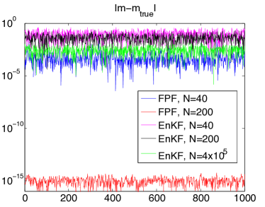
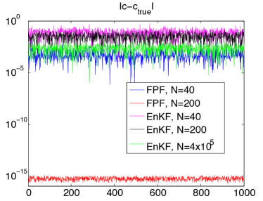
Fig. 1: OU process example. The relative error in the mean (left), and covariance (right) with respect to the true (Gaussian) filtering distribution for the Fokker-Planck filter MFEnKF-G2 (FPF) and the EnKF for several different cost levels $N$. Note the difference for EnKF is small owing to the $O(1/\sqrt{N})$ error, while the MFEnKF-G2 reaches numerical precision for $N=200$. EnKF for $N=4\times 10^{5}$ still performs worse than MFEnKF-G2 with $N=40$.

6.3 Nonlinear example

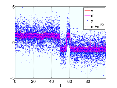
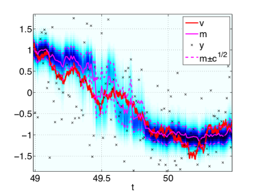
Fig. 2: The evolution (left) and close-up (right) of the filtering distribution for the continuous time Langevin process with a double-well external potential with discrete observations ($h=10^{-2},dt=10^{-4},\gamma=1$). The blue background shows the probability density, with darker corresponding to higher density. The symbols $v$, $m$, $y$, and $c$ correspond to the signal (or ”truth”), the mean, the observation, and the variance.

The Langevin diffusion process is considered here, in which $F(u)=au(1-u^{2})/(1+u^{2})$ in Eq. (12) with $a=10$. The dynamical noise level is $b=1/2$ and the observational noise variance is $\gamma^{2}=1$. The invariant distribution of the unconditioned state is again known, as described in the introduction to the section. Since $V$ has a double-well shape in this case, the invariant distribution is bimodal and paths of Equation (12) transition from one well to the other with a certain temporal probability. There is no analytical solution for the transient state, as there was in Section 6.2, and hence the transition kernel cannot be expressed in closed form.

Upon Euler-Marayuma discretization of time-step $dt$, we have

$$u_{k+1}=u_{k}+dtf(u_{k})+\sqrt{2bdt}\Delta_{k},$$ (54)

where $\Delta_{k}\sim N(0,1)$ are i.i.d. The discrete process $\{u_{k}\}$ does not have the same invariant distribution as $u(t)$ unless this is enforced with an accept-reject step [9]. Figure 2 shows the evolution of the filtering density in the background, with the truth ($v$), mean ($m$), standard deviation intervals ($m\pm c^{1/2}$), and observations ($y$) for a long time interval on the left, and a close-up interval on the right. In the case that the observation increment $h=ndt$ for $n>1$, we solve (54) for $n$ steps, and this approximates a draw from the kernel appearing in (1). Notice that this is a nonlinear and non-Gaussian state-space model, and we are now in the generalized framework.

A systematic series of numerical experiments is now performed with $dt=10^{-4}$ and $h=ndt$ where $n=5,20,100,$ and $1000$. The solution from algorithm full FPF with $N=1000$ is taken as the benchmark against which to evaluate the other methods, and we look at the relative RMSE over the time window $t\in[0,1000]$ with respect to the truth, and with respect to the mean and variance. The time window averaged over includes hundreds of transitions between wells, and so the results sufficiently incorporate transition behavior. The error of the full FPF with $N=200$ may be taken as the lower-bound error level of the benchmark.

The results are graphically presented in Figs. 6.3, 6.4, and 6.5. The term ”truth” in what follows refers to the signal realization $u$ which gave rise to the data, i.e. the realization $u$ which, together with the realization $\eta$, gave rise to the observed sequence $y$ with $y_{j}=Hu_{j}+\eta_{j}$. The following points summarize the plots:

• In the case of $n=5$ time-steps per observation, MFEnKF fails with $N=200$ degrees of freedom and requires $N=1000$ for convergence due to error in computation of the convolution . This is presumably because of the reduced relative resolution for the more narrow distribution in this case. For the other Fokker-Planck based algorithms the distribution is imperceptibly close for $N=200$ and $N=1000$ – this is a common criterion for determining convergence of numerical discretization.

• Only in the strongly nonlinear and non-Gaussian case, for $n=1000$, is there a notable difference between the methods in relative RMSE with respect to the truth. This is due presumably to the fact that in the other cases the RMSE between the truth and the mean of the filtering distribution is larger than the error between the mean and any of the approximate estimators. In this case, we observe the following from the close-up panel:

  • The mean of the full FPF gives the minimum RMSE.

  • The second place goes to MFEnKF-G1, which imposes Gaussianity only after the update. It is notable that in this strongly nonlinear and non-Gaussian case the RMSE is actually smaller if one performs the full nonlinear update and then imposes Gaussianity, rather than performing the linear update but retaining non-Gaussianity as in the MFEnKF.

  • The RMSE of MFEnKF-G2, which imposes Gaussianity of the forecast, is by far the greatest. The update to the mean and covariance here is the same as with the MFEnKF, but the resulting distribution does not retain any non-Gaussianity. It is therefore natural to expect worse performance.

  • The RMSE of EnKF is approximately equal to MFEnKF. One may therefore conclude that the linear error term is dominating. The RMSE of EnKF with a 200 member ensemble is close to but slightly greater than that with a 1000 member ensemble, and the latter is closer to MFEnKF as expected.

• For smaller numbers of time steps between observations, and hence a closer to linear and Gaussian kernel, the improvement of the MFEnK filters over the traditional EnKF with respect to mean and variance increases until for $n=5$ the RMSE of EnKF is almost an order of magnitude greater than that of the MFEnK filters.

• The statistics of the various MFEnK filters also converge to each other as $n$ decreases., indicating convergence to Gaussianity.

• The statistics of the Full FPF with 200 degrees of freedom indicates an accuracy level of the benchmark results, and this level also coincides with the MFEnK filters for $n=5$.

• The RMSE with respect to both mean and variance of MFEnKF-G1 is noticeably smaller than the other estimators for $n=1000$.

• For $n=5$ the RMSE of EnKF with $N=200$ is approximately twice that of EnKF with $N=1000$. This difference decreases as non-Gaussian error begins to play a role, until for $n=1000$ there is very little difference.

• With respect to tracking well-transitions in the strongly non-Gaussian regime ($h=1000dt=0.1$), it is worth emphasizing the observation that it is preferable to preserve the non-linearity of the update and impose Gaussianity, than to preserve some amount of non-Gaussianity and perform a linear update as in MFEnKF (see the $\square$ symbols associated to MFEnKF-G1). Of course imposing Gaussianity before the update results in a linear update anyway and performs the worst (see the $\times$ symbols associated to MFEnKF-G2). This can be related to the idea of implicit filtering [16, 59] and fixed-lag smoothing, and can build upon the observations related to tracking transitions from [42]. In the latter work, it was observed that a standard particle filter may fail to track due to lack of spread. This property is not shared by the deterministic approximation. In this regime the ranking of the methods in terms of signal tracking and in terms of approximation of the filtering distribution exactly coincide.

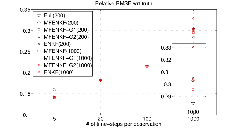
Fig. 3: Relative RMSE with respect to the truth of the various filters over various number of time-steps between observation updates with $dt=10^{-4}$.

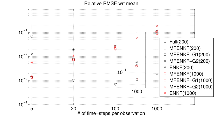
Fig. 4: Relative RMSE with respect to the mean of the various filters over various number of time-steps between observation updates with $dt=10^{-4}$.

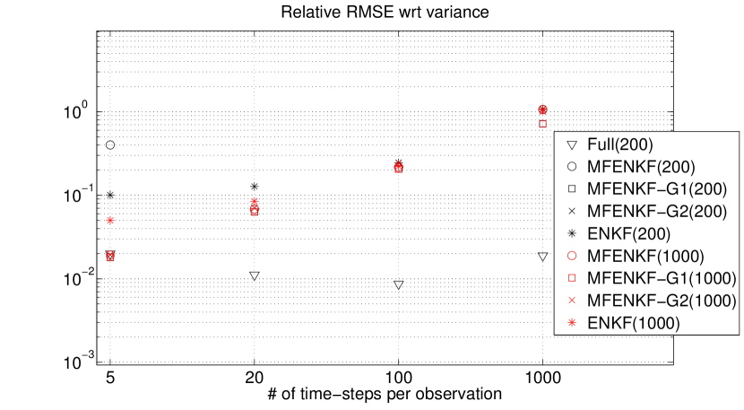
Fig. 5: Relative RMSE with respect to the variance of the various filters over various number of time-steps between observation updates with $dt=10^{-4}$.

7 Conclusion

A deterministic approach to mean-field ensemble Kalman filtering is considered for discrete-time observations of continuous stochastic processes. This approach is based on deterministic approximation of the density by numerical solution of the Fokker-Planck equation, and intermittent updates to the density based on quadrature rules. The scheme has a better rate of convergence in terms of degrees of freedom than corresponding Monte Carlo based methods for $d<2\kappa$, where $\kappa$ is the minimal order of the PDE solve and quadrature rule for $d=1$. In particular, the proposed DMFEnKF scheme converges faster to its linearly-biased limiting distribution than traditional EnKF methods, and the corresponding full filtering scheme converges faster to the true distribution than particle filtering methods. These results can be used to develop more effective filters. The use of more sophisticated discretization schemes should enable the extension of these methods to a much higher dimension $d$. Furthermore, it is well-known that very high-dimensional models may exhibit nonlinearity/instability/non-Gaussianity only on low-dimensional manifolds, so it is conceivable that deterministic solution techniques such as those developed here can be used on such manifold and combined with less expensive approximations on the complement. Hence it may be possible to extend such methods to real-world applications in the foreseeable future.

Acknowledgements The authors thank Jan Mandel for invaluable feedback in the initial revision, as well as the two referees whose careful and thorough review and suggestions have enormously improved the manuscript. Research reported in this publication was supported by the King Abdullah University of Science and Technology (KAUST). R. Tempone is a member of the KAUST SRI Center for Uncertainty Quantification. K.J.H.Law is a member of the Computer Science and Mathematics Division at Oak Ridge National Laboratory and was supported in part by KAUST SRI-UQ and in part by an ORNL LDRD Strategic Hire grant.

References

- [1] M Ades and PJ Van Leeuwen, An exploration of the equivalent weights particle filter, Quarterly Journal of the Royal Meteorological Society, 139 (2013), pp. 820–840.
- [2] A. Apte, C.K.R.T Jones, A.M. Stuart, and J. Voss, Data assimilation: mathematical and statistical perspectives, Int. J. Num. Meth. Fluids, 56 (2008), pp. 1033–1046.
- [3] Florian Augustin, A Gilg, M Paffrath, P Rentrop, and U Wever, Polynomial chaos for the approximation of uncertainties: chances and limits, European Journal of Applied Mathematics, 19 (2008), pp. 149–190.
- [4] A. Bain and D. Crisan, Fundamentals of Stochastic Filtering, Springer, 2009.
- [5] Feng Bao, Yanzhao Cao, Clayton Webster, and Guannan Zhang, A hybrid sparse-grid approach for nonlinear filtering problems based on adaptive-domain of the Zakai equation approximations, SIAM/ASA Journal on Uncertainty Quantification, 2 (2014), pp. 784–804.
- [6] P. Bickel, B. Li, and T. Bengtsson, Sharp failure rates for the bootstrap particle filter in high dimensions, IMS Collections: Pushing the Limits of Contemporary Statistics, 3 (2008), pp. 318–329.
- [7] D Blömker, K Law, AM Stuart, and KC Zygalakis, Accuracy and stability of the continuous-time 3DVAR filter for the Navier-Stokes equation, Nonlinearity, 26 (2012), p. 2193.
- [8] Adam Bobrowski, Functional analysis for probability and stochastic processes: an introduction, Cambridge University Press, 2005.
- [9] Nawaf Bou-Rabee and Eric Vanden-Eijnden, Pathwise accuracy and ergodicity of metropolized integrators for SDEs, Communications on Pure and Applied Mathematics, 63 (2010), pp. 655–696.
- [10] Michal Branicki and Andrew J Majda, Fundamental limitations of polynomial chaos for uncertainty quantification in systems with intermittent instabilities, Comm. Math. Sci, 11 (2012).
- [11] CEA Brett, KF Lam, KJH Law, DS McCormick, MR Scott, and AM Stuart, Accuracy and stability of filters for dissipative PDEs, Physica D: Nonlinear Phenomena, 245 (2012), pp. 34–45.
- [12] Hans-Joachim Bungartz and Michael Griebel, Sparse grids, Acta Numerica, 13 (2004), pp. 147–269.
- [13] Gerrit Burgers, Peter Jan van Leeuwen, and Geir Evensen, Analysis scheme in the ensemble Kalman filter, Monthly Weather Review, 126 (1998), pp. 1719–1724.
- [14] Olivier Cappé, Eric Moulines, and Tobias Rydén, Inference in hidden Markov models, Springer, 2005.
- [15] A.J. Chorin and P. Krause, Dimensional reduction for a Bayesian filter, Proc. Nat. Acad. Sci., 101 (2004), pp. 15013–15017.
- [16] Alexandre Chorin, Matthias Morzfeld, and Xuemin Tu, Implicit particle filters for data assimilation, Communications in Applied Mathematics and Computational Science, 5 (2010), pp. 221–240.
- [17] Pierre Del Moral and Alice Guionnet, On the stability of interacting processes with applications to filtering and genetic algorithms, in Annales de l’Institut Henri Poincaré (B) Probability and Statistics, vol. 37, Elsevier, 2001, pp. 155–194.
- [18] Roland L Dobrushin, Central limit theorem for nonstationary Markov chains. i,ii, Theory of Probability & Its Applications, 1 (1956), pp. 65–80.
- [19] Arnaud Doucet, Simon Godsill, and Christophe Andrieu, On sequential Monte Carlo sampling methods for Bayesian filtering, Statistics and computing, 10 (2000), pp. 197–208.
- [20] N. Doucet, A. de Frietas and N. Gordon, Sequential Monte Carlo in Practice, Springer-Verlag, 2001.
- [21] Tarek A El Moselhy and Youssef M Marzouk, Bayesian inference with optimal maps, Journal of Computational Physics, 231 (2012), pp. 7815–7850.
- [22] , Bayesian filtering with optimal maps, In preparation, (2014).
- [23] Oliver G Ernst, Björn Sprungk, and Hans-Jörg Starkloff, Bayesian inverse problems and Kalman filters, in Extraction of Quantifiable Information from Complex Systems, Springer, 2014, pp. 133–159.
- [24] L.C. Evans, Partial Differential Equations, AMS, Providence, Rhode Island, 1998.
- [25] Lawrence C Evans, An introduction to stochastic differential equations, vol. 82, American Mathematical Soc., 2012.
- [26] Geir Evensen, Sequential data assimilation with a nonlinear quasi-geostrophic model using monte carlo methods to forecast error statistics, Journal of Geophysical Research: Oceans (1978–2012), 99 (1994), pp. 10143–10162.
- [27] Gregory L Eyink, Juan M Restrepo, and Francis J Alexander, A mean field approximation in data assimilation for nonlinear dynamics, Physica D: Nonlinear Phenomena, 195 (2004), pp. 347–368.
- [28] K. Hayden, E. Olson, and E.S. Titi, Discrete data assimilation in the Lorenz and 2d Navier-Stokes equations, Physica D: Nonlinear Phenomena, (2011).
- [29] Ibrahim Hoteit, Xiaodong Luo, and Dinh-Tuan Pham, Particle Kalman filtering: A nonlinear Bayesian framework for ensemble Kalman filters, arXiv:1108.0168, (2011).
- [30] A.H. Jazwinski, Stochastic processes and filtering theory, vol. 63, Academic Pr, 1970.
- [31] J.P. Kaipio and E. Somersalo, Statistical and computational inverse problems, Springer Science+ Business Media, Inc., 2005.
- [32] Rudolph Emil Kalman et al., A new approach to linear filtering and prediction problems, Journal of basic Engineering, 82 (1960), pp. 35–45.
- [33] E. Kalnay, Atmospheric Modeling, Data Assimilation and Predictability, Cambridge, 2003.
- [34] D.T.B. Kelly, K.J.H. Law, and A.M. Stuart, Well-posedness and accuracy of the ensemble Kalman filter in discrete and continuous time. Submitted.
- [35] Evan Kwiatkowski and Jan Mandel, Convergence of the square root ensemble Kalman filter in the large ensemble limit, SIAM/ASA Journal on Uncertainty Quantification, 3 (2015), pp. 1–17.
- [36] Pierre Simon Laplace, Memoir on the probability of the causes of events, Statistical Science, (1986), pp. 364–378.
- [37] KJH Law and AM Stuart, Evaluating data assimilation algorithms, Monthly Weather Review, 140 (2012), pp. 3757–3782.
- [38] Kody J H Law, Andrew M Stuart, and Konstantinos C Zygalakis, Data Assimilation: A Mathematical Introduction, Springer Texts in Applied Mathematics, 2015.
- [39] François Le Gland, Valérie Monbet, Vu-Duc Tran, et al., Large sample asymptotics for the ensemble Kalman filter, The Oxford Handbook of Nonlinear Filtering, (2011), pp. 598–631.
- [40] Jia Li and Dongbin Xiu, A generalized polynomial chaos based ensemble Kalman filter with high accuracy, Journal of computational physics, 228 (2009), pp. 5454–5469.
- [41] David G Luenberger, Optimization by vector space methods, John Wiley & Sons, 1969.
- [42] Jan Mandel and Jonathan D Beezley, An ensemble Kalman-particle predictor-corrector filter for non-Gaussian data assimilation, in Computational Science–ICCS 2009, Springer, 2009, pp. 470–478.
- [43] Jan Mandel, Loren Cobb, and Jonathan D Beezley, On the convergence of the ensemble Kalman filter, Applications of Mathematics, 56 (2011), pp. 533–541.
- [44] P. A. Markowich and C. Villani, On the trend to equilibrium for the Fokker-Planck equation: an interplay between physics and functional analysis, Mat. Contemp., 19 (2000), pp. 1–29.
- [45] Jonathan C Mattingly, Andrew M Stuart, and Desmond J Higham, Ergodicity for sdes and approximations: locally lipschitz vector fields and degenerate noise, Stochastic processes and their applications, 101 (2002), pp. 185–232.
- [46] B. Oksendal, Stochastic differential equations, Universitext, Springer, sixth ed., 2003. An introduction with applications.
- [47] Oliver Pajonk, Stochastic Spectral Methods for Linear Bayesian Inference, PhD thesis.
- [48] Oliver Pajonk, Bojana V Rosić, Alexander Litvinenko, and Hermann G Matthies, A deterministic filter for non-Gaussian Bayesian estimation applications to dynamical system estimation with noisy measurements, Physica D: Nonlinear Phenomena, 241 (2012), pp. 775–788.
- [49] Oliver Pajonk, Bojana V Rosić, and Hermann G Matthies, Sampling-free linear Bayesian updating of model state and parameters using a square root approach, Computers & Geosciences, 55 (2013), pp. 70–83.
- [50] Patrick Rebeschini and Ramon van Handel, Can local particle filters beat the curse of dimensionality?, arXiv:1301.6585, (2013).
- [51] Sebastian Reich, A Gaussian-mixture ensemble transform filter, Quarterly Journal of the Royal Meteorological Society, 138 (2012), pp. 222–233.
- [52] H. Risken, The Fokker-Planck equation, vol. 18 of Springer Series in Synergetics, Springer-Verlag, Berlin, 1989.
- [53] H Salman, A hybrid grid/particle filter for Lagrangian data assimilation. i: Formulating the passive scalar approximation, Quarterly Journal of the Royal Meteorological Society, 134 (2008), pp. 1539–1550.
- [54] Naratip Santitissadeekorn and Chris Jones, Two-state filtering for joint state-parameter estimation, arXiv:1403.5989, (2014).
- [55] Themistoklis P Sapsis and Andrew J Majda, Blended reduced subspace algorithms for uncertainty quantification of quadratic systems with a stable mean state, Physica D: Nonlinear Phenomena, (2013).
- [56] Antti Solonen, Heikki Haario, Janne Hakkarainen, Harri Auvinen, Idrissa Amour, and Tuomo Kauranne, Variational ensemble Kalman filtering using limited memory BFGS, Electronic Transactions on Numerical Analysis, 39 (2012), pp. 271–285.
- [57] A.M. Stuart, Inverse problems: a Bayesian approach, Acta Numerica, 19 (2010), pp. 451–559.
- [58] F Uboldi, A Trevisan, A Carrassi, et al., Developing a dynamically based assimilation method for targeted and standard observations, Nonlinear Processes in Geophysics, 12 (2005), pp. 149–156.
- [59] Eric Vanden-Eijnden and Jonathan Weare, Data assimilation in the low noise, accurate observation regime with application to the Kuroshio current, Monthly Weather Review, 141 (2012), p. 1.