A random shock model with mixed effect, including competing soft and sudden failures, and dependence

Abstract

A system is considered, which is subject to external and possibly fatal shocks, with dependence between the fatality of a shock and the system age. Apart from these shocks, the system suffers from competing soft and sudden failures, where soft failures refer to the reaching of a given threshold for the degradation level, and sudden failures to accidental failures, characterized by a failure rate. A non-fatal shock increases both degradation level and failure rate of a random amount, with possible dependence between the two increments. The system reliability is calculated by four different methods. Conditions under which the system lifetime is New Better than Used are proposed. The influence of various parameters of the shocks environment on the system lifetime is studied.

Keywords: Reliability; Bivariate non homogeneous compound Poisson process; Hazard rate process; Poisson random measure; Stochastic order; Ageing properties; Two-component series system.

AMS MSC: 60K10 & 60G51

1 Introduction

This paper is devoted to the survival analysis of a system subject to competing failure modes within an external stressing environment. The external environment is assumed to stress the system at random and isolated times according to a random shock model. Such a model can represent external demands e.g., which put some stress on the system at their arrivals. Shock models have been the subject of an extensive literature. Following Mallor and Santos (2003a), shock models may be classified into different categories, according to whether arrival times and shock magnitudes are correlated (Mallor and Omey, 2001; Mallor and Santos, 2003b), or independent (Cha and Finkelstein, 2009), and according to the assumption put on the shocks arrival process: homogeneous or non-homogeneous Poisson process (A-Hameed and Proschan, 1973; Cha and Finkelstein, 2009; Cha and Mi, 2007, 2011; Esary et al., 1973; Qian et al., 1999), renewal process (Skoulakis, 2000) or non-stationary pure birth process (A-Hameed and Proschan, 1975). According to the influence of shocks on the system, shock models may be further classified into three types: extreme shock models (a shock can cause the system immediate failure, see Gut and Hüsler 1999), cumulative shock models (a shock increases some intrinsic characteristic of the system such as its deterioration, failure rate, age, number of already endured shocks, …, see Cha and Mi 2007; Qian et al. 1999) and mixed shock models (a shock can either cause the system immediate failure or increase some intrinsic characteristic, see Cha and Mi 2011; Gut 2001). More references can be found in Finkelstein and Cha (2013); Mallor and Santos (2003a); Nakagawa (2007); Singpurwalla (1995).

In this paper, a shock model with mixed effects is considered, where the occurrence of shocks is classically modelled through a non-homogeneous Poisson process and where each shock may result in the system immediate failure through a Bernoulli trial, independent of the system intrinsic behaviour. Apart from shocks, the system suffers from competing soft and sudden failures, where soft failures refer to the reaching of some given threshold for the degradation level, and sudden failures to accidental failures, characterized by a failure rate. A possible representation corresponds to a two-component series system, where the first component is subject to soft failures and the second one to sudden failure. The system may hence fail through three different competing modes: traumatic failure due to a fatal shock; soft failure; sudden failure. Each non fatal shock induces some increase of both deterioration level and failure, with possible dependence in-between.

In the oldest literature, most models considered one single possible type of failures for the system: e.g. soft failures in Marshall and Shaked (1979) or traumatic failures due to shocks in Savits (1988), both in the multivariate setting. More recently, different models have been developed, which consider two different types of failures. For instance, competition between soft and sudden failures is studied in Zhu et al. (2010). Several application cases are proposed in the paper (see also references therein). An industrial example is also provided in Wang and Gao (2014), which studies the reliability of an aircraft engine. Note that Zhu et al. (2010) assumes soft and sudden failures to be independent whereas the stressing environment of the present paper makes them dependent. Competition between soft failures and occurrence of a traumatic event are considered in Degradation-Threshold-Shock models (DTS-models, denomination of Lehmann 2006) which have been proposed by Lemoine and Wenocur (1985) and further studied by Lehmann (2006, 2009). A case study is provided in Hao et al. (2013) for the analysis of fatigue crack growth, where the effects of shocks on the degradation are put into evidence. Note that, contrary to the present paper, DTS-models consider some possible influence of the deterioration level of the system on the shocks arrival rate. However, the first shock of a DTS-model is always fatal to the system (leading to a single shock possibly endured by the system), whereas successive non fatal shocks are here envisioned. We could not find any paper which takes into account three competing failure modes, as in the present paper. However, based on the case studies from the previous literature, one can think that our model can reflect lots of systems subject to competing soft and hard failures, within a stressing environment. For instance, one can think of an aerial cabin hooked to a cable: the supporting cable is deteriorating due to corrosion and fatigue; the linking pulley is subject to sudden failures (and maybe also to deterioration); both cable and pulley endure shocks at each cabin travel, which increase jointly their respective deterioration level and failure rate.

The present paper consider several kinds of dependence between the three competing failure modes: at each non fatal shock, the increase of deterioration and failure rate is simultaneous. This induces a first type of dependence between soft and sudden failures. Each shock may induce a failure, either because the shock is fatal, or because the deterioration is suddenly increased beyond the threshold level. This induces a second type of dependence between soft and traumatic failures, which may be simultaneous. Also, some possible dependence is envisioned between the increments of failure rate and of deterioration at each non fatal shock. This induces a third type of dependence between soft and sudden failures. Finally, following Cha and Finkelstein (2009); Cha and Mi (2011), the probability for a shock to be fatal depends on the shock arrival time, which induces a last type of dependence. Up to our knowledge, all these kinds of dependence have not been yet considered altogether and, as will be seen all along the text, this model enlarges several ones from the previous literature.

The paper is organized as follows: the model is specified in Section 2. The system reliability is computed through different methods in Section 3. Sufficient conditions are provided in Section 4 for the system lifetime to be New Better than Used. The influence of various parameters of the shock environment on the lifetime is studied in Section 5. Numerical experiments are proposed in Section 6 and concluding remarks end the paper in Section 7.

2 The model

To make the model clear, a two-component series system is considered, where the first component is subject to sudden failure and the second one to soft failure. This two-unit system is just a representation for the competing soft and sudden failure modes, with no restriction. In the ideal condition (for example in a laboratory environment), the lifetime of the first component is characterized by its intrinsic hazard rate $h(t)$, $t\geq 0$ while the second one is subject to some accumulative deterioration modeled by an increasing stochastic process $(G_{t})_{t\geq 0}$ (e.g. a gamma process). The second component fails once its deterioration level exceeds a failure threshold $L$. The lifetimes of the two components are made dependent by their common stressing environment. This environment is modelled by a random shock process, where the shocks arrive according to a non-homogeneous Poisson process $(N_{t})_{t\geq 0}$ with intensity $d\Lambda(t)=\lambda(t)dt$ (or cumulated intensity $\Lambda(t)$). To avoid useless technical details, we assume that $\Lambda\left(t\right)>0$ for all $t>0$. More generally, one might consider that $\Lambda\left(t\right)>0$ only for $t$ greater than some $t_{0}>0$, which would mean that the shocks would arrive only after time $t_{0}$. The points of the Poisson process are denoted by $T_{1}$, …, $T_{n}$, … with $T_{0}=0<T_{1}<\ldots<T_{n}<\ldots$ almost surely. A shock at time $t$ may cause the system immediate failure (fatal shock) with probability $p(t)\in[0,1]$, which depends on the age $t$ of the system at the shock arrival. A shock at time $t$ is non fatal with probability $q\left(t\right)=1-p\left(t\right)$. A non fatal shock at time $T_{i}$ increases the deterioration of both components in a different way:

• for the first component, its hazard rate is increased of a non negative random amount $V_{i}^{(1)}$,

• for the second one, its accumulated deterioration is increased of a non negative random amount $V_{i}^{(2)}$.

The random vectors $V_{i}=\left(V_{i}^{(1)},V_{i}^{(2)}\right)$, $i=1$, $2$, … are assumed to be independent and identically distributed (i.i.d.) with common distribution $\mu(dv_{1},dv_{2})$, and independent of the shocks arrival times $(T_{n})_{n\geq 1}$ (and hence independent of the Poisson process $(N_{t})_{t\geq 0}$). At each shock, the increments $V_{i}^{(1)}$ and $V_{i}^{(2)}$ are possibly dependent. When subscript $i$ is unnecessary, we drop it and set $V=\left(V^{\left(1\right)},V^{\left(2\right)}\right)$ to be a generic copy of $V_{i}=\left(V_{i}^{(1)},V_{i}^{(2)}\right)$. For $j=1,2$, the distribution of $V^{\left(j\right)}$ is denoted by $\mu_{j}(dv_{j})$.

We set $\left(A_{t}\right)_{t\geq 0}$ to be the bivariate compound Poisson process defined by

$$A_{t}=\left(\sum_{k=1}^{N_{t}}V_{k}^{(1)},\sum_{k=1}^{N_{t}}V_{k}^{(2)}\right)=\left(A_{t}^{\left(1\right)},A_{t}^{\left(2\right)}\right)$$ (1)

with

$$A_{t}^{(1)} ={\sum_{k=1}^{N_{t}}V_{k}^{(1)},}$$

$$A_{t}^{(2)} ={\sum_{k=1}^{N_{t}}V_{k}^{(2)},}$$

where $\sum_{k=1}^{0}\cdots=0$.

The processes $(A_{t})_{t\geq 0}$ and $(G_{t})_{t\geq 0}$ are assumed to be independent.

Provided that the system is functioning up to time $t$, the random variables $A_{t}^{(1)}$ and $A_{t}^{(2)}$ stand for the cumulated increments on $\left[0,t\right]$ of the failure rate of the first component and of the deterioration of the second component due to the external environment, respectively. Setting $\mathcal{F}_{t}=\sigma\left(A_{s},s\leq t\right)$ to be the $\sigma-$field generated by $\left(A_{s}\right)_{s\leq t}$ and provided that the system is still up at time $t$, the conditional hazard rate of the first component given $\mathcal{F}_{t}$ is

$$X_{t}^{(1)}=h(t)+A_{t}^{(1)}$$

and the conditional deterioration of the second component given $\mathcal{F}_{t}$ is

$$X_{t}^{(2)}=G_{t}+A_{t}^{(2)}.$$

To make it clearer, we introduce $\tau_{i}$, $i=1,2$ to be the lifetime of the $i^{th}$ component under the external environment, without taking into account the possibility of fatal shocks for the system. To simplify the writing, we denote by $\mathbb{P}\left(B|\mathcal{F}_{t}\right)$ the conditional expectation $\mathbb{E}\left(\mathbf{1}_{B}|\mathcal{F}_{t}\right)$ for any measurable set $B$, where $\mathbf{1}_{B}$ stands for the indicator function ($\mathbf{1}_{B}\left(\omega\right)=1$ if $\omega\in B$, 0 elsewhere). We then have:

$$\mathbb{P}\left(\tau_{1}>t|\mathcal{F}_{t}\right) =e^{-\int_{0}^{t}X_{s}^{(1)}~{}ds}=e^{-H\left(t\right)}e^{-\int_{0}^{t}A_{s}^{(1)}~{}ds},$$ (2)

$$\mathbb{P}\left(\tau_{2}>t|\mathcal{F}_{t}\right) =\mathbb{P}\left(X_{t}^{(2)}\leq L|\mathcal{F}_{t}\right)=\mathbb{P}\left(G_{t}\leq L-A_{t}^{(2)}|\mathcal{F}_{t}\right)=F_{G_{t}}\left(L-A_{t}^{\left(2\right)}\right)$$ (3)

where

$$H\left(t\right)=\int_{0}^{t}h(s)~{}ds$$ (4)

is the cumulated intrinsic failure rate of the first component and where $F_{G_{t}}$ stands for the cumulative distribution function (c.d.f.) of $G_{t}$. (Recall that $G_{t}$ is independent of $\mathcal{F}_{t}$).

We now let $\tau_{3}$ to be the time to the first fatal shock for the system with

$$\tau_{3}=\inf\left(n\geq 1:\text{ the shock at time }T_{n}\text{ is fatal}\right)$$

and we assume that the Bernoulli trials (fatal shocks or not) which happen at each shock arrival are independent one with each other, and that they depend on $\mathcal{F}_{t}$ only through the $q\left(T_{n}\right)$’s, that is:

$$\mathbb{P}\left(\tau_{3}>t|\mathcal{F}_{t}\right)=\prod_{i=1}^{\infty}q\left(T_{i}\right)\mathbf{1}_{\left[0,t\right]}\left(T_{i}\right)=\prod_{i=1}^{N_{t}}q\left(T_{i}\right)$$ (5)

where $\prod_{i=1}^{0}\cdots=1$.

The system failure is induced either by a fatal shock or by a component failure (soft or sudden failure), whatever arrives first. The lifetime of the system hence is

$$\tau=\min\left(\tau_{1},\tau_{2},\tau_{3}\right).$$ (6)

We finally make the additional assumption that $\tau_{1}$, $\tau_{2}$ and $\tau_{3}$ are conditionally independent given $\mathcal{F}_{t}:$

$$\mathbb{P}\left(\tau_{1}>t,\tau_{2}>t,\tau_{3}>t|\mathcal{F}_{t}\right)$$

$$=\mathbb{P}\left(\tau_{1}>t|\mathcal{F}_{t}\right)\mathbb{P}\left(\tau_{2}>t|\mathcal{F}_{t}\right)\mathbb{P}\left(\tau_{3}>t|\mathcal{F}_{t}\right).$$

To sum up, the whole model is specified by:

• $\left(V^{\left(1\right)},V^{\left(2\right)}\right):$ the (generic) random increments in failure rate (first component, $V^{\left(1\right)}$) and deterioration (second component, $V^{\left(2\right)}$),

• $\lambda\left(x\right)dx:$ the intensity of the non-homogeneous Poisson process,

• $h\left(x\right):$ the intrinsic failure rate of the first component (sudden failure),

• $(G_{t})_{t\geq 0}:$ the intrinsic deterioration of the second component (soft failure),

• $p\left(t\right):$ the probability for a shock at time $t$ to be fatal at the system level,

(plus some independence assumptions).

By taking special cases for these five ingredients, we can see that our model extents some well-known models from the literature.

For instance, taking $p\left(t\right)=0$ (no fatal shocks), $V^{\left(1\right)}=$ constant, $V^{\left(2\right)}=0$ and $G_{t}=0$ all $t\geq 0$ (no second component), one gets the ”stochastic failure model in random environment” from Cha and Mi (2007).

Taking $V^{\left(2\right)}=0$ and $G_{t}=0$ all $t\geq 0$ (one single component), one gets the ”stochastic survival model for a system under randomly variable environment” from Cha and Mi (2011).

Taking $G_{t}=0$ all $t\geq 0$, $V^{\left(1\right)}=V^{\left(2\right)}=0$, the model resumes to a classical extreme shock model (one single component), where system failures are only due to shocks arriving according to a non-homogeneous Poisson process, with probability $p\left(t\right)$ for a shock to be fatal (and $q\left(t\right)$ to be harmless). This model is interpreted as the Brown-Proschan model by Cha and Finkelstein (2009); see also Brown and Proschan (1983) where various properties of the model are explored.

Taking $p\left(t\right)=0$ (no fatal shocks), $V^{\left(1\right)}=h\left(t\right)=0$ (one single component), $\lambda\left(x\right)=\lambda$ (homogeneous Poisson process), $G_{t}=0$ all $t\geq 0$ (no intrinsic deterioration for the second - and single - component), one gets the ”cumulative damage threshold model” from (Esary et al., 1973, Section 4, case of i.i.d. damage increments).

Taking $p\left(t\right)=p$ (constant), $V^{\left(1\right)}=h\left(t\right)=0$ (one single component), $G_{t}=0$ all $t\geq 0$, one gets the ”cumulative damage model with two kinds of shocks” from (Qian et al., 1999, case of i.i.d. damage increments).

Taking $V^{\left(1\right)}=h=0$, $V^{\left(2\right)}$ exponentially distributed, $G_{t}=t$, all $t\geq 0$, one gets the model from Subsection 3.b in Cha and Finkelstein (2009).

All these models are summed up in Table 1. Note that we do not pretend at any exhaustibility and our model will include lots of other previous models which are not provided here.

Table 1: A few particular models from the literature

Brown-Proschan model from (Brown and Proschan, 1983)	$h=V^{\left(1\right)}=V^{\left(2\right)}=0$,
	$G_{t}=0$, $\forall t\geq 0$
Deterministic boundary in (Cha and Finkelstein, 2009)	$V^{\left(1\right)}=h=0$, $G_{t}=t$
	$V^{\left(2\right)}$ exponentially distributed
Cha and Mi (2007)	$q=1$, $V^{(1)}$ is a constant,
	$V^{\left(2\right)}=0$, $G_{t}=0$, $\forall t\geq 0$
Cha and Mi (2011)	$V^{\left(2\right)}=0$, $G_{t}=0$, $\forall t\geq 0$
Cumulative damage threshold models	$q=1$, $V^{\left(2\right)}=0$, $\lambda$ is a constant
in Section 4 of (Esary et al., 1973)	$h=0$, $G_{t}=0$, $\forall t\geq 0$
Qian et al. (1999)	$q$ is a constant, $h=V^{\left(1\right)}=0$,
	$G_{t}=0$, $\forall t\geq 0$

3 Calculation of the system reliability

The objective of this section is to calculate the reliability $R_{L}(t)$ of the system at time $t$, with

$$R_{L}(t)=\mathbb{P}(\tau>t),\text{ all }t\geq 0,$$

where we recall that the system lifetime $\tau$ is defined by $\left(\ref{tau}\right)$.

A first way to compute $R_{L}(t)$ is to use classical Monte-Carlo simulations and to simulate a large number of independent histories for the system up to time $t$ (Method 1). This method will serve as a comparison tool in the numerical experimentations in Section 6. This method requires the simulation of a random variable with conditional hazard rate $h(t)+{\sum_{k=1}^{N_{t}}V_{k}^{(1)}}$ (see Algorithm 12 in Section 6 for details) and may imply long computational times for the system reliability. We provide below a few alternate methods which may be quicker and also easier to implement.

Proposition 1 (Method 2)

The reliability is given by

$$R_{L}(t)=\mathbb{P}(\tau>t)=e^{-H(t)}\phi_{t}(L),$$ (7)

where $H\left(t\right)$ is provided by $\left(\ref{H}\right)$ and where

$$\phi_{t}(L) =\mathbb{E}\left(F_{G_{t}}\left(L-A_{t}^{\left(2\right)}\right)e^{-\int_{0}^{t}A_{s}^{(1)}~{}ds}\prod_{i=1}^{N_{t}}q\left(T_{i}\right)\right)$$ (8)

$$=\mathbb{E}\left(F_{G_{t}}\left(L-\sum_{i=1}^{N_{t}}V_{i}^{(2)}\right)e^{-\sum_{i=1}^{N_{t}}V_{i}^{(1)}(t-T_{i})}\prod_{i=1}^{N_{t}}q(T_{i})\right)$$ (9)

Proof. Due to the conditional independence of $\tau_{1}$, $\tau_{2}$ and $\tau_{3}$ given $\mathcal{F}_{t}$, we have:

$$R_{L}(t) =\mathbb{P}(\tau_{1}>t,\tau_{2}>t,\tau_{3}>t)$$

$$=\mathbb{E}\left(\mathbb{P}\left(\tau_{1}>t,\tau_{2}>t,\tau_{3}>t|\mathcal{F}_{t}\right)\right)$$

$$=\mathbb{E}\left(\mathbb{P}\left(\tau_{1}>t|\mathcal{F}_{t}\right)\mathbb{P}\left(\tau_{2}>t|\mathcal{F}_{t}\right)\mathbb{P}\left(\tau_{3}>t|\mathcal{F}_{t}\right)\right).$$

Using $\left(\ref{tau1},\ref{tau2},\ref{tau3}\right)$, we get:

$$R_{L}(t)=\mathbb{E}\left(e^{-H\left(t\right)}e^{-\int_{0}^{t}A_{s}^{(1)}~{}ds}~{}F_{G_{t}}\left(L-A_{t}^{\left(2\right)}\right)~{}\prod_{i=1}^{N_{t}}q\left(T_{i}\right)\right),$$

which provides $\left(\ref{eq_phi1}\right)$ and next $\left(\ref{eq_phi2}\right)$, due to $\left(\ref{At_i}\right)$ and

$$\int_{0}^{t}A_{s}^{(1)}~{}ds =\int_{0}^{t}\sum_{i=1}^{+\infty}V_{i}^{(1)}\mathbf{1}_{\left\{T_{i}\leq s\right\}}~{}ds=\sum_{i=1}^{+\infty}V_{i}^{(1)}\int_{0}^{t}\mathbf{1}_{\left\{T_{i}\leq s\right\}}~{}ds$$

$$=\sum_{i=1}^{+\infty}V_{i}^{(1)}(t-T_{i})\mathbf{1}_{\left\{T_{i}\leq t\right\}}=\sum_{i=1}^{N_{t}}V_{i}^{(1)}(t-T_{i}).$$ (10)

 

Based on the previous result, the only point to get the reliability $R_{L}(t)$ is to compute $\phi_{t}(L)$. The remaining of the section is hence devoted to the computation of $\phi_{t}(L)$. Starting from $\left(\ref{eq_phi1}\right)$ (or $\left(\ref{eq_phi2}\right)$), a possibility is to compute $\phi_{t}(L)$ through Monte-Carlo simulations of $\left(N_{t}\right)_{t\geq 0}$ and $\left(A_{t}\right)_{t\geq 0}$, which is simpler and quicker than simulating trajectories of the system according to the initial model. This method is called Method 2 in Section 6.

Following A-Hameed and Proschan (1973) and Esary et al. (1973), one may also use a series expansion of $\phi_{t}(L)$, as provided by the following proposition.

Proposition 2 (Method 3, general case)

$$\phi_{t}(L)=e^{-\Lambda(t)}\sum_{n=0}^{\infty}P_{n}\left(t,L\right)\frac{(\Lambda(t))^{n}}{n!}$$ (11)

where

$$P_{n}\left(t,L\right)=\mathbb{E}\left(F_{G_{t}}\left(L-\sum_{i=1}^{n}V_{i}^{(2)}\right)\prod_{i=1}^{n}\left(q(Z_{i})e^{-(t-Z_{i})V_{i}^{(1)}}\right)\right)$$ (12)

and $(Z_{i})_{i\geq 1}$ are i.i.d. random variables with probability density function (p.d.f.) $\frac{\lambda(x)}{\Lambda(t)}1_{[0,t]}(x)$ and independent of $\left(V_{i}\right)_{i\geq 1}$.

Proof. Conditioning on the Poisson process $\left(N_{t}\right)_{t\geq 0}$, we have:

$$\phi_{t}(L)=\mathbb{E}\left(f\left(N_{t}\right)\right)=\sum_{n=0}^{+\infty}f\left(n\right)\frac{(\Lambda(t))^{n}}{n!}e^{-\Lambda(t)}$$

with

$$f\left(n\right)=\mathbb{E}\left(F_{G_{t}}\left(L-\sum_{i=1}^{N_{t}}V_{i}^{(2)}\right)\prod_{i=1}^{N_{t}}q(T_{i})e^{-\sum_{i=1}^{N_{t}}(t-T_{i})V_{i}^{(1)}}|N_{t}=n\right).$$

Now, given that $N_{t}=n$, the conditional joint distribution of $(T_{1},\ldots T_{n})$ is the same as the joint distribution of the order statistics $(Z_{\left(1\right)},\ldots,Z_{\left(n\right)})$ of $n$ i.i.d. random variables $Z_{1},\ldots,Z_{n}$ with p.d.f. $\frac{\lambda(x)}{\Lambda(t)}1_{[0,t]}(x)$ (see Cocozza-Thivent 1998 e.g.). Using the fact that $V_{i}=\left(V_{i}^{\left(1\right)},V_{i}^{\left(2\right)}\right)$ is independent of $\left(N_{t}\right)_{t\geq 0}$, we get:

$$f\left(n\right)=\mathbb{E}\left(F_{G_{t}}\left(L-\sum_{i=1}^{n}V_{i}^{(2)}\right)\prod_{i=1}^{n}q(Z_{\left(i\right)})e^{-\sum_{i=1}^{n}(t-Z_{\left(i\right)})V_{i}^{(1)}}\right).$$

Noting that the expression within the expectation is invariant through permutation of the $Z_{i}$’s, we derive that:

$$f\left(n\right)=\mathbb{E}\left(F_{G_{t}}\left(L-\sum_{i=1}^{n}V_{i}^{(2)}\right)\prod_{i=1}^{n}q(Z_{i})e^{-\sum_{i=1}^{n}(t-Z_{i})V_{i}^{(1)}}\right),$$

which provides the result.   

Remark 3

Based on the previous result, one can see that our model is equivalent to a classical shock model, where the shocks arrive according to a non-homogeneous Poisson process with intensity $d\Lambda(x)$ and with conditional probability of survival at time $t$ equal to $P_{n}\left(t,L\right)$, given that there has been $n$ shocks up to time $t$.

Corollary 4 (Method 3, independent case)

In the special case where $V^{\left(1\right)}$ and $V^{(2)}$ are independent, we get:

$$\phi_{t}(L)=e^{-\Lambda(t)}\sum_{n=0}^{\infty}Q_{n}\left(t,L\right)\frac{(a(t))^{n}}{n!}$$ (13)

with

$$Q_{n}\left(t,L\right)=\mathbb{E}\left(F_{G_{t}}\left(L-\sum_{i=1}^{n}V_{i}^{(2)}\right)\right)$$ (14)

and

$$a(t)=\left(\tilde{\mu}_{1}\ast(q\lambda)\right)(t)=\color[rgb]{0,0,0}\int_{0}^{t}\tilde{\mu}_{1}(z)(q\lambda)(t-z)~{}dz,$$ (15)

where $\ast$ stands for the convolution operator, $(q\lambda)(x)=q(x)\lambda(x)$, all $x\geq 0$, and $\tilde{\mu}_{1}$ stands for the Laplace transform of the distribution $\mu_{1}$ of $V^{\left(1\right)}$, with

$$\tilde{\mu}_{1}\left(s\right)=\int_{0}^{+\infty}e^{-xs}\mu_{1}\left(dx\right)\text{, all }s\geq 0.$$

Proof. Starting from $\left(\ref{PnGen}\right)$ and using the independence of all $V_{i}^{\left(1\right)}$’s, $V_{i}^{\left(2\right)}$’s and $Z_{i}$’s, and the identical distributions of all $V_{i}^{\left(1\right)}$’s and of all $Z_{i}$’s, we get:

$$P_{n}\left(t,L\right)=\mathbb{E}\left(F_{G_{t}}\left(L-\sum_{i=1}^{n}V_{i}^{(2)}\right)\right)\left(\mathbb{E}\left(q(Z_{1})e^{-(t-Z_{1})V^{(1)}}\right)\right)^{n}$$ (16)

with

$$\mathbb{E}\left(q(Z_{1})e^{-(t-Z_{1})V^{(1)}}\right) =\frac{1}{\Lambda(t)}\int_{0}^{t}\lambda(z)q\left(z\right)\mathbb{E}\left(e^{-(t-z)V^{(1)}}\right)dz$$

$$=\frac{1}{\Lambda(t)}\int_{0}^{t}\left(\lambda q\right)(z)\tilde{\mu}_{1}\left(t-z\right)dz=\frac{a\left(t\right)}{\Lambda\left(t\right)}.$$

Substituting this expression into Eq. $\left(\ref{Pn2}\right)$ and next into Eq. $\left(\ref{PnGen}\right)$ provides the result.   

Example 5

Let $V^{(2)}$ be an exponentially distributed with mean $1/\theta$ and $V^{\left(1\right)}$ an independent random variable. In that case, $\sum_{i=1}^{n}{V}_{i}^{(2)}$ is Gamma distributed with parameter $\left(n,\theta\right)$. This provides

$$Q_{n}\left(t,L\right)=\int_{0}^{L}F_{G_{t}}(L-x)\frac{\theta^{n}x^{n-1}}{(n-1)!}e^{-\theta x}~{}dx,\,\text{all }n\geq 1.$$

Using $Q_{0}\left(t,L\right)=F_{G_{t}}\left(L\right)$ and Eq. $\left(\ref{eq1}\right)$, we get:

$$R_{L}(t)=e^{-H(t)-\Lambda(t)}\left(F_{G_{t}}(L)+\sum_{n=1}^{\infty}\frac{(a(t))^{n}}{n!}\int_{0}^{L}F_{G_{t}}(L-x)\frac{\theta^{n}x^{n-1}}{(n-1)!}e^{-\theta x}~{}dx\right).$$

Taking $G_{t}=t$ for all $t\geq 0$, $V^{\left(1\right)}=0$ and $h\left(t\right)=0$ as a special case, we get

$$F_{G_{t}}\left(L\right) =\mathbf{1}_{\left\{t\leq L\right\}},$$

$$a(t) =\int_{0}^{t}\left(q\lambda\right)\left(s\right)ds$$

and, for $t\leq L:$

$$R_{L}(t) =e^{-\Lambda(t)}\left(1+\sum_{n=1}^{\infty}\frac{(\int_{0}^{t}\left(q\lambda\right)\left(s\right)ds)^{n}}{n!}\int_{0}^{L-t}\frac{\theta^{n}x^{n-1}}{(n-1)!}e^{-\theta x}~{}dx\right)$$

$$=e^{-\Lambda(t)}\left(1+\sum_{n=1}^{\infty}\frac{(\int_{0}^{t}\left(q\lambda\right)\left(s\right)ds)^{n}}{n!}\sum_{k=n}^{+\infty}\frac{\left(\theta\left(L-t\right)\right)^{k}}{k!}e^{-\theta\left(L-t\right)}\right)$$

using successive integrations by parts for the last integral. This last expression is the result of Theorem 2 in Cha and Finkelstein (2009), which hence appears as a special case of the previous results.

From Proposition 2 and Corollary 4, one may derive the following approximation for $\phi_{t}\left(L\right)$.

Corollary 6 (Method 3, approximation)

For $N\geq 0$, let $\phi_{t}^{N}(L)$ be defined by

$$\phi_{t}^{N}(L)=e^{-\Lambda(t)}\sum_{n=0}^{N}P_{n}\left(t,L\right)\frac{(\Lambda(t))^{n}}{n!}$$

in the general case, and by

$$\phi_{t}^{N}(L)=e^{-\Lambda(t)}\sum_{n=0}^{N}Q_{n}\left(t,L\right)\frac{(a(t))^{n}}{n!}$$

in case $V^{\left(1\right)}$ and $V^{(2)}$ are independent, where $P_{n}\left(t,L\right)$ and $Q_{n}\left(t,L\right)$ are provided by $\left(\ref{PnGen}\right)$ and $\left(\ref{Pn indep}\right)$, respectively. Then, for all $t\geq 0$, the sequence $\left(\phi_{t}^{N}(L)\right)_{N\geq 1}$ increases to the limit $\phi_{t}(L)$ when $N\rightarrow\infty$ and for all $N\geq 0$, we have

$$\phi_{t}^{N}(L)\leq\phi_{t}(L)\leq\phi_{t}^{N}(L)+\epsilon_{N}(t)$$

where

$$\epsilon_{N}(t)=e^{-\Lambda(t)}\sum_{n=N+1}^{\infty}\frac{(a\left(t\right))^{n}}{n!}=e^{-\left(\Lambda(t)-a\left(t\right)\right)}\mathbb{P}(Y_{t}>N),$$

$a\left(t\right)$ is defined by $\left(\ref{def a(t)}\right)$ and $Y_{t}$ is Poisson distributed with mean $a\left(t\right)$.

Proof. We just look at the general case. From Proposition 2, we have

$$\phi_{t}(L)-\phi_{t}^{N}(L)=e^{-\Lambda(t)}\sum_{n=N+1}^{\infty}P_{n}\left(t,L\right)\frac{(\Lambda(t))^{n}}{n!}.$$

Due to $F_{G_{t}}\left(L-\sum_{i=1}^{n}V_{i}^{(2)}\right)\leq 1$, we get:

$$P_{n}\left(t,L\right)\leq\mathbb{E}\left(\prod_{i=1}^{n}\left(q(Z_{i})e^{-(t-Z_{i})V_{i}^{(1)}}\right)\right)=\left(\frac{a\left(t\right)}{\Lambda\left(t\right)}\right)^{n}$$

based on the proof of Corollary 4. This provides:

$$0\leq\phi_{t}(L)-\phi_{t}^{N}(L)\leq e^{-\Lambda(t)}\sum_{n=N+1}^{\infty}\frac{(a\left(t\right))^{n}}{n!}=e^{-\left(\Lambda(t)-a\left(t\right)\right)}\sum_{n=N+1}^{\infty}e^{-a\left(t\right)}\frac{(a\left(t\right))^{n}}{n!}$$

and the result.   

The previous proposition provides numerical bounds for $\phi_{t}(L)$, which may be adjusted as tight as necessary, taking $N$ large enough. Also, the required number of terms in the truncated series is given, to get a specified precision. This method is quite adapted as soon as it is possible to compute the $P_{n}\left(t,L\right)$’s (or the $Q_{n}\left(t,L\right)$’s). This mostly requires the distribution of ${\sum_{i=1}^{n}V_{i}^{(2)}}$ to be known in full form, which is the case e.g. when the $V_{i}^{\left(2\right)}$’s are constant or Gamma distributed. An example is provided in Example 5, in the special case of an exponential distribution. In the most general case, the computation of the $P_{n}\left(t,L\right)$’s (or of the $Q_{n}\left(t,L\right)$’s) may be as difficult as the initial problem of computing $\phi_{t}\left(L\right)$, so that the previous method is not always adapted.

We finally present another method based on Laplace transform, which does not suffer from the same restriction.

Theorem 7 (Method 4)

We have:

$$\tilde{\phi}_{t}(s)=\tilde{F}_{G_{t}}(s)\tilde{\nu}_{t}(s)\text{, all }s\geq 0$$ (17)

or equivalently

$$\phi_{t}(L)=\left(F_{G_{t}}\ast\nu_{t}\right)(L)\text{, all }L\geq 0,$$ (18)

where $\nu_{t}$ is provided by its Laplace transform

$$\tilde{\nu}_{t}(s)=e^{-\Lambda(t)+\left((q\lambda)\ast\tilde{\mu}(\cdot,s)\right)(t)},$$ (19)

with $\tilde{\mu}$ the bivariate Laplace transform of the distribution $\mu$ of $\left(V^{\left(1\right)},V^{\left(2\right)}\right):$

$$\tilde{\mu}(u,s)=\iint_{\mathbb{R}_{+}^{2}}e^{-uv_{1}-sv_{2}}\mu(dv_{1},dv_{2})\text{, all }u,s\geq 0,$$

and $\tilde{\mu}(\cdot,s):u\rightarrow\tilde{\mu}(u,s)$, all $s\geq 0$.
In the special case where $V^{\left(1\right)}$ and $V^{(2)}$ are independent, $\tilde{\nu}_{t}(s)$ may be simplified into:

$$\tilde{\nu}_{t}(s)=e^{-\Lambda(t)+a(t)\tilde{\mu}_{2}(s)}$$

where $a\left(t\right)$ is provided by $\left(\ref{def a(t)}\right)$ and where $\tilde{\mu}_{2}(s)$ is the univariate Laplace transform of $\mu_{2}$.

Proof. Remembering that $A_{t}^{(2)}=\sum_{i=1}^{N_{t}}V_{i}^{(2)}$, we get from $\left(\ref{eq_phi2}\right)$ that:

$$\tilde{\phi}_{t}(s) =\int_{0}^{\infty}e^{-sL}~{}\mathbb{E}\left[F_{G_{t}}\left(L-A_{t}^{(2)}\right)e^{-\sum_{i=1}^{N_{t}}V_{i}^{(1)}(t-T_{i})}\prod_{i=1}^{N_{t}}q(T_{i})\right]~{}dL$$

$$=\mathbb{E}\left[\left(\int_{0}^{\infty}e^{-sL}F_{G_{t}}\left(L-A_{t}^{(2)}\right)~{}dL\right)e^{-\sum_{i=1}^{N_{t}}V_{i}^{(1)}(t-T_{i})}\prod_{i=1}^{N_{t}}q(T_{i})\right]$$ (20)

with

$$\int_{0}^{\infty}e^{-sL}F_{G_{t}}\left(L-A_{t}^{(2)}\right)~{}dL=\int_{A_{t}^{(2)}}^{\infty}e^{-sL}F_{G_{t}}\left(L-A_{t}^{(2)}\right)~{}dL$$

because $G_{t}$ is non negative. Setting $w=L-A_{t}^{(2)}$, we obtain

$$\int_{A_{t}^{(2)}}^{\infty}e^{-sL}F_{G_{t}}\left(L-A_{t}^{(2)}\right)~{}dL=e^{-sA_{t}^{(2)}}\int_{0}^{\infty}e^{-sw}F_{G_{t}}(w)~{}dw=e^{-sA_{t}^{(2)}}\tilde{F}_{G_{t}}(s).$$

Substituting this expression into $\left(\ref{lap fi}\right)$ provides:

$$\tilde{\phi}_{t}(s)=\tilde{F}_{G_{t}}(s)~{}\theta\left(s\right)$$ (21)

with

$$\theta\left(s\right) =\mathbb{E}\left[e^{-s\sum_{i=1}^{N_{t}}V_{i}^{(2)}}e^{-\sum_{i=1}^{N_{t}}V_{i}^{(1)}(t-T_{i})}\prod_{i=1}^{N_{t}}q(T_{i})\right]$$

$$=\mathbb{E}\left[e^{-\sum_{i=1}^{N_{t}}\left(V_{i}^{(1)}(t-T_{i})+sV_{i}^{(2)}-\ln q(T_{i})\right)}\right].$$

Because $i\leq N_{t}$ is equivalent to $T_{i}\leq t$, we get:

$$\theta\left(s\right)=\mathbb{E}\left(e^{-\sum_{i=1}^{\infty}\psi_{s,t}(V_{i}^{(1)},V_{i}^{(2)},T_{i})}\right)$$

with

$$\psi_{s,t}(v_{1},v_{2},w)=\left((t-w)v_{1}+sv_{2}-\ln q(w)\right)\mathbf{1}_{\{w\leq t\}}.$$ (22)

Noting that the sequence $\left(V_{n}^{\left(1\right)},V_{n}^{\left(2\right)},T_{n}\right)_{n\geq 0}$ are the points of a Poisson random measure $M$ with intensity $\nu\left(dv_{1},dv_{2},dw\right)=\mu(dv_{1},dv_{2})\lambda(w)dw$, the function $\theta\left(s\right)$ may be interpreted as a Laplace functional with respect of $M:$

$$\theta\left(s\right)=\mathbb{E}\left(e^{-M\psi_{s,t}}\right).$$

The formula for Laplace functionals of Poisson random measures (Çinlar, 2011, Theorem 2.9) next provides:

$$\theta\left(s\right)=\exp\left(-\iiint_{\mathbb{R}_{+}^{3}}\left(1-e^{-\psi_{s,t}}\right)d\nu\right)$$ (23)

with

$$\iiint_{\mathbb{R}_{+}^{3}}\left(1-e^{-\psi_{s,t}}\right)d\nu=\iiint_{\mathbb{R}_{+}^{3}}\left(1-e^{-\psi_{s,t}(v_{1},v_{2},w)}\right)\mu(dv_{1},dv_{2})\lambda(w)dw.$$

Substituting $\psi_{s,t}$ by its expression $\left(\ref{psi}\right)$, we get:

$$\iiint_{\mathbb{R}_{+}^{3}}\left(1-e^{-\psi_{s,t}}\right)d\nu$$

$$=\int_{0}^{t}\left(\iint_{\mathbb{R}_{+}^{2}}\left(1-e^{-\left((t-w)v_{1}+sv_{2}-\ln q(w)\right))}\right)\mu(dv_{1},dv_{2})\right)\lambda(w)~{}dw$$

$$=\int_{0}^{t}\left(1-q\left(w\right)\iint_{\mathbb{R}_{+}^{2}}e^{-\left((t-w)v_{1}+sv_{2}\right))}\mu(dv_{1},dv_{2})\right)\lambda(w)~{}dw$$

$$=\Lambda\left(t\right)-\int_{0}^{t}\left(q\lambda\right)\left(w\right)\tilde{\mu}(t-w,s)~{}dw$$

$$=\Lambda(t)-\left[(q\lambda)\ast(\tilde{\mu}(\cdot,s))\right](t).$$

Substituting this expression into $\left(\ref{theta}\right)$ and next into $\left(\ref{lap phi}\right)$ provides

$$\tilde{\phi}_{t}(s)=\tilde{F}_{G_{t}}(s)\tilde{\nu}_{t}(s),$$

with $\tilde{\nu}_{t}(s)$ given by $\left(\ref{nu}\right)$. Equation $\left(\ref{eq_phi_4}\right)$ is a direct consequence.

Finally, in case $V^{\left(1\right)}$ and $V_{1}^{(2)}$ are independent, we have:

$$\tilde{\mu}(w,s)=\tilde{\mu}_{1}(w)\tilde{\mu}_{2}(s)$$

and

$$\tilde{\nu}_{t}(s)=e^{-\Lambda(t)+\left((q\lambda)\ast\tilde{\mu}_{1}\right)(t)~{}\tilde{\mu}_{2}(s)}=e^{-\Lambda(t)+a(t)\tilde{\mu}_{2}(s)},$$ (24)

which ends this proof.   

Based on the previous result, one can compute $\phi_{t}(L)$ by inverting its Laplace transform with respect of $L$. Looking at Equation $\left(\ref{eq_phi_4}\right)$, the key point is the inversion of the Laplace transform $\tilde{\nu}_{t}(s)$. We next provide an example where the inversion is possible in full form. In the most general case, this can be done numerically using some Laplace inversion software.

Example 8

Let $h=0$, $G_{t}=0$ (all $t\geq 0$), $\lambda$ and $q$ constant, $V^{\left(1\right)}=V^{\left(2\right)}$ identically exponentially distributed with mean $1/\theta$ (so that $V^{\left(1\right)}$ and $V^{\left(2\right)}$ are completely dependent). Then:

$$\tilde{\mu}(u,s)=\iint_{\mathbb{R}_{+}^{2}}e^{-uv_{1}-sv_{2}}\theta e^{-\theta v_{1}}~{}dv_{1}~{}\delta_{v_{1}}\left(dv_{2}\right)=\frac{\theta}{u+s+\theta},$$

where $\delta_{v_{1}}$ stands for the Dirac mass at $v_{1}$. We easily get:

$$\left((q\lambda)\ast\tilde{\mu}(\cdot,s)\right)(t)=q\lambda\int_{0}^{t}\frac{\theta}{u+s+\theta}du=q\lambda\theta~{}\ln\left(\frac{t+s+\theta}{s+\theta}\right)$$

and

$$\tilde{\nu}_{t}(s)=e^{-\lambda t}\left(1+\frac{t}{s+\theta}\right)^{q\lambda\theta}.$$

For $t<\theta$, we have

$$\tilde{\nu}_{t}(s)=e^{-\lambda t}\left(1+\sum_{n=0}^{\infty}\binom{q\lambda\theta}{n+1}\left(\frac{t}{s+\theta}\right)^{n+1}\right)$$

where

$$\binom{q\lambda\theta}{n}=\frac{q\lambda\theta(q\lambda\theta-1)\ldots(q\lambda\theta-n+1)}{n!}.$$

Inverting the Laplace transform $\tilde{\nu}_{t}(s)$, we obtain:

$$\nu_{t}(dx)=e^{-\lambda t}\left(\delta_{0}(dx)+\sum_{n=0}^{\infty}\binom{q\lambda\theta}{n+1}\frac{t^{n+1}}{n!}e^{-\theta x}x^{n}~{}dx\right).$$

As $F_{G_{t}}=1$, we get the following full form for the reliability:

$$R_{L}(t) =(1\ast\nu_{t})(L)$$

$$=e^{-\lambda t}\left(1+\sum_{n=0}^{\infty}\binom{q\lambda\theta}{n+1}\left(\frac{t}{\theta}\right)^{n+1}F_{n+1,\theta}(L)\right),$$

where $F_{n+1,\theta}$ is the cumulative distribution function of a gamma distributed random variable with parameter $(n+1,\theta)$.

In the special case where $V^{\left(1\right)}$ and $V^{(2)}$ are independent, the Laplace inversion of $\tilde{\nu}_{t}(s)$ is reduced to inverting $e^{a(t)\tilde{\mu}_{2}(s)}$, or equivalently to inverting $e^{C~{}\tilde{\mu}_{2}(s)}$, where $C$ is a constant. This is hence easier than in the most general case of correlated $V^{\left(1\right)}$ and $V^{(2)}$.

To sum up the section, we have at our disposal four different methods for computing the reliability:

Method 1 (Direct MC simulations)

The main drawbacks of this method are that it suffers from long computation times and that its implementation is less direct than for the other methods.

Method 2 (Computing $\phi_{t}\left(L\right)$ through formula $\left(\ref{eq_phi2}\right)$ and MC simulations)

This method is much quicker and much easier to implement than Method 1. Besides, it is always possible to use it. However, Method 3 (when possible) and Method 4 are quicker.

Method 3 (Truncated series expansion + control of the truncation error through Corollary 6)

This method provides very good results as soon as the $P_{n}\left(t,L\right)$’s (or the $Q_{n}\left(t,L\right)$’s) are available in full form.

Method 4 (Laplace transform inversion)

This method is the best when it is possible to inverse the Laplace transform $\tilde{\nu}_{t}(s)$ in full form. Numerical Laplace inversion also provides quite good results.

4 An ageing property for the system lifetime

Let us recall that a random variable $Z$ (or $\bar{F}_{Z}$) is New Better than Used (NBU) if

$$\mathbb{P}(Z>s+t)\leq\mathbb{P}(Z>s)\mathbb{P}(Z>t),$$ (25)

all $s,t\geq 0$. We here provide sufficient conditions under which $\tau$ is NBU.

Theorem 9

Assume that the intrinsic lifetimes of both components are NBU, which means that:

$$e^{-H\left(s+t\right)} \leq e^{-H\left(s\right)}e^{-H\left(t\right)}\text{, all }s,t\geq 0,$$ (26)

$$F_{G_{t+s}}\left(l\right) \leq F_{G_{t}}\left(l\right)F_{G_{s}}\left(l\right)\text{, all }l,s,t\geq 0,$$ (27)

where the second condition is true as soon as $(G_{t})_{t\geq 0}$ is a univariate non negative Lévy process.
Then, $\tau$ is NBU if one among the two following conditions is satisfied:

1. $q$ is non increasing and $\lambda$ is constant,

2. $q$ is constant and $\Lambda$ is super-additive ($\Lambda(x+y)\geq\Lambda(x)+\Lambda(y)$, all $x,y\geq 0$).

Proof. Let us first note that, in case $(G_{t})_{t\geq 0}$ is a univariate non negative Lévy process, we have:

$$F_{G_{t+s}}\left(u\right) =\mathbb{P}\left(G_{t}+\left(G_{t+s}-G_{t}\right)\leq u\right)$$

$$\leq\mathbb{P}\left(G_{t}\leq u,G_{t+s}-G_{t}\leq u\right)$$

$$=\mathbb{P}\left(G_{t}\leq u\right)\mathbb{P}\left(G_{t+s}-G_{t}\leq u\right)$$

$$=F_{G_{t}}\left(u\right)F_{G_{s}}\left(u\right)$$

due to the independent and homogenous increments of $(G_{t})_{t\geq 0}$ for the third line. Assumption $\left(\ref{NBU2}\right)$ is hence true.

Starting again from

$$\mathbb{P}(\tau>t)=e^{-H\left(t\right)}\phi_{t}(L),$$

and based on the NBU assumption $\left(\ref{NBU1}\right)$, it is sufficient to show that $\phi_{t}(L)$ is NBU. Now:

$$\phi_{s+t}(L)$$

$$=\mathbb{E}\left(F_{G_{t+s}}\left(L-\sum_{i=1}^{N_{t+s}}V_{i}^{(2)}\right)e^{-\sum_{i=1}^{N_{t+s}}V_{i}^{(1)}(t+s-T_{i})}\prod_{i=1}^{N_{t+s}}q(T_{i})\right)$$

$$\leq\mathbb{E}\left(F_{G_{t}}\left(L-\sum_{i=1}^{N_{t+s}}V_{i}^{(2)}\right)\times F_{G_{s}}\left(L-\sum_{i=1}^{N_{t+s}}V_{i}^{(2)}\right)e^{-\sum_{i=1}^{N_{t+s}}V_{i}^{(1)}(t+s-T_{i})}\prod_{i=1}^{N_{t+s}}q(T_{i})\right)$$

due to the second NBU assumption $\left(\ref{NBU2}\right)$.

Under each of the two provided conditions, $q$ is non increasing so that $q(T_{i})\leq q(T_{i}-t)$, all $i\geq N_{t}+1$. Using

$$-\sum_{i=1}^{N_{t}}V_{i}^{(1)}(t+s-T_{i}) \leq-\sum_{i=1}^{N_{t}}V_{i}^{(1)}(t-T_{i}),$$

$$L-\sum_{i=1}^{N_{t+s}}V_{i}^{(2)} \leq L-\sum_{i=1}^{N_{t}}V_{i}^{(2)},$$

$$L-\sum_{i=1}^{N_{t+s}}V_{i}^{(2)} \leq L-\sum_{i=N_{t}+1}^{N_{t+s}}V_{i}^{(2)},$$

and splitting the exponential and the product into two parts, one gets:

$$\phi_{s+t}(L) \leq\mathbb{E}\left[F_{G_{t}}\left(L-\sum_{i=1}^{N_{t}}V_{i}^{(2)}\right)e^{-\sum_{i=1}^{N_{t}}V_{i}^{(1)}(t-T_{i})}\prod_{i=1}^{N_{t}}q(T_{i})\right.$$

$$\times\left.F_{G_{s}}\left(L-\sum_{i=N_{t}+1}^{N_{t+s}}V_{i}^{(2)}\right)e^{-\sum_{i=N_{t}+1}^{N_{t+s}}V_{i}^{(1)}(t+s-T_{i})}\prod_{i=N_{t}+1}^{N_{t+s}}q(T_{i}-t)\right].$$ (28)

Setting

$$T_{i}^{(t)}=T_{N_{t}+i}-t\,,\,\text{all }i\geq 1,$$

then $\left(T_{n}^{(t)}\right)_{n\geq 1}$ are points of the Poisson process $\left(N_{s}^{\left(t\right)}=N_{t+s}-N_{t}\right)_{s\geq 0}$ with admits $\lambda(t+x)~{}dx$ for intensity. Equation $\left(\ref{Edfi}\right)$ now writes:

$$\phi_{s+t}(L) \leq\mathbb{E}\left[F_{G_{t}}\left(L-\sum_{i=1}^{N_{t}}V_{i}^{(2)}\right)e^{-\sum_{i=1}^{N_{t}}V_{i}^{(1)}(t-T_{i})}\prod_{i=1}^{N_{t}}q(T_{i})\right.$$

$$\times\left.F_{G_{s}}\left(L-\sum_{j=1}^{N_{s}^{\left(t\right)}}V_{j+N_{t}}^{(2)}\right)e^{-\sum_{j=1}^{N_{s}^{\left(t\right)}}V_{j+N_{t}}^{(1)}(s-T_{j}^{\left(t\right)})}\prod_{j=1}^{N_{s}^{\left(t\right)}}q(T_{j}^{\left(t\right)})\right],$$

or equivalently:

$$\phi_{s+t}(L) \leq\sum_{n=0}^{+\infty}\mathbb{E}\left[\mathbf{1}_{\left\{N_{t}=n\right\}}F_{G_{t}}\left(L-\sum_{i=1}^{N_{t}}V_{i}^{(2)}\right)e^{-\sum_{i=1}^{N_{t}}V_{i}^{(1)}(t-T_{i})}\prod_{i=1}^{N_{t}}q(T_{i})\right.$$

$$\times\left.F_{G_{s}}\left(L-\sum_{j=1}^{N_{s}^{\left(t\right)}}V_{j+n}^{(2)}\right)e^{-\sum_{j=1}^{N_{s}^{\left(t\right)}}V_{j+n}^{(1)}(s-T_{j}^{\left(t\right)})}\prod_{j=1}^{N_{s}^{\left(t\right)}}q(T_{j}^{\left(t\right)})\right].$$

As $\left(N_{s}^{\left(t\right)}\right)_{s\geq 0}$ is independent on $\left(N_{u}\right)_{u\leq t}$ and as the $V_{i}$’s are i.i.d. and independent on $\left(N_{u}\right)_{u\leq t}$, one gets:

$$\phi_{s+t}(L)\leq\sum_{n=1}^{+\infty}a_{n}b_{n}$$

with

$$a_{n} =\mathbb{E}\left[\mathbf{1}_{\left\{N_{t}=n\right\}}F_{G_{t}}\left(L-\sum_{i=1}^{N_{t}}V_{i}^{(2)}\right)e^{-\sum_{i=1}^{N_{t}}V_{i}^{(1)}(t-T_{i})}\prod_{i=1}^{N_{t}}q(T_{i})\right]$$

$$b_{n} =\mathbb{E}\left[F_{G_{s}}\left(L-\sum_{j=1}^{N_{s}^{\left(t\right)}}V_{j+n}^{(2)}\right)e^{-\sum_{j=1}^{N_{s}^{\left(t\right)}}V_{j+n}^{(1)}(s-T_{j}^{\left(t\right)})}\prod_{j=1}^{N_{s}^{\left(t\right)}}q(T_{j}^{\left(t\right)})\right]\text{.}$$

Noting that $b_{n}$ is independent on $n$ ($b_{n}=b_{0}$, all $n\geq 0$) and that $\sum_{n=1}^{+\infty}a_{n}=\phi_{t}(L)$, we finally have

$$\phi_{s+t}(L)\leq\phi_{t}(L)\times\phi_{s}^{\left(t\right)}\left(L\right)$$

where

$$\phi_{s}^{\left(t\right)}\left(L\right)=b_{0}=\mathbb{E}\left[F_{G_{s}}\left(L-\sum_{j=1}^{N_{s}^{\left(t\right)}}V_{j}^{(2)}\right)e^{-\sum_{j=1}^{N_{s}^{\left(t\right)}}V_{j}^{(1)}(s-T_{j}^{\left(t\right)})}\prod_{j=1}^{N_{s}^{\left(t\right)}}q(T_{j}^{\left(t\right)})\right].$$

The point now is to prove that $\phi_{s}^{\left(t\right)}\left(L\right)\leq\phi_{s}\left(L\right)$ under the two different assumptions.

1. If $\lambda$ is a constant, then $\left(N_{s}^{\left(t\right)}\right)_{s\geq 0}$ is identically distributed as $(N_{u})_{u\geq 0}$. We hence have

   $$\phi_{s}^{\left(t\right)}\left(L\right)=\phi_{s}\left(L\right)$$

   and the result is clear.

2. If $q$ is constant, then:

   $$\phi_{s}^{\left(t\right)}\left(L\right)=\mathbb{E}\left[f_{\infty}\left(\left(T_{i}^{(t)}\right)_{i=1}^{\infty}\right)\right],$$

   where

   $$f_{n}\left(\left(t_{i}\right)_{i=1}^{n}\right)=\mathbb{E}\left(F_{G_{s}}\left(L-\sum_{j=1}^{n}V_{j}^{(2)}\mathbf{1}_{\{t_{j}\leq s\}}\right)e^{-\sum_{j=1}^{n}V_{j}^{(1)}(s-t_{j})\mathbf{1}_{\{t_{j}\leq s\}}}q^{\sum_{j=1}^{n}\mathbf{1}_{\{t_{j}\leq s\}}}\right)$$

   for $n\in\mathbb{N}^{\ast}\mathbb{\cup}\left\{\infty\right\}$. Moreover, the respective cumulated intensities of $(N_{u})_{u\geq 0}$ and $\left(N_{u}^{(t)}\right)_{u\geq 0}$ are $\Lambda(x)$ and $\Lambda(x+t)-\Lambda(t)$, with

   $$\Lambda(x+t)-\Lambda(t)\geq\Lambda(x)\text{, all }t,x\geq 0$$

   due to the super-additivity of $\Lambda(x)$. We derive from (Shaked and Shanthikumar, 2006, Theorem 6.B.40, Example 6.B.41) that

   $$\left(T_{i}\right)_{i=1}^{n}\geq_{sto}\left(T_{i}^{(t)}\right)_{i=1}^{n}$$

   for all $n\geq 1$, where $\geq_{sto}$ stand for the standard stochastic order. As $f_{n}$ is non decreasing with respect to each $t_{i}$, we get that:

   $$\mathbb{E}\left[f_{n}\left(\left(T_{i}\right)_{i=1}^{n}\right)\right]\geq\mathbb{E}\left[f_{n}\left(\left(T_{i}^{(t)}\right)_{i=1}^{n}\right)\right]$$

   for each $n\in\mathbb{N}^{\ast}$. Setting $n\rightarrow+\infty$, we derive by Lebesgue’s dominated convergence theorem that

   $$\lim\limits_{n\rightarrow+\infty}\mathbb{E}\left[f_{n}\left(\left(T_{i}\right)_{i=1}^{n}\right)\right]=\phi_{s}\left(L\right)\geq\lim\limits_{n\rightarrow+\infty}\mathbb{E}\left[f_{n}\left(\left(T_{i}^{(t)}\right)_{i=1}^{n}\right)\right]=\phi_{s}^{\left(t\right)}\left(L\right),$$

   which achieves the proof.

 

The conditions of the previous theorem means that

1. the probability for a shock to be non fatal decreases with time (and $\lambda$ is constant),

2. the cumulated rate of shocks arrivals is larger at time $t$ than at time $t=0$ (and $q$ is constant).

Such conditions hence mean that the environment is more and more stressing, or that it is more stressing after a while than at the beginning. Such conditions are quite natural.

5 Influence of the dependence induced by the stressing environment on the system lifetime

We here study the influence on the lifetime $\tau$ of different parameters of the stressing environment: we study the influence of probability $q\left(\cdot\right)$, of the dependence between $V^{\left(1\right)}$ and $V^{(2)}$ and of the cumulated intensity function $\Lambda$. We hence look at the influence on the lifetime $\tau$ of all characteristics of the stressing environment which make the components dependent. The influence of $q\left(\cdot\right)$ is straightforward. We mention it for sake of completeness.

5.1 Influence of $q\left(\cdot\right)$ on the lifetime $\tau$

Let us consider two different systems with identical parameters except from $q\left(\cdot\right)$ (first system) and $\tilde{q}\left(\cdot\right)$ (second system) and such that $q(w)\leq\tilde{q}(w)$ for all $w\geq 0$. Then, adding a tilde ($\sim$) to any quantity referring to the second system, we directly get from $\left(\ref{eq_phi1}\right)$ that

$$R_{L}(t)\leq\tilde{R}_{L}(t),\ \text{all }t\geq 0,$$

or equivalently that $\tau$ is smaller than $\tilde{\tau}$ in the sense of the standard stochastic order $(\tau\leq_{st}\tilde{\tau}):$

$$\mathbb{P}\left(\tau>t\right)\leq\mathbb{P}\left(\tilde{\tau}>t\right)\text{, all }t\geq 0.$$ (29)

As expected, the lifetime $\tau$ is hence increasing with the probability $q\left(\cdot\right)$ for a shock to be non fatal.

5.2 Influence of the dependence between $V^{\left(1\right)}$ and $V^{(2)}$ on the lifetime $\tau$

We here study the influence of the dependence between the two marginal increments $V^{\left(1\right)}$ and $V^{(2)}$ on the lifetime $\tau$. To measure the dependence level between $V^{\left(1\right)}$ and $V^{(2)}$, we use the lower (or upper) orthant order, where we recall that $V=\left(V^{\left(1\right)},V^{(2)}\right)$ is said to be smaller than $\tilde{V}=\left(\tilde{V}^{\left(1\right)},\tilde{V}^{(2)}\right)$ in the lower orthant order ($V\leq_{lo}\tilde{V}$) if

$$\mathbb{P}\left(V^{\left(1\right)}\leq x_{1},V^{(2)}\leq x_{2}\right)\leq\mathbb{P}\left(\tilde{V}^{\left(1\right)}\leq x_{1},\tilde{V}^{(2)}\leq x_{2}\right)\text{, all }x_{1},x_{2}\in\mathbb{R},$$ (30)

or equivalently if

$$\mathbb{P}\left(V^{\left(1\right)}>x_{1},V^{(2)}>x_{2}\right)\leq\mathbb{P}\left(\tilde{V}^{\left(1\right)}>x_{1},\tilde{V}^{(2)}>x_{2}\right)\text{, all }x_{1},x_{2}\in\mathbb{R}.$$ (31)

Proposition 10

Let us consider two different systems, with identical parameters except from $\left(V^{\left(1\right)},V^{(2)}\right)$ (first system) and $\left(\tilde{V}^{\left(1\right)},\tilde{V}^{(2)}\right)$ (second system). As previously, a tilde ($\sim$) is added to any quantity referring to the second system. Assume that $\left(V^{\left(1\right)},V^{(2)}\right)\leq_{lo}\left(\tilde{V}^{\left(1\right)},\tilde{V}^{(2)}\right)$. Then $\tau$ is smaller than $\tilde{\tau}$ in the sense of the standard stochastic order $(\tau\leq_{st}\tilde{\tau})$.

Proof. The point is to show that $\phi_{t}(L)\leq\tilde{\phi}_{t}(L)$. Starting from $\left(\ref{eq_phi2}\right)$ and conditioning on $\sigma\left(\left(N_{t}\right)_{t\geq 0}\right)$, we have

$$\phi_{t}(L)=\mathbb{E}\left(\Theta(N_{t},T_{1},\ldots,T_{N_{t}})\right)$$

where

$$\Theta(n,t_{1},\ldots,t_{n})$$

$$=\mathbb{E}\left(F_{G_{t}}\left(L-\sum_{i=1}^{N_{t}}V_{i}^{(2)}\right)\prod_{i=1}^{N_{t}}q(T_{i})e^{-\sum_{i=1}^{N_{t}}V_{i}^{(1)}(t-T_{i})}\left|N_{t}=n,T_{1}=t_{1},\ldots,T_{n}=t_{n}\right.\right)$$

$$=\mathbb{E}\left(F_{G_{t}}\left(L-\sum_{i=1}^{n}V_{i}^{(2)}\right)\prod_{i=1}^{n}q(t_{i})e^{-\sum_{i=1}^{n}V_{i}^{(1)}(t-t_{i})}\right)$$

$$=\mathbb{E}\left(k_{1}\left(\sum_{i=1}^{n}V_{i}^{(2)}\right)k_{2}\left(\sum_{i=1}^{n}V_{i}^{(1)}(t-t_{i})\right)\right)$$

for all $n\in\mathbb{N}$, all $0\leq t_{1}\leq\ldots\leq t_{n}\leq t$, with

$$k_{1}\left(v_{1}\right) =F_{G_{t}}\left(L-v_{1}\right),$$

$$k_{2}\left(v_{2}\right) =\prod_{i=1}^{n}q(t_{i})e^{-v_{2}}.$$

Based on the independence between $\left(V^{\left(1\right)},V^{(2)}\right)$ and $\left(N_{t}\right)_{t\geq 0}$, it is sufficient to show that

$$\Theta(n,t_{1},\ldots,t_{n})\leq\tilde{\Theta}(n,t_{1},\ldots,t_{n}),$$

all $n\in\mathbb{N}$, all $0\leq t_{1}\leq\ldots\leq t_{n}\leq t$ to get $\phi_{t}(L)\leq\tilde{\phi}_{t}(L)$. As $((t-t_{i})x_{1},x_{2})$ is non decreasing in $x_{1}$ and $x_{2}$, we first know from (Shaked and Shanthikumar, 2006, Theorem 6.G.3.) that

$$\left((t-t_{i})V_{i}^{(1)},V_{i}^{(2)}\right)\leq_{lo}\left((t-t_{i})\tilde{V}_{i}^{(1)},\tilde{V}_{i}^{(2)}\right),$$

all $1\leq i\leq n$. As $\left((t-t_{i})V_{i}^{(1)},V_{i}^{(2)}\right)_{i=\overline{1,n}}$ and $\left((t-t_{i})\tilde{V}_{i}^{(1)},\tilde{V}_{i}^{(2)}\right)_{i=\overline{1,n}}$ are two sequences of independent random vectors, we derive from the same theorem that

$$\left(\sum_{i=1}^{n}V_{i}^{(1)}(t-T_{i}),\sum_{i=1}^{n}V_{i}^{(2)}\right)\leq_{lo}\left(\sum_{i=1}^{n}\tilde{V}_{i}^{(1)}(t-T_{i}),\sum_{i=1}^{n}\tilde{V}_{i}^{(2)}\right).$$

As both functions $k_{1}$ and $k_{2}$ are non decreasing, we derive (same theorem) that

$$\Theta(n,t_{1},\ldots,t_{n})\leq\tilde{\Theta}(n,t_{1},\ldots,t_{n}),$$

which achieves this proof.   

The previous result shows that the more dependent $V^{\left(1\right)}$ and $V^{(2)}$ are, the larger the system lifetime is.

5.3 Influence of the cumulated intensity function $\Lambda$ on the lifetime $\tau$

We finally study how the lifetime of the system depends on the frequency of shocks.

Proposition 11

Let us consider two different systems, with identical parameters except from $\Lambda$ (first system) and $\tilde{\Lambda}$ (second system). As previously, a tilde ($\sim$) is added to any quantity referring to the second system. Assume that $\Lambda\geq\tilde{\Lambda}$, and that $q$ is non decreasing. Then $\tau$ is smaller than $\tilde{\tau}$ in the sense of the standard stochastic order $(\tau\leq_{st}\tilde{\tau})$.

Proof. Using a similar method as for the proof of Theorem 9, we can write $\phi_{t}(L)$ as

$$\phi_{t}(L)=\mathbb{E}\left(g_{\infty}\left(T_{i}\right)_{i=1}^{\infty}\right)$$

where

$$g_{n}\left((t_{i})_{i=1}^{n}\right)=\mathbb{E}\left(F_{G_{t}}\left(L-\sum_{i=1}^{n}V_{i}^{(2)}\mathbf{1}_{\left\{t_{i}\leq t\right\}}\right)e^{\sum_{i=1}^{n}\left(\ln\left(q\left(t_{i}\right)\right)-V_{i}^{(1)}(t-t_{i})\right)\mathbf{1}_{\left\{t_{i}\leq t\right\}}}\right)$$

is non decreasing with respect to each $t_{i}$, all $1\leq i\leq n$. As $\Lambda\geq\tilde{\Lambda}$, we derive in the same way that

$$\left(T_{i}\right)_{i=1}^{n}\leq_{sto}\left(\tilde{T}_{i}\right)_{i=1}^{n}$$

for all $n\geq 1$, which allows to conclude.   

This result is very natural. The more frequent the shocks occur, the shorter the lifetime is.

6 Numerical experiments

6.1 Validation of the results

As already mentioned in Subsection 3, a first possibility for computing the system reliability $R_{L}(t)$ is to use classical Monte-Carlo (MC) simulations (Method 1) and simulate a large number of independent histories for the system up to time $t$. We here provide the algorithm that we have used, considering the case where $h\left(t\right)=0$, all $t\geq 0$ and where $V^{\left(1\right)}$ is almost surely positive ($\mathbb{P}\left(V^{\left(1\right)}>0\right)=1$) (not essential assumptions).

Algorithm 12

Repeat $M$ times with $M$ large enough:

1. Simulate $G_{t}$ with given distribution.

2. Simulate $N_{t}$ according to the Poisson distribution with parameter $\Lambda(t)$.

3. Simulate $N_{t}$ i.i.d. random variables $W_{1},\ldots,W_{n}$ with p.d.f. $\frac{\lambda(x)}{\Lambda(t)}1_{[0,t]}(x)$. The shock arrival times are given by

   $$(T_{1},\ldots,T_{N_{t}})=(W_{(1)},\ldots,W_{(N_{t})}),$$

   where $(W_{(1)},\ldots,W_{(N_{t})})$ is the order statistics of $(W_{1},\ldots,W_{N_{t}})$.

4. Simulate $Z_{i}$ as the result of a Bernoulli trial between a fatal (0) and a non fatal shock (1) at time $T_{i}$, with probability $q(T_{i})$ for a shock to be non fatal, all $i=1,\ldots,N_{t}$.

5. Simulate $N_{t}$ i.i.d. random vectors $\left(V_{i}^{(1)},V_{i}^{(2)}\right)$, $i=1,\ldots,N_{t}$ according to distribution $\mu$.

6. Simulate the lifetime $Y$ of the first component with conditional hazard rate $A_{t}^{\left(1\right)}$ given $\mathcal{F}_{t}=\sigma\left(A_{s},s\leq t\right)$. With that aim, setting

   $$\kappa\left(t\right)=\int_{0}^{t}A_{s}^{\left(1\right)}ds=\sum_{i=1}^{N_{t}}(t-T_{i})V_{i}^{(1)}$$

   (see $\left(\ref{int A1}\right)$), $\kappa\left(t\right)$ is a one-to-one increasing function from $[T_{1},+\infty)$ into $[0,+\infty)$ and, for $\kappa\left(T_{j}\right)\leq u<\kappa\left(T_{j+1}\right)$ with $j\geq 1$, we have:

   $$\kappa^{-1}\left(u\right)=\frac{u+\sum_{i=1}^{j}T_{i}V_{i}^{(1)}}{\sum_{i=1}^{j}V_{i}^{(1)}}.$$

   It is then known that, if $U$ is uniformly distributed on $\left[0,1\right]$, then $\kappa^{-1}\left(-\ln\left(U\right)\right)$ is identically distributed as $Y$, see (Cocozza-Thivent, 1998, Proposition 1.20).

7. Compute

   $$w^{\left(j\right)}=\mathbf{1}_{\{Y>t\}}\mathbf{1}_{\{G_{t}+\sum_{i=1}^{N_{t}}V_{i}^{(2)}\leq L\}}\prod_{i=1}^{N_{t}}Z_{i}$$

   where $j$ refers to the $j-$th MC history, with $1\leq j\leq M$.

At the end of the algorithm, symbol $w^{\left(j\right)}$ stands for the realization of a Bernoulli trial $W$ between an up (1) or down (0) system at time $t$, with probability $R_{L}\left(t\right)$ for the system to be up. The reliability $R_{L}\left(t\right)$ is then classically approximated by the empirical mean $m_{W}$ of the $w^{\left(j\right)}$’s and a 95% asymptotic confidence interval is computed.

Method 2 is based on MC simulations of trajectories of $\left(A_{t}\right)_{t\geq 0}$ and of $\left(N_{t}\right)_{t\geq 0}$ (see Section 3). For both methods 1 & 2, MC simulations are based on $N=10^{5}$ histories. Methods 3 & 4 are described in Section 3. The four methods are compared on a few specific examples. In all these examples, we compare the reliability at time $t=1$ ($R(1)$) and we suppose that the shock are due to a homogeneous Poisson process with parameter $\lambda=1$ , $L=2$, $h=0$ and $(G_{t})_{t\geq 0}$ is a null process. All other parameters are provided in Table 2, where $T\hookrightarrow\mathcal{E}(1)$ means that the random variable $T$ is exponentially distributed with mean 1.

Table 2: Validation of the results

Input	$\left(V^{(1)},V^{(2)}\right)$	Method	$R(1)$	95 % CI
$q(x)=e^{-x}$		1	0.5196	[0.5181 0.5212]
$V^{(1)}\hookrightarrow\mathcal{E}(1)$, $V^{(2)}\hookrightarrow\mathcal{E}(1)$	Independence	2	0.5195	[0.5184 0.5205]
		3, 4	0.5198
$q(x)=0.5$		1	0.5049	[0.5033 0.5064]
$V^{(1)}=V^{(2)}\hookrightarrow\mathcal{E}(1)$	Complete dependence	2	0.5049	[0.5039 0.5059]
		4	0.5054
$q(x)=e^{-x}$,$V^{(2)}=V^{(1)}+W^{(2)}$		1	0.4809	[ 0.4793 0.4824]
$V^{(1)}$, $W^{(2)}$ independent	Dependence	2	0.4813	[ 0.4801 0.4825]
$V^{(1)}\hookrightarrow\mathcal{E}(1)$, $W^{(2)}\hookrightarrow\mathcal{E}(1)$

Methods 1 and 2 may be used in any case. Method 2 is more effective than Method 1 (shorter c.p.u. time and tighter 95% confidence interval - IC -). Method 3 is more practical when $V^{(1)}$ and $V^{(2)}$ are independent with some specific distribution. Method 4 is adapted to the case where $V^{(1)}$ and $V^{(2)}$ are dependent.

6.2 Examples

We here illustrate several properties from a numerical point of view on a few examples. Examples parameters are provided in Table 3.

Table 3: Parameters for the examples

	$L$	$h$	$G_{t}$	$q(t)$	$\lambda$	$V^{(1)}$	$V^{(2)}$	$\left(V^{(1)},V^{(2)}\right)$
Ex.13	-	0	0	-	1	$\mathcal{E}(1)$	$\mathcal{E}(1)$	Independent
Ex.14	2	0	0	1	1	$\mathcal{E}(1)$	$\mathcal{E}(1)$	-
Ex.15	2	0	0	$1-e^{-x}$	-	1	$\mathcal{E}(1)$	Independent

Example 13

This example illustrates the NBU property of the lifetime when $\lambda$ is constant and $q(x)=e^{-x}$ is non increasing, see Theorem 9. Taking $L=2$, Fig. 1 indeed shows that the remaining lifetime of a system with age $t_{0}=1$ is stochastically smaller than the lifetime of a new system. On the contrary, when $\lambda$ is still constant but $q(x)=1-e^{-3x}$ is non decreasing, the remaining lifetime of a system with age $t_{0}=1$ is not comparable with that of a new system, see Fig. 2 with $L=4$. So the NBU property does not hold anymore in that case.

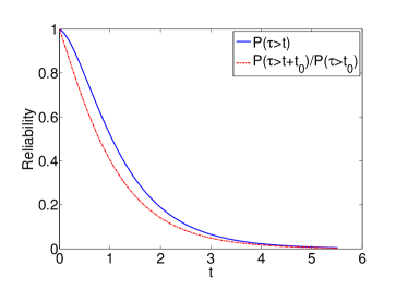
Figure 1: Example 13, NBU case

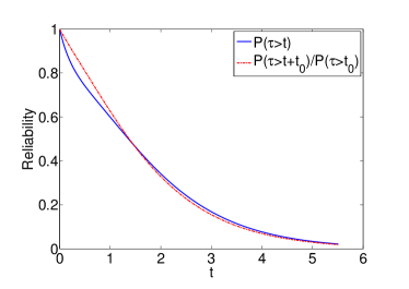
Figure 2: Example 13, not NBU case

Example 14

We here consider two extreme cases for the dependency between $V^{\left(1\right)}$ and $V^{(2)}$: independent or completely dependent (here $V^{\left(1\right)}=V^{(2)}$). The reliability in the completely dependent case is always greater than in the independent case (Fig. 3). This result is coherent with Proposition 10.

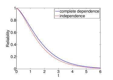
Figure 3: Comparison of reliability for two different types of dependence between $V^{(1)}$ and $V^{(2)}$, Example 14

Example 15

This example shows the monotony of the reliability with respect to the intensity of the Poisson process $\lambda\left(x\right)$ when $q$ is increasing, see Proposition 11. The more frequently the shocks occur, the lower the reliability is (Fig. 4).

Figure 4: Comparison of reliability for two different $\lambda\left(x\right)$, Example 15

7 Concluding remarks

We here proposed a random shock model with competing failure modes, which enlarges several models from the previous literature. The model takes into account different types of dependence between competing failures modes, where the dependence is induced by a common external shock environment. The reliability has been calculated by several different methods and conditions have been provided under which the system lifetime is New Better than Used. Due to this ageing property, it might be of interest to propose and study some maintenance policy to enlarge the system lifetime. Several versions might be proposed, according to the available information.

Also, the influence of the characteristics of the stressing environment on the lifetime $\tau$ has been studied. As expected, we saw that the lifetime was stochastically increasing with the probability $q\left(\cdot\right)$ for a shock to be non fatal. Besides, and that result was not necessarily so clear at first sight, we saw that the lifetime was also stochastically increasing with the dependence between the two marginal shock sizes. Finally, in case of a non decreasing function $q\left(\cdot\right)$, we saw that the lifetime was stochastically decreasing with the cumulated frequency of shocks. This means that the more frequent the shocks occur, the shorter the lifetime is. This result is natural but our proof is limited to the case of a non decreasing function $q\left(\cdot\right)$. In the special case of Cha and Mi (2011), the survival function of $\tau$ is however given by

$$\mathbb{P}(\tau>t)=e^{-H(t)-\int_{0}^{t}\left(1-\tilde{\mu}_{1}(t-w)q(w)\right)\lambda(w)~{}dw}$$

and it is easy to check that if $\lambda\geq\tilde{\lambda}$ (stronger assumption than $\Lambda\geq\tilde{\Lambda}$) then $\tau\leq_{st}\tilde{\tau}$, without any special condition on $q\left(\cdot\right)$. So, the stochastic monotonicity of the lifetime with respect of the (cumulated ?) frequency of shocks might be true under a more general setting than in the present paper, without assuming any monotonicity condition on $q\left(\cdot\right)$. We however have not been able to conclude on this point, and whether it is true or not remains an open question.

Acknowledgement 16

Both authors thank the referees for their carefull reading of the paper and their constructive remarks, which lead to a better introduction and justification of the model, and to a clearer paper. This work has been initiated during Hai Ha PHAM’s PhD studies in Pau (France), and has been supported by the Conseil Régional d’Aquitaine (France). This work has also been supported for both authors by the French National Research Agency (AMMSI project, ref. ANR 2011 BS01-021).

References

- A-Hameed and Proschan (1973) M. S. A-Hameed and F. Proschan. Nonstationary shock models. Stochastic Processes and their Applications, 1(4):383–404, 1973.
- A-Hameed and Proschan (1975) M. S. A-Hameed and F. Proschan. Shock models with underlying birth process. Journal of Applied Probability, 12(1):18–28, 1975.
- Brown and Proschan (1983) M. Brown and F. Proschan. Imperfect repair. Journal of Applied Probability, 20(4):851–859, 1983.
- Cha and Finkelstein (2009) J. H. Cha and M. Finkelstein. On a terminating shock process with independent wear increments. Journal of Applied Probability, 46(2):353–362, 2009.
- Cha and Mi (2007) J. H. Cha and J. Mi. Study of a stochastic failure model in a random environment. Journal of Applied Probability, 44(1):151–163, 2007.
- Cha and Mi (2011) J. H. Cha and J. Mi. On a stochastic survival model for a system under randomly variable environment. Methodology and Computing in Applied Probability, 13(3):549–561, 2011.
- Çinlar (2011) Erhan Çinlar. Probability and stochastics, volume 261 of Graduate texts in Mathematics. Springer Science + Business Media, 2011.
- Cocozza-Thivent (1998) C. Cocozza-Thivent. Processus stochastiques et fiabilité des systèmes, volume 28 of Mathématiques et Applications. Springer, 1998.
- Esary et al. (1973) J. D. Esary, A. W. Marshall, and F. Proschan. Shock models and wear processes. The Annals of Probability, 1(4):627–649, 1973.
- Finkelstein and Cha (2013) M. Finkelstein and J. H. Cha. Stochastic modeling for reliability: Shocks, burn-in and heterogeneous populations. Springer Series in Reliability Engineering. Springer, London, 2013.
- Gut (2001) A. Gut. Mixed shock models. Bernoulli, 7(3):541–555, 2001.
- Gut and Hüsler (1999) A. Gut and J. Hüsler. Extreme shock models. Extremes, 2(3):295–307, 1999.
- Hao et al. (2013) H.-B. Hao, C. Su, and Z.-Z. Qu. Reliability analysis for mechanical components subject to degradation process and random shock with wiener process. In 19th International Conference on Industrial Engineering and Engineering Management, pages 531–543, 2013.
- Lehmann (2006) A. Lehmann. Degradation-threshold-shock models. Probability, Statistics and Modelling in Public Health, pages 286–298, 2006.
- Lehmann (2009) A. Lehmann. Joint modeling of degradation and failure time data. Journal of Statistical Planning and Inference, 139(5):1693 – 1706, 2009. Special Issue on Degradation, Damage, Fatigue and Accelerated Life Models in Reliability Testing.
- Lemoine and Wenocur (1985) A. J. Lemoine and M. L. Wenocur. On failure modeling. Naval Research Logistics Quarterly, 32(3):497–508, 1985.
- Mallor and Omey (2001) F. Mallor and E. Omey. Shocks, runs and random sums. Journal of Applied Probability, 38(2):438–448, 2001.
- Mallor and Santos (2003a) F. Mallor and J. Santos. Classification of shock models in system reliability. Monografías del Semin. Matem. García de Galdeano, 27:405–412, 2003a.
- Mallor and Santos (2003b) F. Mallor and J. Santos. Reliability of systems subject to shocks with a stochastic dependence for the damages. Test, 12(2):427–444, 2003b.
- Marshall and Shaked (1979) A.W. Marshall and M. Shaked. Multivariate shock models for distributions with increasing hazard rate average. The Annals of Probability, 7(2):343–358, 1979.
- Nakagawa (2007) T. Nakagawa. Shock and damage models in reliability theory. Springer Series in Reliability Engineering. Springer, London, 2007.
- Qian et al. (1999) C. Qian, S. Nakamura, and T. Nakagawa. Cumulative damage model with two kinds of shocks and its application to the backup policy. Journal of the Operations Research Society of Japan-Keiei Kagaku, 42(4):501–511, 1999.
- Savits (1988) T. H. Savits. Some multivariate distributions derived from a non-fatal shock model. Journal of Applied Probability, 25(2):383–390, 1988.
- Shaked and Shanthikumar (2006) M. Shaked and J. G. Shanthikumar. Stochastic orders. Springer Series in Statistics. Springer, 2006.
- Singpurwalla (1995) N. D. Singpurwalla. Survival in dynamic environments. Statistical Science, 10(1):86–103, 1995.
- Skoulakis (2000) G. Skoulakis. A general shock model for a reliability system. Journal of Applied Probability, 37(4):925–935, 2000.
- Wang and Gao (2014) H.W. Wang and J. Gao. A reliability evaluation study based on competing failures for aircraft engines. Eksploatacja i Niezawodnosc: Maintenance and Reliability, 16(2):171–178, 2014.
- Zhu et al. (2010) Y. Zhu, E.A. Elsayed, H. Liao, and L.Y. Chan. Availability optimization of systems subject to competing risk. European Journal of Operational Research, 202(3):781 – 788, 2010.