On the symmetry of the electronic density in the three-electron parabolic quantum dot

Abstract

The structure of the lowest states of a three-electron axially symmetric parabolic quantum dot in a zero magnetic field is investigated. It is shown that the electronic density of the quartet ${}^{4}S$-states possesses certain approximate symmetry which is best seen when using Dalitz plots as the visualization tool. It is demonstrated that the origin of that symmetry is caused by the symmetry of the potential energy in the vicinity of its minimum. The discovered symmetry could provide an insight into the problem of the separation of slow and fast variables in the Schrödinger equation for the axially or spherically symmetric quantum dots.

I Introduction

Symmetries play very important role in physics Fano and Rau (1996). For example, such fundamental physical principles as the energy, linear and angular momentum conservation laws are based on the symmetry of the space-time with respect to translations and rotations. These symmetries can be considered as “kinematical symmetries” rather that dynamical ones since the former are independent on the interparticle interaction. It turns out that every exactly solvable quantum-mechanical problem possesses some kind of dynamical symmetry. Apparently, such situations are rather rare and are well-studied. Examples include the harmonic oscillator Fock (1928); Jauch and Hill (1940); Lutzky (1978) and hydrogen atom problems Fock (1935); Landau and Lifshitz (1977).

In some cases, however, a quantum system may have approximate symmetries. The existence of approximate symmetries leads to significant simplification of the analysis of the problem. Approximate symmetries are hard to find since the operator of the corresponding symmetry transformation does not commute with the Hamiltonian Ushveridze (2017). Nevertheless, approximate symmetries have been found for such nonseparable problems as hydrogen atom in a uniform magnetic field Zimmerman et al. (1980) and doubly excited states of helium atom Rost and Briggs (1991). Recently, the approximate symmetries of the nodal lines of the lowest Bressanini et al. (2005); Bressanini and Reynolds (2005) and resonant doubly-excited states Rost et al. (1991) of the helium atom have been discovered.

In the present article the approximate symmetry of the wave functions of the three electrons subjected to the circularly symmetric parabolic potential possesses is found. This problem is of interest since it is relevant in the theoretical investigation of the electronic structure of quantum dots. These are semiconductor structures which can confine electrons Kouwenhoven et al. (2001). Therefore, they are often referred to as “artificial atoms” Reimann and Manninen (2002). The theoretical study of few-electron quantum dots allows one to analyze the role of electronic correlations in nanostructures Bao (1997); Macsym et al. (2000); Puente et al. (2004).

The electronic structure of quantum dots can often be described by the model in which electrons having an effective mass move in a parabolic confining potential Fang et al. (2007); Wen-Fang (2007); Mikhailov (2002). Quantum dots with one or two-electrons are comparatively simple to study since the corresponding theory can be developed using various analytical model approaches Puente et al. (2004); Simonovic and Nazmitdinov (2003). Theoretical investigations of many-electron quantum dots are much more complicated because they require solution of many-dimensional partial differential equations which cannot be done analytically. Few-electron quantum dots are particularly difficult to study as in this case the application of various mean field approximations cannot be justified.

Obviously, the three-electron parabolic quantum dots are the simplest few-electron objects to analyze. They were studied rather extensively during the last decades Egger et al. (1999); Mikhailov (2002); Simonovic (2006). In particular, much attention has been paid to the properties of the three-electron quantum dots in a magnetic field Taut (2009); Fang et al. (2007). In the mentioned papers the energy spectrum was calculated using various approaches and the structure of the electronic density was studied using pair-correlation functions. The latter, however, is not always appropriate as it could hide some interesting features of electronic density which are caused by triple correlations. In the three-body problem it is more instructive to analyze the structure of the electronic density directly, using some suitable set of internal variables. The treatment of the present article is based on the Dalitz-plot technique which is often used to analyze the angular distributions in three-body break-up processes in particle and molecular physics Dalitz (1953); Müller et al. (1999); Galster et al. (2005); Kalliakos et al. (2008).

The use of Dalitz plots for the visualization of the electronic density greatly simplifies the analysis of its symmetries. Below it is shown that the Dalitz plots corresponding to the ground (and lowest excited) quartet states of the three-electron parabolic quantum dots posses some approximate symmetry similar to that observed in the model of the break-up of a three-body rigid rotator Meremianin (2006). This symmetry means that, at a given value of the hyperradius which defines the overall “size” of the configuration triangle, the dependence of the electronic density on the area of that triangle is very much stronger than on its shape. The detailed analysis performed with the help of internal variables similar to “Dalitz-Fabri” coordinates Efros et al. (1982); Krivec (1998) explains the origin of the observed approximate symmetry (Sec. V). Namely, it is caused by the symmetry of the total potential in the vicinity of its local minimum. This symmetry can be uncovered by taking the power series expansion of the potential. For some particular values of the confinement strength the magnitude of the distortion of the symmetry is estimated in Sec. IV.

For the sake of brevity, numerical calculations were carried out only for states with zero orbital momentum including the ground states of the quantum dot in the absence of external fields.

II The Hamiltonian of the three-electron quantum dot

The Schrödinger equation for the three electrons moving in a two-dimensional parabolic quantum dot is

$$-\frac{\hbar^{2}}{2m_{e}}\left(\sum_{i=1}^{3}\Delta_{\mathbf{R}_{i}}+U\right)\,\Psi_{t}=E\,\Psi_{t},$$ (1)

$$U=\sum_{i=1}^{3}\frac{m_{e}\,\omega^{2}\,R^{2}_{i}}{2}+\sum_{i>j=1}^{3}\frac{e^{2}}{\epsilon\,|\mathbf{R}_{i}-\mathbf{R}_{j}|},$$ (2)

where $m_{e}$ is the effective electron mass and $\epsilon$ is the dielectric constant.

For the confinement potential given in (1) it is possible to separate out the motion of the c.m. of electrons by introducing two Jacobi vectors $\mathbf{r}_{1,2}$ as is shown in Fig. (1).

Figure 1: Jacobi vectors for the three-body system. $\mathrm{c.m.}_{23}$ is the c.m. of the electrons ${2}$ and ${3}$.

The kinetic energy operator in terms of Jacobi vectors can be written as

$$-\frac{\hbar^{2}}{2m_{e}}\sum_{i=1}^{3}\frac{\partial^{2}}{\partial\mathbf{R}_{i}^{2}}=-\frac{\hbar^{2}}{6m_{e}}\frac{\partial^{2}}{\partial\mathbf{R}_{c.m.}^{2}}-\frac{\hbar^{2}}{m_{e}}\frac{\partial^{2}}{\partial\mathbf{r}_{1}^{2}}-\frac{3\,\hbar^{2}}{4m_{e}}\frac{\partial^{2}}{\partial\mathbf{r}_{2}^{2}}.$$ (3)

The sum of squared lengths of the position vectors re-written via Jacobi vectors is diagonal,

$$R^{2}\equiv R_{1}^{2}+R_{2}^{2}+R_{3}^{2}=3R_{c.m.}^{2}+\frac{1}{2}r_{1}^{2}+\frac{2}{3}r_{2}^{2}.$$ (4)

It is convenient to introduce the mass-scaled Jacobi vectors by making the following replacements in (3) and (4):

$$\mathbf{r}_{1}\to\sqrt{2}\,\mathbf{r}_{1},\quad\mathbf{r}_{2}\to\sqrt{\frac{3}{2}}\,\mathbf{r}_{2}.$$ (5)

With these replacements the Schrödinger equation reads

$$(H_{c.m.}+H_{int})\,\Psi_{t}=E\,\Psi_{t},$$ (6)

where $H_{c.m.}$ is the Hamiltonian describing the motion of c.m. of three electrons,

$$H_{c.m.}=-\frac{\hbar^{2}}{6m_{e}}\frac{\partial^{2}}{\partial\mathbf{R}_{c}^{2}}+\frac{3m_{e}\,\omega^{2}\,R_{c.m.}^{2}}{2},$$ (7)

and $H_{int}$ is the Hamiltonian corresponding to the internal (relative) motion of electrons in the parabolic trap

$$H_{int}=-\frac{\hbar^{2}}{2m_{e}}\left(\Delta_{1}+\Delta_{2}\right)+\frac{m_{e}\,\omega^{2}\,(r_{1}^{2}+r_{2}^{2})}{2}+e^{2}\kappa\,U_{cl},$$ (8)

where $\Delta_{1,2}=\partial^{2}/\partial\mathbf{r}_{1,2}^{2}$, $\kappa=1/\epsilon$ and $U_{cl}$ denotes the Coulomb repulsion terms

$$U_{cl}=\frac{1}{\sqrt{2}\,r_{1}}+\frac{\sqrt{2}}{|\mathbf{r}_{1}+\mathbf{r}_{2}\sqrt{3}|}+\frac{\sqrt{2}}{|\mathbf{r}_{1}-\mathbf{r}_{2}\sqrt{3}|}.$$ (9)

Dividing the Schrödinger equation by $\hbar\omega$ it can be brought to dimensionless form by making the replacements $r_{1,2}\to r_{1,2}\sqrt{\hbar/(m_{e}\omega)}$. As a result, the Hamiltonian assumes the form

$$H_{int}=-\frac{\Delta_{1}+\Delta_{2}}{2}+\frac{r_{1}^{2}+r_{2}^{2}}{2}+R_{c}\,U_{cl},$$ (10)

where the variables $r_{1,2}$ are dimensionless and $R_{c}$ is the Coulomb strength parameter,

$$R_{c}=\frac{e^{2}\kappa}{\hbar}\sqrt{\frac{m_{e}}{\hbar\omega}}=\alpha\kappa\sqrt{\frac{m_{e}c^{2}}{\hbar\omega}},$$ (11)

where $\alpha$ is the fine structure constant. The numerical calculations were carried out with the effective electron mass $m_{e}=0.067m$ and $\kappa=12.4$, which correspond to GaAs, so that

$$R_{c}=\frac{3.443}{\sqrt{(\hbar\omega)_{\mathrm{mEv}}}}.$$ (12)

III Dalitz plots of the electronic density

According to (6) the total wave function $\Psi_{t}$ can be expressed as the product of the wave function $\Psi_{c.m}$ describing the motion of c.m. of three electrons and the wave function $\Psi$ describing the relative motion of electrons:

$$\Psi_{t}=\Psi_{c.m.}(\mathbf{R}_{c.m})\,\Psi(\mathbf{r}_{1},\mathbf{r}_{2}).$$ (13)

The wave function $\Psi_{c.m.}$ has the same form as the wave function of a harmonic oscillator with the mass $3m_{e}$. It is the internal wave function which is determined by the electronic correlations. Therefore, below only the electronic density $D=|\Psi(\mathbf{r}_{1},\mathbf{r}_{2})|^{2}$ is considered.

In the three-electron quantum dot the density $D$ depends on three internal variables $\xi=(\xi_{1},\xi_{2},\xi_{3})$. Thus, $D(\xi)$ is a surface in the four-dimensional space and as such cannot be visualized. However, if we fix one of the internal variables, say $\xi_{1}$, then the function $D(\xi_{1}=const,\xi_{2},\xi_{3})$ becomes a three-dimensional surface which can be depicted on a sheet of paper as a color intensity map. Since the hyperradius $R$ is independent of the particle exchange, it is convenient to visualize $D(\xi)$ as a series of 3d surfaces with variable values of $R=0,\ldots,R_{max}$. Now the question is how to choose the two remaining internal variables to facilitate the features of the electronic density. Below we will use two dimensionless internal coordinates similar to those of a Dalitz plot.

Conventional Dalitz plots are the diagrams which depict the angular distributions of linear momenta of three particles Dalitz (1953); Müller et al. (1999). Originally, they were introduced to visualize the angular distributions of $K$ mesons in particle physics Dalitz (1953). On the Dalitz plot, each configuration of particle’s momenta is represented by the point inside a circle so that the exchange of particles is equivalent to the rotation by the angle $(2/3)\pi$ with respect to the center of the plot which itself corresponds to the equilateral configuration when vectors of particle’s momenta form an equal-side triangle. Points on the edge of the circle describe collinear configurations when particles fly apart along the same line.

To apply the Dalitz plot technique to the analysis of the electronic density we choose the coordinates of the polar plot to be the Dalitz coordinates Dalitz (1953); Fabri (1954) in the two-dimensional configuration space

$$x=\frac{R_{1}^{2}-R_{2}^{2}}{\sqrt{3}\,R^{2}},\quad y=\frac{1}{3}-\frac{R^{2}_{3}}{R^{2}}.$$ (14)

Here, it is assumed that c.m. of the three electrons is located at the origin of the coordinate frame, i.e.

$$\mathbf{R}_{c.m.}=\mathbf{R}_{1}+\mathbf{R}_{2}+\mathbf{R}_{3}=0.$$ (15)

The Dalitz coordinates (14) can also be expressed in terms of mass-scaled Jacobi vectors:

$$\begin{split}x&=\frac{1}{2\sqrt{3}\,R^{2}}\left(r_{2}^{2}-r_{1}^{2}-\frac{1}{\sqrt{3}}(\mathbf{r}_{1}\cdot\mathbf{r}_{2})\right),\\ y&=\frac{1}{6\,R^{2}}\left(r_{2}^{2}-r_{1}^{2}+2{\sqrt{3}}(\mathbf{r}_{1}\cdot\mathbf{r}_{2})\right),\end{split}$$ (16)

where the hyperradius $R=r_{1}^{2}+r_{2}^{2}$.

In literature are often used the symmetry adapted hyperspherical coordinates also known as “Dalitz-Fabri coordinates”, $R,a,\lambda$, Gronwall (1937); Efros et al. (1982); Krivec (1998); Badalyan and Simonov (1966) which are defined by the equations

$$\begin{split}r_{2}^{2}-r_{1}^{2}&=R^{2}\sin a\,\cos\lambda,\\ (\mathbf{r}_{1}\cdot\mathbf{r}_{2})&=\frac{R^{2}}{2}\sin a\,\sin\lambda,\end{split}$$ (17)

where $0\leq a\leq\pi/2$ and $0\leq\lambda\leq 2\pi$.

Note that the hyperangles $a,\lambda$ were, in fact, originally introduced by Gronwall and published in his posthumous paper Gronwall (1937) where the Hamiltonian of the helium atom Gronwall (1937) was written in terms of the variables $R,a,\lambda$. Therefore, below these coordinates will be referred to as “Gronwall-Dalitz-Fabri coordinates” (GDF).

Coordinates having similar kinematical properties as GDF coordinates $a,\lambda$, were used in molecular physics by several authors including Kuppermann Kuppermann (1975), Mead Mead (1992), Pack T Pack (1991). Mishra and Linderberg Mishra and Linderberg (1983) used Mead coordinates to visualize potential energy surfaces in triatomic molecules.

From (16), (17) one can deduce the connection of Cartesian coordinates $x,y$ to hyperangles $a,\lambda$,

$$\begin{split}x&=\frac{\sin\alpha}{3}\,\cos\left(\lambda+\frac{\pi}{6}\right),\\ y&=\frac{\sin\alpha}{3}\,\sin\left(\lambda+\frac{\pi}{6}\right),\end{split}$$ (18)

From these equations it follows that the polar radius $\rho$ on the Dalitz plot is

$$\rho\equiv\sqrt{x^{2}+y^{2}}=\frac{\sin a}{3}.$$ (19)

Using the identities (4), (14), (15) we obtain the representation of $\rho$ in terms of position vectors:

$$\rho^{2}=\frac{1}{9}-\frac{4\,|\mathbf{R}_{1}\times\mathbf{R}_{2}|^{2}}{3R^{4}}.$$ (20)

From (20) and (15) it is seen that the polar radius $\rho$ of the Dalitz plot is invariant under the particle exchange. This means that the exchange of particles is equivalent to the rotation or reflection of the diagram.

Expression (20) written in terms of Jacobi vectors has the form

$$\rho^{2}=\frac{1}{9}-\frac{4\,|\mathbf{r}_{1}\times\mathbf{r}_{2}|^{2}}{27R^{4}}.$$ (21)

The geometrical meaning of this equation is that polar radius of the Dalitz plot is determined by the ratio of the area $S$ of the configuration triangle and the hyperradius R:

$$\rho^{2}=\frac{1}{9}-\frac{16\,S^{2}}{27R^{4}}.$$ (22)

Indeed, the positions of particles define the vertices of the configuration triangle whose area is

$$S=\frac{1}{2}|\mathbf{r}_{1}\times\mathbf{r}_{2}|.$$ (23)

IV The numerical results

The wave function of the three electrons was obtained by diagonalizing the Hamiltonian (10) in the basis of Fock-Darwin states Darwin (1930); Fock (1928) which are defined by

$$\Psi_{n,m}(\mathbf{r}) = \frac{e^{-im\phi}}{\sqrt{2\pi}}\,\psi_{n,m}(r),$$ (24)

$$\psi_{n,m}(r) = \sqrt{\frac{n!}{(n+|m|)!}}\left(\frac{r}{\sqrt{2}}\right)^{|m|}e^{-r^{2}/4}L^{|m|}_{n}\left(\frac{r^{2}}{2}\right),$$ (25)

where $L^{|m|}_{n}$ is the associated Laguerre polynomial Erdelyi et al. (1953). Fock-Darwin wave functions (24) diagonalize the Hamiltonian of an electron in a parabolic circular trap. The corresponding single-electron energy is (in units of $\hbar\omega$)

$$E_{n,m}=(2n+1+|m|).$$ (26)

The expansion of the wave function of an $S$-state over the Fock-Darwin states has the form

$$\Psi(\mathbf{r}_{1},\mathbf{r}_{2})=\sum_{n=0}^{N}\sum_{n^{\prime}=0}^{N}\sum_{m=-m_{0}}^{m_{0}}F_{nn^{\prime},m}\,\Psi_{n,m}(\mathbf{r}_{1})\,\Psi_{n^{\prime},-m}(\mathbf{r}_{2}),$$ (27)

where $N$ and $m_{0}$ determine the accuracy of the representation of the wave function. The number of terms in the expansion (27) is

$$Z_{Nm_{0}}=(N+1)^{2}\,(2m_{0}+1).$$ (28)

The satisfactory convergence was achieved at $N,m_{0}\sim 5-7$. (Note that large values of $N,m_{0}$ lead to occurrence of spurious oscillations which degrades the accuracy of computations Haftel and Mandelzweig (1989).) Obtained results for the energy of the ground states are in good agreement with existing in literature Wen-Fang (2007).

Dalitz plots of the ground state electronic density $D_{0}=|\Psi_{0}(R,a,\lambda)|^{2}$ are given in Fig. 2 for the Coulomb strength parameter $R_{c}=5.444$ (which corresponds to the confinement energy $\hbar\omega=0.40$ meV) and two values of the hyperradius $R$. As is seen, the density has maximum at the center of the plot which is the equilateral configuration and decreases as the configuration triangle becomes more prolate, finally vanishing for collinear configurations.

The striking feature of the diagrams in Fig. 2 is the remarkably weak dependence of the density on the polar angle of the plot. In order to estimate the magnitude of this dependence, Fig. 3 shows the projection of the density $D_{0}(R,a,\lambda)$ on the surface $\lambda=const$ of the Cartesian frame with coordinates $(x_{1},x_{2},x_{3})=(a,\lambda,D_{0})$. The width of the curves shown in Fig. 3 is determined by the variation of the density as a function of the polar angle (which is actually $\lambda+\pi/6$, see (18)). The structure of the electronic density shown in Figs. 2,3 is preserved also for other values of the hyperradius $R$. For larger values of the confinement energy $\hbar\omega$ (which means smaller Coulomb parameter $R_{c}$) the electronic density has more pronounced maxima at the equilateral configuration. The calculations were also performed for other values of the confinement energy in the range $0.1$ – $0.4$ meV. In all cases the symmetry of the electronic density of the quartet states is essentially the same as in Figs. 2,3.

Note that at the values of the confinement energy $\hbar\omega\geq 0.62$ meV the ground state of the three-electron quantum dot is the doublet ${}^{2}P$-state with the total spin $S=1/2$ and the total orbital momentum $L=1$ Mikhailov (2002); Wen-Fang (2007). At $\hbar\omega=0.62$ meV the transition to the ground quartet ${}^{4}S$-state ($S=3/2$, $L=0$) occurs which is often referred to as the formation of the “Wigner molecule” Egger et al. (1999); Reusch et al. (2001); Macsym et al. (2000); Mikhailov (2002).

The Dalitz plots corresponding to the excited quartet states also have circular symmetry similar to that shown in Fig. 2. However, the computations of the wave functions for the excited states are less accurate than those of their eigenvalues and the corresponding results are not shown here.

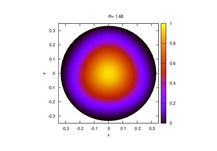
Figure 2: (Color online) The Dalitz plot for the electronic density of the ground state at the confinement energy $\hbar\omega=0.40$ meV ($R_{c}=5.444$) for two values of hyperradius $R$.

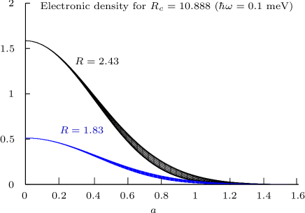
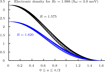
Figure 3: (Color online) Projections of the electronic density $D_{0}=|\Psi_{0}(R,a,\lambda)|^{2}$ of the quartet $S$-state on the plane $\lambda=const$ for three values of the Coulomb strength parameter $R_{c}$. Note that in the case of independence of the density on the hyperangle $\lambda$ the projections would be single thin lines.

V Expansion of the Coulomb energy and the origin of the symmetry

In terms of position vectors the potential energy of the electron-electron interaction in the quantum dot reads ($e=1$)

$$U=\frac{1}{R_{12}}+\frac{1}{R_{23}}+\frac{1}{R_{31}},$$ (29)

where $R_{ij}=|\mathbf{R}_{i}-\mathbf{R}_{j}|$.

According to Earnshaw’s theorem, the potential energy of the system of particles interacting via Coulomb forces cannot have minimum. However, in the case of electrons in a parabolic trap the equilibrium configurations can exist, i.e. there are minima of the total potential energy. Thus, we can expand the potential (29) in the vicinity of the equilibrium configuration. For example, the power series expansion of the first term on rhs of (29) can be written as

$$\frac{1}{R_{12}}=\sum_{k=0}^{\infty}\frac{1}{k!}((\mathbf{R}_{12}-\mathbf{R}_{12}^{(e)})\cdot\nabla)^{k}\,\frac{1}{r}\,\biggr{|}_{r=R^{(e)}_{12}}=\\ =\frac{1}{R^{(e)}_{12}}+\left(\frac{1}{R^{(e)}_{12}}-\frac{(\mathbf{R}_{12}\cdot\mathbf{R}_{12}^{(e)})}{{R^{(e)}_{12}}^{3}}\right)\\ +\left(\frac{1}{R^{(e)}_{12}}-\frac{R_{12}^{2}+4(\mathbf{R}_{12}\cdot\mathbf{R}_{12}^{(e)})}{2{R^{(e)}_{12}}^{3}}+3\frac{(\mathbf{R}_{12}\cdot\mathbf{R}_{12}^{(e)})^{2}}{2{R^{(e)}_{12}}^{5}}\right)+\ldots,$$ (30)

where $\mathbf{R}^{(e)}_{ij}$ is the position vector pointing from $i$-th to $j$-th electron at the equilibrium configuration. For the equilibrium configuration being an equilateral triangle we have that $R^{(e)}_{12}=R^{(e)}_{23}=R^{(e)}_{31}\equiv R_{e}$. If we take into account only zero- and first-order terms in the expansion (30) then the Coulomb potential (29) becomes

$$U=\frac{6}{R_{e}}-\frac{(\mathbf{R}_{12}\cdot\mathbf{R}_{12}^{(e)})+(\mathbf{R}_{23}\cdot\mathbf{R}_{23}^{(e)})+(\mathbf{R}_{31}\cdot\mathbf{R}_{31}^{(e)})}{R_{e}^{3}}.$$ (31)

We have to specify also the mutual orientation of the two configuration triangles, one built on equilibrium mutual vectors $\mathbf{R}_{12}^{(e)},\mathbf{R}_{23}^{(e)},\mathbf{R}_{31}^{(e)}$ and another one built on the instantaneous vectors $\mathbf{R}_{12},\mathbf{R}_{23},\mathbf{R}_{31}$. This can be done by using the moving frame which satisfies the Eckart condition Eckart (1935),

$$[\mathbf{R}_{12}^{(e)}\times\mathbf{R}_{12}]+[\mathbf{R}_{23}^{(e)}\times\mathbf{R}_{23}]+[\mathbf{R}_{31}^{(e)}\times\mathbf{R}_{31}]=0.$$ (32)

In terms of mass-scaled Jacobi vectors this equation reads

$$[\bm{\rho}_{1}\times\mathbf{r}_{1}]+[\bm{\rho}_{2}\times\mathbf{r}_{2}]=0.$$ (33)

where $\bm{\rho}_{1,2}$ are the equilibrium mass-scaled Jacobi vectors. As a result, the potential energy (31) assumes the form

$$U=\frac{6}{R_{e}}-3\,\frac{(\bm{\rho}_{1}\cdot\mathbf{r}_{1})+(\bm{\rho}_{2}\cdot\mathbf{r}_{2})}{R_{e}^{3}}.$$ (34)

In the Eckart frame the sum $(\bm{\rho}_{1}\cdot\mathbf{r}_{1})+(\bm{\rho}_{2}\cdot\mathbf{r}_{2})$ defines the Eckart parameter ${\cal F}$ which can be written as Meremianin (2004, 2013)

$${\cal F}=\sqrt{(\rho_{1}r_{1})^{2}+(\rho_{2}r_{2})^{2}+2\rho_{1}\rho_{2}r_{1}r_{2}\,\cos(\phi-\phi_{e})},$$ (35)

where $\phi_{e}$ is the angle between vectors $\bm{\rho}_{1}$ and $\bm{\rho}_{2}$. For the equilibrium configuration being an equilateral triangle we have that $\phi_{e}=\pi/2$ and $\rho_{1}=\rho_{2}=R_{e}/\sqrt{2}$ and the above identity becomes

$${\cal F}=R_{e}\sqrt{(r_{1}^{2}+r_{2}^{2})/2+r_{1}r_{2}\,\sin\phi}.$$ (36)

Using (17) one can derive the expression for the Eckart parameter in terms of GDF variables:

$${\cal F}=\frac{R_{e}R}{2}\sqrt{2+3\cos^{2}a}.$$ (37)

Thus, the potential energy (34) evaluates to

$$U=\frac{3}{2R_{e}}\left(4-\frac{R}{R_{e}}\sqrt{2+3\cos^{2}a}\right).$$ (38)

As is seen, the potential energy does not depend on the second hyperangle $\lambda$ and, hence, the dependence of the wave function on $\lambda$ is caused by the contribution of higher order terms in the expansion of the Coulomb potential (30). The results of numerical calculations presented above allows one to estimate the contribution of the higher-order multipoles in the expansion of Coulomb terms to be less than $10\%$ for the chosen values of the electron effective mass and the confinement strength.

VI Conclusion

In the presented article the symmetry of the electronic density of the circular parabolic three-electron quantum dots has been investigated. It is found that the electronic density (and the wave functions) of the quartet states depends on the shape of the configuration triangle much weaker than on its overall size and area. Such property of the density can be understood by employing the power (i.e. multipole) expansion of the total potential energy around the equilibrium configuration. The mentioned symmetry is best seen in the Dalitz diagrams for the electronic density (Sec. III). The Dalitz diagrams suggest that the internal variables most suited for the description of the problem are the Gronwall-Dalitz-Fabri coordinates $R,a,\lambda$ (see (17) of Sec. III) because among these coordinates the hyperangle $\lambda$ is the “slow variable” as it describes the shape of the configuration triangle.

Note that the approach employed above to explain the origin of the symmetry (Sec. V) is not limited to the case of planar quantum dots for which the numerical results were presented in Sec. IV. Thus, one can expect that some approximate symmetries similar to that uncovered in this article will show up in the three-dimensional case when three electrons are confined by an arbitrary spherically symmetric potential. Further, the consideration given in Sec. V can be easily generalized to the case of four- and more electrons which gives the possibility to distinguish slow and fast variables in the corresponding wave functions. This, however, needs more detailed investigations.

As to the physical background of the found weak dependence of the electronic density on the shape of the configuration triangle comparing to the dependence on its size and area, the quantum mechanical approach does not provide any obvious explanation. Perhaps, the semiclassical treatment would shed some light on the physical origin of the mentioned symmetry.

Another interesting problem would be to analyze the possible symmetry breaking caused, for example, by the influence of an external magnetic field. The application of the transversal magnetic field to a planar quantum dot does not violate the circular symmetry of the Hamiltonian and, therefore, should not change the symmetry drastically. However, if the magnetic field has components parallel to the plane of the quantum dot, then the symmetry of the electronic density will be broken. Finally, we note that effects of symmetry breaking in finite systems were recently reviewed in Birman et al. (2013).

References

- Fano and Rau (1996) U. Fano and A. R. P. Rau, “Symmetries in Quantum Physics” (Academic Press, 1996).
- Fock (1928) V. A. Fock, “Bemerkung zur Quantelung des harmonischen Oszillators im Magnetfeld”, Z. Phys. 47, 446 (1928).
- Jauch and Hill (1940) J. M. Jauch and E. L. Hill, “On the Problem of Degeneracy in Quantum Mechanics”, Phys. Rev. 57, 641 (1940), URL https://link.aps.org/doi/10.1103/PhysRev.57.641.
- Lutzky (1978) M. Lutzky, “Symmetry groups and conserved quantities for the harmonic oscillator”, Journal of Physics A: Mathematical and General 11, 249 (1978), URL http://stacks.iop.org/0305-4470/11/i=2/a=005.
- Fock (1935) W. Fock, “Zur Theorie des Wasserstoffatoms”, Z. Phys. 98, 145 (1935).
- Landau and Lifshitz (1977) L. D. Landau and E. M. Lifshitz, “Quantum mechanics” (Pergamon, New-York, 1977).
- Ushveridze (2017) A. G. Ushveridze, “Quasi-exactly solvable models in quantum mechanics” (Routledge, 2017).
- Zimmerman et al. (1980) M. L. Zimmerman, M. M. Kash, and D. Kleppner, “Evidence of an Approximate Symmetry for Hydrogen in a Uniform Magnetic Field”, Phys. Rev. Lett. 45, 1092 (1980), URL https://link.aps.org/doi/10.1103/PhysRevLett.45.1092.
- Rost and Briggs (1991) J. M. Rost and J. S. Briggs, “Saddle structure of the three-body Coulomb problem; symmetries of doubly-excited states and propensity rules for transitions”, Journal of Physics B: Atomic, Molecular and Optical Physics 24, 4293 (1991), URL http://stacks.iop.org/0953-4075/24/i=20/a=004.
- Bressanini et al. (2005) D. Bressanini, G. Morosi, and S. Tarasco, “An investigation of nodal structures and the construction of trial wave functions”, J. Chem. Phys. 123, 204109 (2005).
- Bressanini and Reynolds (2005) D. Bressanini and P. J. Reynolds, “Unexpected Symmetry in the Nodal Structure of the He Atom”, Phys. Rev. Lett. 95, 110201 (2005).
- Rost et al. (1991) J. M. Rost, R. Gersbacher, K. Richter, J. S. Briggs, and D. Wintgen, “The nodal structure of doubly-excited resonant states of helium”, Journal of Physics B: Atomic, Molecular and Optical Physics 24, 2455 (1991), URL http://stacks.iop.org/0953-4075/24/i=10/a=004.
- Fang et al. (2007) A. Fang, X. Chi, and P. Sheng, “Ground and excited states of three-electron quantum dots”, Solid State Communications 142, 551 (2007), ISSN 0038-1098, URL http://www.sciencedirect.com/science/article/pii/S0038109807002232.
- Wen-Fang (2007) X. Wen-Fang, “Three-Electron Quantum Dots in Zero Magnetic Field”, Communications in Theoretical Physics 48, 1115 (2007), URL http://stacks.iop.org/0253-6102/48/i=6/a=030.
- Mikhailov (2002) S. A. Mikhailov, “Quantum-dot lithium in zero magnetic field: Electronic properties, thermodynamics, and Fermi liquid–Wigner solid crossover in the ground state”, Phys. Rev. B 65, 115312 (2002).
- Kouwenhoven et al. (2001) L. P. Kouwenhoven, D. G. Austing, and S. Tarucha, “Few-electron quantum dots”, Reports on Progress in Physics 64, 701 (2001), URL http://stacks.iop.org/0034-4885/64/i=6/a=201.
- Reimann and Manninen (2002) S. M. Reimann and M. Manninen, “Electronic structure of quantum dots”, Rev. Mod. Phys. 74, 1283 (2002), URL https://link.aps.org/doi/10.1103/RevModPhys.74.1283.
- Bao (1997) C. G. Bao, “Large Regions of Stability in the Phase Diagrams of Quantum Dots and the Associated Filling Factors”, Phys. Rev. Lett. 79, 3475 (1997).
- Macsym et al. (2000) P. A. Macsym, H. Imamura, G. P. Mallon, and H. Aoki, “Molecular aspects of electron correlation in quantum dots”, J. Phys. Condens. Matter 12, R299 (2000).
- Puente et al. (2004) A. Puente, L. Serra, and R. G. Nazmitdinov, “Roto-vibrational spectrum and Wigner crystallization in two-electron parabolic quantum dots”, Phys. Rev. B (Condensed Matter and Materials Physics) 69, 125315 (pages 9) (2004), URL http://link.aps.org/abstract/PRB/v69/e125315.
- Simonovic and Nazmitdinov (2003) N. S. Simonovic and R. G. Nazmitdinov, “Hidden symmetries of two-electron quantum dots in a magnetic field”, Phys. Rev. B 67, 041305 (2003).
- Egger et al. (1999) R. Egger, W. Häusler, C. H. Mak, and H. Grabert, “Crossover from Fermi Liquid to Wigner Molecule Behavior in Quantum Dots”, Phys. Rev. Lett. 82, 3320 (1999), URL http://link.aps.org/doi/10.1103/PhysRevLett.82.3320.
- Simonovic (2006) N. S. Simonovic, “Three Electrons in a Two-Dimensional Parabolic Trap: The Relative Motion Solution”, Few-Body Systems 38, 139 (2006).
- Taut (2009) M. Taut, “Distortion of Wigner molecules: a pair function approach”, Journal of Physics: Condensed Matter 21, 075302 (2009), URL http://stacks.iop.org/0953-8984/21/i=7/a=075302.
- Dalitz (1953) R. H. Dalitz, “On the analysis of -meson data and the nature of the -meson”, Philos. Mag 44, 1068 (1953).
- Müller et al. (1999) U. Müller, T. Eckert, M. Braun, and H. Helm, “Fragment Correlation in the Three-Body Breakup of Triatomic Hydrogen”, Phys. Rev. Lett. 83, 2718 (1999).
- Galster et al. (2005) U. Galster, F. Baumgartner, U. Müller, H. Helm, and M. Jungen, “Experimental and quantum-chemical studies on the three-particle fragmentation of neutral triatomic hydrogen”, Phys. Rev. A 72, 062506 (2005).
- Kalliakos et al. (2008) S. Kalliakos, M. Rontani, V. Pellegrini, C. P. Garcia, A. Pinczuk, G. Goldoni, E. Molinari, L. N. Pfeiffer, and K. W. West, “A molecular state of correlated electrons in a quantum dot”, Nat. Phys. 4, 467 (2008), URL http://dx.doi.org/10.1038/nphys944.
- Meremianin (2006) A. V. Meremianin, “The Kinematical Model of the Sudden Break-up of the Three-Body Rigid Rotator”, Few-body Systems 38, 199 (2006).
- Efros et al. (1982) V. D. Efros, A. M. Frolov, and M. I. Mukhtarova, “Hyperspherical and related expansions in the Coulomb three-body problem”, Journal of Physics B: Atomic and Molecular Physics 15, L819 (1982), URL http://stacks.iop.org/0022-3700/15/i=23/a=001.
- Krivec (1998) R. Krivec, “Hyperspherical-harmonics methods for few-body problems”, Few-Body Systems 25, 199 (1998).
- Fabri (1954) E. Fabri, “A study of -meson decay”, Il Nuovo Cimento (1943-1954) 11, 479 (1954), ISSN 1827-6121, 10.1007/BF02781042, URL http://dx.doi.org/10.1007/BF02781042.
- Gronwall (1937) T. H. Gronwall, “The Helium Wave Equation”, Phys. Rev. 51, 655 (1937), URL http://link.aps.org/doi/10.1103/PhysRev.51.655.
- Badalyan and Simonov (1966) A. Badalyan and Y. Simonov, “Three-Body Problem: Equation For Partial Waves”, Yadern. Fiz. 3 (1966).
- Kuppermann (1975) A. Kuppermann, “A useful mapping of triatomic potential energy surfaces”, Chemical Physics Letters 32, 374 (1975), ISSN 0009-2614, URL http://www.sciencedirect.com/science/article/pii/0009261475851487.
- Mead (1992) C. A. Mead, “The geometrical phase in molecular systems”, Rev. Mod. Phys. 64, 51 (1992).
- T Pack (1991) R. T Pack, “Conformally euclidean internal coordinate space in the quantum three-body problem”, Chem. Phys. Lett. 230, 223 (1991).
- Mishra and Linderberg (1983) M. Mishra and J. Linderberg, “Hyperspherical representations of triatomic energy surfaces”, Molecular Physics 50, 91 (1983).
- Darwin (1930) C. G. Darwin, “The diamagnetism of the free electron”, Proc. Camb. Phil. Soc. 27, 86 (1930).
- Erdelyi et al. (1953) A. Erdelyi, W. Magnus, F. Oberhettinger, and F. G. Tricomi, “Higher trancendental functions. Bateman manuscript project”, vol. II (McGraw-hill book company, Inc, 1953).
- Haftel and Mandelzweig (1989) M. Haftel and V. Mandelzweig, “Fast convergent hyperspherical harmonic expansion for three-body systems”, Annals of Physics 189, 29 (1989).
- Reusch et al. (2001) B. Reusch, W. Häusler, and H. Grabert, “Wigner molecules in quantum dots”, Phys. Rev. B 63, 113313 (2001), URL https://link.aps.org/doi/10.1103/PhysRevB.63.113313.
- Eckart (1935) C. Eckart, “Some Studies Concerning Rotating Axes and Polyatomic Molecules”, Phys. Rev. 47, 552 (1935).
- Meremianin (2004) A. V. Meremianin, “Body frames in the separation of collective angles in quantum N-body problems”, J. Chem. Phys. 120, 7861 (2004).
- Meremianin (2013) A. Meremianin, “Eckart frame Hamiltonians in the three-body problem”, Journal of Mathematical Chemistry 51, 1376 (2013), ISSN 0259-9791, URL http://dx.doi.org/10.1007/s10910-013-0152-9.
- Birman et al. (2013) J. L. Birman, R. G. Nazmitdinov, and V. Yukalov, “Effects of symmetry breaking in finite quantum systems”, Physics Reports 526, 1 (2013), URL http://dx.doi.org/10.1016/j.physrep.2012.11.005.