Data-Oblivious Graph Algorithms
in Outsourced External Memory

Abstract

Motivated by privacy preservation for outsourced data, data-oblivious external memory is a computational framework where a client performs computations on data stored at a semi-trusted server in a way that does not reveal her data to the server. This approach facilitates collaboration and reliability over traditional frameworks, and it provides privacy protection, even though the server has full access to the data and he can monitor how it is accessed by the client. The challenge is that even if data is encrypted, the server can learn information based on the client data access pattern; hence, access patterns must also be obfuscated. We investigate privacy-preserving algorithms for outsourced external memory that are based on the use of data-oblivious algorithms, that is, algorithms where each possible sequence of data accesses is independent of the data values. We give new efficient data-oblivious algorithms in the outsourced external memory model for a number of fundamental graph problems. Our results include new data-oblivious external-memory methods for constructing minimum spanning trees, performing various traversals on rooted trees, answering least common ancestor queries on trees, computing biconnected components, and forming open ear decompositions. None of our algorithms make use of constant-time random oracles.

1 Introduction

Outsourced external memory is a computational framework where a client performs computations on data stored at a semi-trusted server. This approach facilitates reliability over traditional frameworks, but it also introduces a challenge with respect to privacy, since the server has full access to the data and he can monitor how it is accessed by the client. That is, a client outsources her data to an external server administered by a third party so that she can reliably access her data from anywhere using any computational device. Moreover, the client gains these features of reliability and availability often at very low cost (sometimes they are even free). Unfortunately, this approach introduces a loss of privacy that can occur from outsourcing data to a third party. Indeed, some cloud storage companies have based their business models on their ability to mine client data for useful information. Even if data is encrypted, information can be leaked from the way it is accessed. For example, Chen et al. [5] are able to infer sensitive information from the access patterns of popular health and financial web sites even if the data streams are encrypted. Thus, it is useful to design methods that allow for privacy-preserving access to data in the cloud. We are therefore interested in privacy-preserving algorithms for outsourced external memory that are based on the use of data-oblivious algorithms, that is, algorithms where each possible sequence of data accesses is independent of the data values. Such algorithms are useful for computation on outsourced data, since combining them with a semantically-secure encryption scheme will not reveal data values nor data access patterns.

In this paper, we work within the data-oblivious outsourced external memory (DO-OEM) model, which is our name for the model used in recent papers on algorithms and systems for data-oblivious outsourced storage solutions (e.g., see [4, 8, 10, 14, 17, 24, 26, 25, 30]). We assume that a large data set of size $N$ is stored on a server, who we will call “Bob,” and that a client, “Alice,” has access to this data through an I/O interface that allows her to make read and write requests of Bob using messages of size $B$ as atomic actions. We also assume Alice has a small amount of secure, private working memory, of size $M=\Omega(\log N)$.

The server, Bob, is “honest-but-curious,” which means that he will correctly perform every task requested, but he will also try to learn as much as possible about Alice’s data. This, of course, introduces privacy constraints for the DO-OEM model not found in the traditional I/O model (such as in [6]). In particular, we can rely on Bob to faithfully execute read and write requests, but he would like to learn as much as possible about Alice’s data. Thus, Alice must encrypt her data and then decrypt it and re-encrypt it with each read and write request, using a semantically-secure encryption scheme. Alice can safely perform any computation in her private memory, but her sequence of data accesses on the server must also not leak information about her data. That is, it must be data oblivious. The access sequence may depend on the function being computed, but it should be independent of the input data values.

Formally, we suppose Alice wants to perform an algorithm, $A$, which computes some function, $f$, on her data stored with Bob. In the context of graph algorithms, the input to $f$ is a graph, usually formatted as an array of edges, with $V$ and $E$ being the number of the graph’s vertices and edges, respectively. The output of $f$ may either be a property of the graph, such as whether or not the graph is biconnected, or another graph, such as a spanning tree, which will also be stored with Bob. Alice performs the algorithm $A$ by issuing read and write requests to Bob.

We say that $A$ is data-oblivious and can compute $f$ in the DO-OEM model if every probabilistic polynomial time adversary has only a negligable advantage over random guessing in a input-indistinguishability game.

1. The challenger sends a description of $f$ and $A$ to the adversary.

2. The adversary performs some computation, possibly including simulating $A$ on a polynomial number of inputs. The adversary chooses some input parameters and chooses an input satisfying the parameters. The adversary sends the input array and input parameters to the challenger.

3. The challenger generates an input satisfying the input parameters uniformly at random. The challenger flips a fair coin to decide whether to use the input provided by the adversary or to use the randomly generated input array. The challenger encrypts the selected input, and writes the encrypted array to a shared location.

4. The challenger runs algorithm $A$ on the shared encrypted array.

5. The adversary observes the sequence of reads and writes to the encrypted array, but does not see the challenger’s private memory or the unencrypted values of data in the array. After polynomial computation, the adversary guesses which input was used by the challenger. The adversary wins the game if it guesses correctly, otherwise the challenger wins.

Given a function $f$ and public input parameters (e.g. an upper bound on the size of the graph), $\gamma$, the probability that an algorithm to compute $f$ in the DO-OEM model executes a particular access sequence $S$ must be equally likely for any two inputs $X,Y$ satisfying parameters $\gamma$. That is, $P(S|f,\gamma,X)=P(S|f,\gamma,Y)$, or, from the Bob’s perspective, $P(X|f,\gamma,S)=P(Y|f,\gamma,S)$. We can achieve data-obliviousness if, knowing the size of the input, the function being computed, and the access sequence, all inputs are equally likely.

Moreover, for the problems we study in this paper, we would like to avoid using constant-time random oracles, since the existence of such functions is considered a strong assumption in the cryptographic literature (e.g., see [7]).

We use notation similar to the standard external memory model [29], but standard external memory techniques will not lead to data oblivious algorithms. Thus, although we measure the running time of our algorithm in I/Os, we require novel techniques in order to achieve data oblivious algorithms.

Previous Related Results.

Oblivious algorithms are discussed in a classic book by Knuth [18], and Pippenger and Fischer [22] show how to simulate a one-tape Turing machine of length $n$ with an oblivious two-tape Turing machine computation of length $O(n\log n)$. Goldreich and Ostrovsky [11] introduce the oblivious RAM model and show that an arbitrary RAM algorithm can be simulated (in internal memory) with an overhead of $O(\log^{3}N)$ through the use of constant-time random oracles, and this has subsequently been improved (e.g., see [12, 13, 15, 14]), albeit while still using constant-time random oracles. Ajtai [2] shows how to perform oblivious RAM simulation with a polylogarithmic factor overhead without constant-time random oracles and Damgård et al. [7] show how to perform such a simulation with an $O(\log^{3}N)$ overhead without using random oracles.

Chiang et al. [6] study (non-oblivious) external-memory graph algorithms and Blanton et al. [3] give data-oblivious algorithms for breadth-first search, single-source-single-target shortest paths and minimum spanning tree with running time $O(v^{2})$, and maximum flow with running time $O(v^{3}E\log V)$. However, their approach is based on computations on the adjacency matrix of the input graph, and thus only optimal on very dense graphs, whereas our approach is based on reductions to sorting the edge list, and is efficient on graphs of all densities.

Finding minimum spanning trees is a classic, well-studied algorithmic problem with many applications. Likewise, computing an st-numbering is vital in a number of graph drawing and planarity testing algorithms, and st-numbering in the data-oblivious model was listed as an open problem [16]. Thus, designing efficient DO-OEM algorithms for these problems can result in improved privacy-preserving algorithms for a number of other problems.

Our Results.

Let $\operatorname{DO-Sort}\left({N}\right)$ denote the number of I/Os required to sort an input of size $N$ in the DO-OEM model. For instance, Goodrich and Mitzenmacher [12] show $\operatorname{DO-Sort}\left({N}\right)=O((N/B)\log_{M/B}^{2}(N/B))$ I/Os, assuming $M>3B^{4}$. We develop efficient algorithms in the DO-OEM model for a number of fundamental graph problems:

• We show how to construct a minimum spanning tree of a graph $G$ in time depending on the input parameters $V$, $E$, density, and class of $G$, in the DE-OEM model: If $G$ belongs to a minor-closed family of graphs, such as a planar graph or any graph with bounded genus, then the run-time is $O(\operatorname{DO-Sort}\left({E}\right))$.

  Density	Class	Running Time	Constants
  $E=O(V\log^{\gamma}V)$	Any	$O(\operatorname{DO-Sort}\left({E}\right)\log V/\log\log V)$	$\gamma\geq 0$
  $E=\Theta(V2^{\log^{\delta}V})$	Any	$O(\operatorname{DO-Sort}\left({E}\right)\log^{1-\delta}V)$	$0<\delta<1$
  $E=\Omega(V^{1+\epsilon})$	Any	$O(\operatorname{DO-Sort}\left({E}\right))$	$0<\epsilon\leq 1$
  Any	Minor Closed	$O(\operatorname{DO-Sort}\left({E}\right))$	—

• Given a tree $T$, we can perform any associative traversal computation over $T$ in $O(\operatorname{DO-Sort}\left({V}\right))$ time in the DO-OEM model.

• Given a tree $T=(V,E)$ and a set, $S$, of pairs of vertices, we can compute the LCA, the least common ancestor, for each pair in $S$ in $O(\operatorname{DO-Sort}\left({|S|+V}\right))$ time in the DO-OEM model.

• Given a graph $G$ and a spanning tree of $G$, we can compute the biconnected components of $G$ in $O(\operatorname{DO-Sort}\left({E}\right))$ time in the DO-OEM model.

• Given a biconnected graph $G$, and a spanning tree of $G$, we can construct an open ear decomposition in $O(\operatorname{DO-Sort}\left({E}\right))$ time in the DO-OEM model.

• Given a biconnected graph $G$ and its open ear decomposition, we can find an st-numbering of $G$ in $O(\operatorname{DO-Sort}\left({E}\right))$ time in the DO-OEM model.

None of our algorithms use constant-time random oracles. Instead, they are based on a number of new algorithmic techniques and non-trivial adaptations of existing techniques.

2 Data-Oblivious Algorithm Design

2.1 Preliminaries

As is common in external memory graph algorithms we denote the input graph $G=(V,E)$, and slightly abuse notation by letting $V=|V|$ and $E=|E|$ when the context is clear. All logs are base 2 unless otherwise indicated. We use $[V]$ to denote the set of integers in the range $[1,|V|]$, and use $T$ to denote a rooted spanning tree of $G$. For each $v\in V$, $d(v)$ denotes the depth of $v$, i.e. the distance from the root in $T$. The parent of each node with respect to $T$ is denoted by $p(v)$. Let $T_{v}$ denote the subtree rooted at $v$, size$(v)$ denote the number of vertices in $T_{v}$, and preorder$(v)$ and postorder$(v)$ denote the order of $v$ in a preorder and postorder traversal of $T$ respectively. For each pair of nodes $u,v\in V$, $\operatorname{LCA}(u,v)$ denotes the least common ancestor of $u$ and $v$ in $T$.

Given a graph $G=(V,E)$ and an edge $(s,t)\in E$, an st-Numbering of $G$ is a function $\ell:V\to[V]$ which assigns integer labels to $V$ such that $s$ is labeled $\ell(s)=1$, $t$ is labeled $\ell(t)=V$, and every other vertex $v$ is adjacent to two vertices $u$ and $w$ such that $\ell(u)\leq\ell(v)\leq\ell(w)$.

An ear decomposition of $G$ is a partition of $E$ into a set of simple paths $P_{0},P_{1},\ldots P_{k}$ called ears such that $P_{0}=(s,t)$ and for each ear $P_{j}$, the internal vertices are disjoint from all $P_{i}$ where $i<j$, but each endpoint $L(P_{j})$ and $R(P_{j})$ of $P_{j}$ is either contained in $P_{0}$ or the internal vertices of some ear $P_{i}$, $0<i<j$. An ear $P_{i}$ is open if $L(P)\neq R(P)$ and an ear decomposition is open if all its ears are open.

We assume that the input is formatted as a list of $V$ vertices and $E$ directed edges sorted in adjacency list order. Note that we can organize an arbitrary list of edges into this order with $O(1)$ rounds of compressed-scanning. Although the edge list does not have separate storage for the vertices of the graph, for brevity, we sometimes say that we will store a data value at a vertex. However, to associate any data with a vertex, we must store that data in each edge incident to the vertex. It requires $O(1)$ rounds of compressed-scanning to distribute this data to all the incident edges.

2.2 ORAM Simulation

There are existing methods for simulating any random-access machine (RAM) algorithm (in internal memory) in a data-oblivious way without the use of random oracles. The best such oblivous RAM (ORAM) simulation method [7] which avoids constant-time random oracles, costs $O(\log^{3}N)$ per memory access, however. Thus, it is ideal if we can avoid using such general simulation results as much as possible. Therefore, in this paper, we are interested in methods for solving fundamental graph problems directly in the DO-OEM model.

2.3 Compressed Scanning

Compressed-Scanning.

Goodrich et al. [16] introduced compressed-scanning as a data-oblivious algorithm design technique for internal memory. Another related model is the massive, unordered, distributed (MUD) model for map-reduce [9]. We extend compressed-scanning to the DO-OEM model, and we use an algorithm design technique, where an algorithm is formulated so that it processes the input in a series of $t$ rounds as follows:

1. Scan each item of input exactly once; a random permutation hides the access pattern.

   • Read a block of $B$ items from input, possibly including some dummy items.

   • Perform some computation in private memory.

   • Write a block of $B$ items to output, possibly including some dummy items.

2. Sort the output data-obliviously.

3. Truncate the output, ignoring a portion, $L(i,\gamma)$, of the items, which may depend on the index of the round $i$ and input parameters $\gamma$ (e.g. input size), but not on any data values. For example, $L$ could be $0$ (no items are discarded) or $N/2^{i}$ (the last half of the output is discarded in each round).

4. Use the output as input for the next round.

This pattern is similar to the streaming model augmented with a sorting primitive [1].

Theorem 2.1.

Let $A$ be any compressed-scanning algorithm for which $t$ and $B$ depend only on $N$. Let $N_{i}$ denote the size of the input passed to round $i$. Then, $A$ can be simulated in the DO-OEM model in $O(\sum_{i=1}^{t}\operatorname{DO-Sort}\left({N_{i}}\right))$ time without the use of constant-time random oracles.

Proof.

By definition, we can run $A$ in the DO-OEM model if and only if $A$ satisfies the input-indistinguishability game. The algorithm runs in $t$ rounds, and each round has three phases: scan, sort, and truncate. The adversary can win the game if in any round, in any phase, the sequence of memory accesses to the shared encrypted array is different with non-negligible probability between the adversary’s input and input generated uniformly at random. However, by construction, the distribution of memory access by $A$ is the same at every phase for all inputs with the same input parameters. In the scan phase, each item of input is accessed once and in random order, regardless of the actual input values. Thus the scan phase conveys no advantage to the adversary. In the sorting phase, the sequence of memory access is likewise independent of the data values by definition, since we use a data-oblivious sorting algorithm. Hence, the sorting phase also conveys no advantage to the adversary. Finally, in the truncate phase, the portion of memory the algorithm chooses to ignore depends on the input parameters, but will be identical, regardless of whether the input is the one chosen by the adversary or the one generated uniformly at random. So the truncate phase also conveys no advantage to the adversary. In every phase of every round, the adversary gains no information as to which input was chosen by the coin toss. Therefore, every probabilistic polynomial time adversary has a negligable advantage over random guessing. The running time is a straightforward sum of the cost to data-obliviously sort the input in each round. ∎

As we explore in this paper, using this design approach results in much improved running times over a general RAM-simulation approach. Thus, we would like to use compressed-scanning algorithms as much as possible. This approach introduces some interesting challenges from an algorithmic perspective, and designing efficient compressed-scanning algorithms for even well-known problems often involves new insights or techniques (e.g., see [16]).

3 Tree-Traversal Computations

Many traditional graph algorithms are based on a traversal of a spanning tree of the graph, for example, using depth first search. However, the data access pattern of depth first search fundamentally depends on the structure of the graph, and it is not clear how to perform DFS efficiently in the DO-OEM model. Instead, we use Euler Tours [27], adapted for data-oblivious tree-traversal computation [16]. Given an undirected rooted tree $T$, we imagine that each edge $\{p(v),v\}$ is composed of two directed edges $(p(v),v)$ and $(v,p(v))$, called an advance edge and retreat edge respectively. An Euler tour of $T$ visits these directed edges in the same order as they would be visited in a depth first search of $T$. However, an Euler tour implemented with compressed-scanning does not reveal information to the adversary because each data item is accessed once and in random order.

We give more details concerning the implementation of an Euler tour in Appendix A. Let E-order$(u,v)$ denote the order of the edge $(u,v)$ in an Euler tour of $T$. Note that $\texttt{preorder}(v)=\texttt{E-order}(p(v),v)$ and $\texttt{postorder}(v)=\texttt{E-order}(v,p(v))$.

Some tree statistics are straightforward to compute using Euler Tours. For example, Goodrich et al. [16] show how to compute the size of the subtree for each node $v\in T$ using an Euler Tour and compressed-scanning pass over the edges of $T$. The calculation is straightforward once we observe that $\texttt{size}(v)=(\texttt{E-order}(v,p(v))-\texttt{E-order}(p(v),v))/2+1$, since for each proper descendant of $v$, we will traverse one advance edge and one retreat edge. Thus, the number of edges traversed between $(p(v),v)$ and $(v,p(v))$ is twice the number of proper descendants of $v$, and we add one to also include $v$ in $\texttt{size}(v)$. Moreover, Euler tour construction can be done data-obliviously in external memory in $O(\operatorname{DO-Sort}\left({|T|}\right))$ I/Os by a data-oblivious compressed-scanning implementation of the algorithm by Chiang et al. [6].

However, Euler-Tours are insufficient to compute most functions where the value at a vertex is dependent on its parent or children. Therefore, in the following, we describe more sophisticated techniques for tree traversal computations, suitable for computing functions in which the value at a vertex depends on its parent or children.

3.1 Bottom-Up Computation.

Let $T$ be a tree rooted at $r$. First, we show how to compute recursive functions on the vertices bottom up using a novel data-oblivious algorithm inspired by the classic parallel tree contraction of Miller and Reif [21]. Like Miller and Reif’s algorithm, our algorithm compresses a tree down to a single node in $O(\log V)$ rounds. However, unlike the original algorithm, we are able to compress long paths of degree two nodes into a single edge in a single iteration and guarantee the size of the graph decreases by half in each round.

Each round of the tree contraction algorithm is divided into two operations: rake, which removes all the leaves from $T$, and compress, which compresses long paths by contracting edges for which the parent node only has a single child.

First, we label each vertex with its degree by scanning the edge list in adjacency list order. Then, for each vertex $v\neq r$, if $v$ has degree 1, it is a leaf, and it is marked for removal by the rake operation. Otherwise, if it has degree 2, then it is marked for contraction by the compress operation. The marks are stored with the endpoints of each edge.

Now, we perform the rake operation via an Euler tour of $T$. For each unmarked edge we read, we write back its value unchanged. If an advance edge is marked as a leaf, then we mark the edge for removal. The next edge we read is the corresponding retreat edge from the leaf. We evaluate the leaf and output the computed value together with the label of the parent vertex instead of the original retreat edge. Next we distribute this information to the other incident edges; we sort the edge list so that for each vertex we first see all the evaluated leaves and then see the remaining outgoing edges. In a compressed scanning pass we are able to store the function evaluation from each leaf in its parent. Thus we complete the rake operation.

Figure 1: A single round of the rake and compress operations on a small example graph.

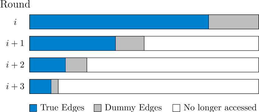
Figure 2: The portion of memory accessed by the algorithm decreases by a constant fraction in each round.

Next, we perform the compress operation via another Euler tour of $T$. We remove each marked advance edge by writing dummy values in its place. For each retreat edge to a degree two node, we contract the edge by composing the functions at the parent and child and storing this value in private memory. For all but the last edge in a path of degree two nodes, we mark the edge for removal. For the last edge in the path, we output the label of the parent vertex together with the composition of all functions along the path. Although the path may not have constant size, for the functions considered in this paper (such as min), the composition across values of nodes along the path can be expressed in $O(1)$ space by partially evaluating the function as we go. We pass this information to other edges incident to the last vertex in the path, for all the compressed paths, using a single compressed scanning round. Thus, we complete the compress operation. (See Figure 2.)

Finally, we perform one last compressed scanning pass to set aside all edges marked for removal. These edges are placed at the end of the list by the sort and are not required for subsequent processing. Thus we complete one round of the algorithm. However, we may continue to access some dummy edges in subsequent rounds so that in round $i+1$ we always access a constant fraction of the memory accessed in round $i$, thus maintaining the data-oblivious property of our algorithm (see Figure 2).

We now analyze the total time it takes to contract a tree down to the root node. Each round of rake and compress on a tree $T_{i}$ of size $V_{i}$ takes $O(\operatorname{DO-Sort}\left({V_{i}}\right))$ time to perform $O(1)$ Euler tours and compressed scanning rounds. We begin with an initial tree $T_{0}=T$ of size $V_{0}=V$. Without loss of generality, we can partition the nodes of any tree $T_{i}$ into three sets: $B_{i}$, the branch nodes with at least $2$ children; $P_{i}$, the path nodes with $1$ child; and $L_{i}$, the leaf nodes. Clearly $|B_{i}|+|P_{i}|+|L_{i}|=V_{i}$, and $|L_{i}|\geq 2|B_{i}|$. The rake operation removes all of $L_{i}$, and all but at most one node in each path in $P_{i}$. Thus, $V_{i+1}\leq|B_{i}|+\frac{1}{2}|P_{i}|<\frac{1}{2}(3|B_{i}|+|P_{i}|)\leq\frac{1}{2}V_{i}$. Hence, $\sum_{i}V_{i}$ is a geometric sum, and the total running time of all rounds is $O(\operatorname{DO-Sort}\left({V}\right))$.

Throughout the algorithm the children of each branch and leaf node are finalized before we process the node. However, some path nodes may have been compressed and set aside before all of their descendants were finalized. Thus, in a final post-processing step, we perform one more round of compressed scanning and Euler tour over the full edge list to finalize the value of the internal path nodes.

Computation of low.

Suppose we are given a spanning tree $T$ of a graph $G$. We illustrate rake and compress by computing the following simple recursive function.

$$\texttt{low}(v)=\min( \{\texttt{preorder}(v))\}$$

$$\cup\{\texttt{low}(w)\mid\mbox{ $w$ is a child of $v$ in $T$}\}$$

$$\cup\{\texttt{preorder}(w)\mid(v,w)\in G-T\})$$

That is, for each vertex $v\in T$, $\texttt{low}(v)$ is the lowest preorder number of a vertex that is a descendant of $v$ in $T$, or adjacent to a descendant via a non-tree edge. This function is a key part of the biconnected components algorithm, and key functions in our other algorithms are computed similarly.

First, we compute the preorder numbers of each vertex by an Euler tour of $T$. Next, we preprocess the edge list. In $O(1)$ compressed-scanning rounds, we compute for each vertex the minimum preorder number between that vertex and all its neighbors in $G-T$. We store this data in the endpoints of each edge $(u,v)$ in the edge list as the initial values for $\texttt{low}(u)$ and $\texttt{low}(v)$. This preprocessing requires $O(\operatorname{DO-Sort}\left({E}\right))$ time.

Now, we use rake and compress to compute the recursive portion of low. Each iteration of rake and compress proceeds as follows. The low value of each leaf is already finalized. We store $\texttt{low}(v)=\min\left(\{\texttt{low}(v)\}\cup\{\texttt{low}(w)\mid w\text{ is a child of }v\}\right)$ as the function for each internal node $v$. When we rake a leaf $\ell$, we update its parent $p$, $\texttt{low}(p)=\min(\texttt{low}(p),\texttt{low}(\ell)).$ During the compress step, when we contract an edge $(p(v),v)$ we update the function stored at in $p(v)$ as follows: $\texttt{low}(p(v))=\min(\texttt{low}(p(v)),\texttt{low}(v))$, and $\texttt{children}(p(v))=\texttt{children}(v)$. Note that vertex may have many children, but always a single parent. Thus, the easiest way to change the assignment of children is to set $\texttt{label}(p(v))=\texttt{label}(v)$ and then relabel the edge $(p(p(v)),p(v))$ = $(p(p(v)),v)$. We may need to perform this relabeling and calculation of low over a long path, but we always process nodes bottom up, and we maintain the values of the previous edge processed in private memory. We output dummy values for all but the final edge in the path, which stores the minimum low of the whole path, together with the labels of the first and last vertex on the path. Finally, we synchronize each edge with the new values of its endpoints via compressed-scanning, which completes the iteration of rake and compress. After at most $O(\log V)$ iterations and $O(\operatorname{DO-Sort}\left({V}\right))$ I/Os, we complete the rake and compress algorithm. Thus, the preprocessing time dominates, and the total time required to compute low for all vertices is $O(\operatorname{DO-Sort}\left({E}\right))$.

3.2 Top-down computation

We now show how to run our compression algorithm “in reverse” in order to efficiently compute top-down functions where each vertex depends on the value of its parent. First, we simulate the compression algorithm described above, and label each edge $e$ with contract$(e)$, the order in which it would have been removed from the graph. Thus, all edges incident to leaves in the initial graph are given a label smaller than any interior nodes, and all edges incident to the root are given larger labels than edges incident to nodes of depth $>1$.

Next, we sort the edges in reverse order according to their contract labels. We process the edges in this order in $\lceil\log V\rceil$ stages. We mark the root as finished. Then, in each stage $i$, we perform the following on the first $2^{i}$ edges in the sorted order: For each advance edge $e=(p(v),v)$, if $p(v)$ is marked as finished, we evaluate the function at $v$, augment $e$ with its value, and mark $v$ as reached. Between stages $i$ and $i+1$, we process the first $2^{i+1}$ edges, and distribute the new values at reached vertices from the previous stage to any incident edges belonging to the next stage. Finally, we mark each reached vertex as finished. Thus, the function at a parent is always evaluated before the function at its children, and each child edge has been augmented with the value from the parent before the edge is processed.

Each stage requires $O(1)$ rounds of compressed scanning. Since the number of edges processed in each stage is $2^{i}$, the running time of the final stage dominates all other stages, and thus the total time is $O(\operatorname{DO-Sort}\left({V}\right))$. Note that since our algorithm essentially reduces to data-oblivious sorting and compressed scanning, the sequence of data accesses made by the algorithm are independent of the input values. Thus, no probabilistic polynomial adversary has more than negligible advantage in the input-indistinguishability game. We summarize our results in the following theorem:

Theorem 3.1.

Given a tree $T$, we can perform any top-down or bottom-up tree-traversal computation over $T$ in $O(\operatorname{DO-Sort}\left({V}\right))$ time in the DO-OEM model.

LCA computation.

Suppose we are given a connected graph $G=(V,E)$ and a spanning tree $T=(V,E_{T})$ of $G$ rooted at $t$. We can preprocess $G$ and augment each edge $(u,v)\in E$ with additional information such that we can find the least common ancestor $\operatorname{LCA}(u,v)$ with respect to $T$ in constant time. Given two integers $x,y$, let $\texttt{rzb}(x)$ denote the number of rightmost zero bits in the binary representation of $x$, and let $x\&y$ denote the bitwise logical AND of $x$ and $y$. The following preprocessing algorithm is adapted from the parallel algorithm of Schieber and Vishkin [23].

For each node $v\in T$, we compute preorder$(v)$, and size$(v)$. We also set $\texttt{inlabel}(v)$ to $\max_{w\in T_{v}}\texttt{rzb}(\texttt{preorder}(w))$, that is, the maximal number of rightmost zero bits of any of the preorder numbers of the vertices in the subtree rooted at $v$. As in our computation of low in Section 3.1, we can compute these functions via rake and compress together with a $O(1)$ Euler tour and compressed-scanning steps so that each edge $(u,v)\in G$ stores the augmented information associated with its endpoints. We also initialize $\texttt{ascendent}(t)=2^{\lfloor\log V\rfloor}$.

We compute $\texttt{ascendant}(v)$ for each vertex $v\in V$ as follows: If $\texttt{inlabel}(v)$ is equal to $\texttt{inlabel}(p(v))$, then set $\texttt{ascendent}(v)$ to $\texttt{ascendent}(p(v))$. Otherwise, set $\texttt{ascendent}(v)$ to $\texttt{ascendent}(p(v))+2^{i}$, where $i=\log(\texttt{inlabel}(v)-[\texttt{inlabel}(v)\&(\texttt{inlabel}(v)-1)])$ is the index of the rightmost non-zero bit in $\texttt{inlabel}(v)$. Thus, ascendent is a top-down function, and we can evaluate it at all nodes in the tree in $O(\operatorname{DO-Sort}\left({V}\right))$ time using the method of Section 3.2.

Finally, we perform an Euler-Tour traversal to compute a table head. We set $\texttt{head}(\texttt{inlabel}(v))$ to be the vertex of minimum depth $d(u)$ among all the vertices $u$ such that $\texttt{inlabel}(u)=\texttt{inlabel}(v)$ on the path from the $t$ to $v$ in $T$. Note that since there are at most $\log V$ distinct inlabel numbers, the size of head is at most $O(\log V)$ and can fit in private memory. By a constant number of compressed-scanning steps, we store $\texttt{head}(\texttt{inlabel}(u))$ and $\texttt{head}(\texttt{inlabel}(v))$ with each edge $(u,v)\in G$.

Given the additional information now stored in each edge, we can compute the $\operatorname{LCA}(u,v)$ for any edge $(u,v)\in G$ in constant time by a few simple algebraic computations as shown by Schieber and Vishkin [23].

We summarize this result in the following theorem:

Theorem 3.2.

Given a tree $T$ and a set of pairs of vertices $S\subset V\times V$, we can compute $\operatorname{LCA}(u,v)$ for all $u,v\in S$ in $O(\operatorname{DO-Sort}\left({|S|+V}\right))$ time in the DO-OEM model.

4 Minimum Spanning Tree

In this section we present a novel algorithm to compute the minimum spanning tree of a general graph in the DO-OEM model. Our algorithm has additional input parameters of the density and class of the graph, and its running time depends on these parameters. Thus, our algorithm necessarily reveals asymptotically the vertex and edge counts, and whether the input graph is minor-closed. However, revealing this information does not convey any advantage to the adversary in the input-indistinguishability game. In fact, these input parameters can be freely chosen by the adversary. Of course, if we don’t want to allow these input parameters and the corresponding gains in efficiency, we can avoid revealing this information by working with an adjacency matrix instead of an edge list, or we can also achieve a tradeoff between privacy and efficiency by padding the input with dummy edges.

In the case of somewhat dense graphs, or graphs from a minor closed family, our runtime is $O(\operatorname{DO-Sort}\left({E}\right))$. We conjecture that this is optimal since we require this time to perform even a single round of compressed scanning in our model. For graphs of other classes and densities, our algorithm still beats the previously best known method for computing any spanning tree in the DO-OEM model by logarithmic factors.

Our MST algorithm requires the following sub-routines: trim, select, contract and cleanup.

trim$(G,\alpha)$:
We scan the edge list of $G$ and trim the outgoing edges from each node, depending on the value of an input parameter $\alpha$. If the degree of a node is at most $\alpha$, then we leave its outgoing edges unchanged. If the degree of a node is less than $\alpha$, then we implicitly pad its outgoing edge list up to size $\alpha$ with additional dummy edges of weight $\infty$. However, if the degree of a node is greater than $\alpha$, then the node keeps its $\alpha$ smallest outgoing edges and discards the rest. For a given edge each endpoint independently chooses to keep or discard it as an outgoing edge. Note that we can trim the edge list in $O(1)$ rounds of compressed scanning. Afterwards, the graph may no longer be connected (see Figure 3).

select$(G)$:
Each node selects the minimum outgoing edge from its adjacency list. If two edges have the same weight, we break ties lexicographically. We mark the edges as selected as follows: First, sort the edges lexicographically by source vertex, weight. Then, in a single compressed scanning round we mark the minimum weight edge from each source vertex as selected. The set of selected edges partition $G$ into connected components, and in each connected component, one edge has been selected twice (see Figure 3). For each double-selected edge, we arbitrarily choose to keep one copy and mark the other as dummy. We can gather all the dummy edges to the end of the list in $O(1)$ compressed scanning rounds. The output is a spanning forest of $G$ such that in each tree all the edges are oriented from the root to the leaves.

contract$(G,E_{s})$:
The input is a graph $G$ and a set of selected edges $E_{s}$ which induce a spanning forest $F\subseteq G$. For each connected component in $F$, we merge the nodes in the component into a single pseudo-node by contracting all the selected edges in that component (Figure 3). Using our top-down tree-traversal algorithm, we re-label each node with the label of the root of its component. Then, in two compressed scanning rounds we relabel the endpoints of the all edges in $G$ to reflect the relabeled nodes, possibly creating loops and parallel edges. In the first round we relabel the source for each outgoing edge of each node. In the second round we sort the edges to group them by incoming edges with each node, and relabel the target for each edge. In a final oblivious sort, we restore the edge list of $G$ to adjacency list (lexicographical) order.

cleanup$(G)$:
We detect and remove duplicate, parallel and loop edges in a single compressed-scanning round. When we encounter parallel edges, we remove all but the minimum weight edge between two nodes. As we scan the edge list, we remove an edge by writing a dummy value in its place, and then we perform a final oblivious sort to place all the dummy values at the end of the list.

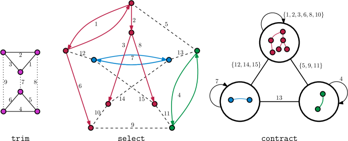
Figure 3: Left: the result of trim on a small example graph with $\alpha=2$. Removed edges are denoted by dotted lines. Center and Right: the result of select and contract on a small example graph. In select, unselected edges are dashed, and selected edges are solid and oriented towards the vertex which selected them. The selected edges form a spanning forest of $G$; each connected component is a tree in which one edge has been selected twice. In contract, each connected component is contracted to a single pseudo-node.

Minimum Spanning Forest (MSF).

Let $G_{0}=\texttt{trim}(G,\alpha)$ for an appropriate choice of parameter $\alpha$ to be discussed later. Then, the core of our algorithm is as follows: for $i\in[1,\alpha]$, let

$$G_{i}=\texttt{trim}(\texttt{cleanup}(\texttt{contract}(G_{i-1},\texttt{select}(G_{i-1}))),\alpha).$$

That is, we perform $\alpha$ iterations in which we select the minimum edge out of each node, contract the connected components, “remove” unwanted edges from the resulting graph by labeling them as dummies, and pass the cleaned and trimmed graph to the next iteration. Each subsequent iteration accesses a constant fraction of the memory accessed in the previous iteration, possibly including some dummy edges (see Figure 2). In a final pass, we contract and cleanup all the edges of $G$ with respect to the connected components represented by the nodes of $G_{\alpha}$.

Throughout our algorithm, the set of selected edges induce a spanning forest of $G$. Each pseudo-node represents an entire tree in this forest. We define a weight function $w(v)$ for each pseudo-node, which corresponds to the number of true nodes contained in the tree represented by the pseudo-node. Initially each node has weight 1.

At each trim step, we remove a subset of edges. The remaining edges induce a set of potential connected components $C_{1},\ldots,C_{t}$. For each $C_{i}$, let $w(C_{i})=\sum_{v\in C_{i}}w(v)$. We maintain the following invariant throughout all iterations of our algorithm: $w(C_{i})\geq\alpha$ for all $C_{i}$.

The invariant remains true after the initial trim step; we know that each $C_{i}$ contains at least $\alpha+1$ nodes, since $G$ was connected, and trim only removes edges from nodes of degree more than $\alpha$. Subsequent trim steps also maintain the invariant since nodes of degree $\leq\alpha$ are not effected and nodes of degree $>\alpha$ will still be connected to at least $\alpha$ other nodes after the trim.

Next, in the select step, each node selects one outgoing edge for contraction. For each edge $(u,v)$ that we contract in the contract step, we create a new pseudo-node $x$ of weight $w(x)=w(u)+w(v)$. Thus, the total weight of each $C_{i}$ does not change over the contract step. However, we select at least $|C_{i}|/2$ edges in each component. Thus, the number of nodes within each component $C_{i}$ is reduced by half.

The cleanup step only removes redundant edges, and does not effect the number of nodes or the weight in any components.

Hence, after $O(\log\alpha)$ iterations, the size of each $C_{i}$ is reduced by a factor of $\alpha$, and the total weight of each $C_{i}$ remains at least $\alpha$. Therefore, the resulting graph has at most $O(V/\alpha)$ pseudo-nodes.

We now consider the running time of the MSF algorithm. The first run of trim$(G)$ and the final pass both take $O(\operatorname{DO-Sort}\left({E}\right))$ time. Each sub-routine used in each iteration takes $O(\operatorname{DO-Sort}\left({|G_{i}|}\right))$ time. Moreover, for each $i$, $|G_{i+1}|\leq|G_{i}|/2$. Therefore, the time used in all iterations is a geometric sum, and the time required by all iterations is $O(\operatorname{DO-Sort}\left({|G_{0}|}\right))=O(\operatorname{DO-Sort}\left({\alpha\cdot V}\right))$. Hence, the total running time of one repetition of MSF is $O(\operatorname{DO-Sort}\left({E}\right)+\operatorname{DO-Sort}\left({\alpha\cdot V}\right))$. Moreover, we can repeat our algorithm $k$ times to achieve the following result. Let $G^{j}(\alpha)$ denote the graph for the $j$th repetition of the MSF algorithm with parameter $\alpha$, that is, the graph consisting of the pseudo-nodes (subsets of vertices of $G$) from the output of the previous iteration, and the $\alpha$ smallest edges out of each pseudo-node. The running time of $k$ repetitions is

$$\sum_{j=0}^{k-1}O(\operatorname{DO-Sort}\left({E}\right)+\operatorname{DO-Sort}\left({\alpha|G^{j}(\alpha)|}\right))$$

$$=O(k\cdot\operatorname{DO-Sort}\left({E}\right))+\sum_{j=0}^{k-1}O(\operatorname{DO-Sort}\left({\alpha\frac{V}{\alpha^{j}}}\right))$$

$$=O(k\cdot\operatorname{DO-Sort}\left({E}\right)+\operatorname{DO-Sort}\left({\alpha V}\right))$$

We require that the final output $|G^{k}(\alpha)|=1$ is a single pseudo-node representing a spanning tree of $G$, which implies that $k=\frac{\log V}{\log\alpha}$. Thus, we choose parameter

$$\alpha=\frac{\beta}{\log\beta}\mbox{, where }\beta=\frac{E\log V}{V}$$

to minimize the total running time, depending on the density of the graph. Hence, the running time is

$$O\left(\operatorname{DO-Sort}\left({E}\right)\frac{\log V}{\log\frac{\beta}{\log\beta}}+\operatorname{DO-Sort}\left({E\frac{\log V}{\log\beta}}\right)\right)$$

If the graph $G$ is somewhat dense with $E=\Omega(V^{1+\epsilon})$ for any arbitrarily small constant $\epsilon>0$, then this implies a running time of $O(\operatorname{DO-Sort}\left({E}\right))$. If $G$ has density $E=\theta(V2^{\log^{\delta}V})$, for any constant $0<\delta<1$ then this implies a running time of $O(\operatorname{DO-Sort}\left({E}\right)\cdot\log^{1-\delta}V)$. If $G$ is sparse with $E=O(V\log^{\gamma}V)$, for any constant $\gamma\geq 0$, then we achieve a running time of $O(\operatorname{DO-Sort}\left({E}\right)\cdot\log V/\log\log V)$. However, if $G$ is from a minor closed family, e.g. if it is a planar graph, we can be even more efficient and simplify our algorithm.

Mareš [20] gave a related algorithm in the standard RAM model (not data-oblivious). He showed that for any non-trivial minor closed families of graphs, a Borůvka-style round of edge contractions will always decrease the size of the graph by a constant factor. Therefore, we will have a similar geometric sum in the running time of our algorithm for any input graph drawn from a non-trivial minor closed family of graphs, including any graph with bounded genus.

Thus, in this case we do not need the trim sub-routine at all, since the size of the graph will be decreasing geometrically by the minor closed property. Then we run our algorithm with parameters $\alpha=E$ and $k=1$. Therefore, the total time required for all iterations is $O(\operatorname{DO-Sort}\left({E}\right))$. Furthermore, since we always selected the minimum edge out of each component, by the cut property of minimum spanning trees we are guaranteed that the algorithm produces a minimum spanning tree of $G$. Moreover, The algorithm makes choices depending on the input parameters but the fundamental components of our algorithm are data-oblivious sorting and compressed scanning and the memory access pattern never depends on the data values. Thus, no probabilistic polynomial time adversary has more than negligible advantage in the input-indistinguishability game.

We summarize our result in the following theorem:

Theorem 4.1.

In the DO-OEM model, we can construct a minimum spanning tree of a graph $G$ in time depending on the input parameters $V$, $E$, density, and class of $G$. If $G$ belongs to a minor-closed family of graphs, such as any graph with bounded genus, then the running time is $O(\operatorname{DO-Sort}\left({E}\right))$. We achieve the following run-times:

Density	Class	Running Time	Constants
$E=O(V\log^{\gamma}V)$	Any	$O(\operatorname{DO-Sort}\left({E}\right)\log V/\log\log V)$	$\gamma\geq 0$
$E=\Theta(V2^{\log^{\delta}V})$	Any	$O(\operatorname{DO-Sort}\left({E}\right)\log^{1-\delta}V)$	$0<\delta<1$
$E=\Omega(V^{1+\epsilon})$	Any	$O(\operatorname{DO-Sort}\left({E}\right))$	$0<\epsilon\leq 1$
Any	Minor Closed	$O(\operatorname{DO-Sort}\left({E}\right))$	—

Given the minimum spanning tree algorithm and tree-traversal computation technique outlined above, we can also achieve the following results for a biconnected graph. We can verify that a graph is biconnected or compute the biconnected components of a graph using the techniques described in Section 5.

5 Biconnected Components

Tarjan and Vishkin [27] gave an efficient sequential algorithm for computing the biconnected components of a graph. We rely on the correctness of their algorithm, but the details of each step are necessarily different in our data-oblivious biconnected components algorithm.

Suppose we are given a spanning tree $T$ of a graph $G$. Using our traversal computation method, we compute $\texttt{low}(v)$ for each vertex $v\in T$ as outlined in Section 3.1. We also compute a similar function $\texttt{high}(v)$, using identical techniques. The function high is the same as low except we recursively compute the $\max$ instead of $\min$ preorder number. We also compute for each vertex its preorder number, the size of its subtree and its grandparent in $T$ (if it exists).

After this preprocessing, we construct the following edge list of an auxiliary graph $G^{\prime\prime}$. Each vertex of $G^{\prime\prime}$ corresponds to an edge of $T$. We add edges to $G^{\prime\prime}$ as follows:

• For each edge $\{p(v),v\}\in T$, such that $\texttt{preorder}(v)\neq 1$, and
  either $\texttt{low}(v)\leq\texttt{preorder}(p(v))$ or $\texttt{high}(v)\geq p(v)+\texttt{size}(p(v))$,
  we add the edge $\{\{p(p(v)),p(v)\},\{p(v),v\}\}$ to $G^{\prime\prime}$.

• For each edge $\{v,w\}\in G-T$ such that
  $\texttt{preorder}(v)+\texttt{size}(v)\leq\texttt{preoder}(w)$,
  we add the edge $\{\{p(v),v\},\{p(w),w\}\}$ to $G^{\prime\prime}$.

Now, we find the connected components of $G^{\prime\prime}$ and label each edge of $T$ with the label of its component in $G^{\prime\prime}$ using the top-down tree-traversal computation technique of Section 3.2. Next, give each edge $\{v,w\}$ of $G-T$ with $\texttt{preorder}(v)<\texttt{preorder}(w)$ the label of edge $\{p(w),w\}$ in $T$ in $O(1)$ compressed scanning passes. Tarjan and Vishkin [27] showed the resulting component labels correspond exactly to the biconnected components of $G$. Thus, we can compute the biconnected components of $G$ in $O(\operatorname{DO-Sort}\left({E}\right))$ time. We summarize this result in the following theorem:

Theorem 5.1.

Given a graph $G$ and a spanning tree of $G$, we can compute the biconnected components of $G$ in $O(\operatorname{DO-Sort}\left({E}\right))$ time in the DO-OEM model.

6 Open Ear Decomposition

Let $T=(V,E_{T})$ be a spanning tree of $G$ rooted at $t$ such that there is only a single edge $(s,t)\in E_{T}$ incident to $t$. The edges of $E-E_{T}$ are denoted non-tree edges, and the edges $E_{T}-(s,t)$ are denoted tree edges. The edge $(s,t)$ is treated separately. Let $G$ be a biconnected graph.

We structure our algorithm around the same steps used by Maon et al. [19] in their parallel ear-decomposition algorithm. However, the details of each step are necessarily different in important ways as we show how to efficiently implement each step in the DO-OEM model.

1. Find a spanning $T$ of $G$ rooted at $t$ such that $(s,t)$ is the only edge incident to $t$. We remove the vertex $t$ from $G$ and run the above MST algorithm on $G[V-\{t\}]$ to get a set of edges $E^{\prime}$ which form a spanning tree of $V-\{t\}$. Let $E_{T}=E^{\prime}\cup(s,t)$. Then the desired spanning tree of $G$ is given by $T=(V,E_{T})$.

2. 1. For each tree edge $(u,v)\in E_{T}$, we compute $d(u)$, $d(v)$, $p(u)$ and $p(v)$ via an Euler-Tour traversal of $T$. We also preprocess $G$ using the LCA algorithm given in Corollary 3.2.

   2. Number the edges of $G$, assigning each $e\in E$ an arbitrary integer serial number $\texttt{serial}(e)\in[E]$. Define a lexicographic order on the non-tree edges $f$ according to $\texttt{number}(f)=\left(d(\operatorname{LCA}(f)),\texttt{serial}(f)\right)$

3. Each non-tree edge $f$ induces a simple cycle in $(V,E_{T}\cup f)$. We will adapt an algorithm of Vishkin [28] to compute compute a function $\texttt{master}(e)$ for each tree edge $e$.

   Fact 6.1.

   [19] Each non-tree edge $f$, together with the set of edges $e_{i}$ such that $\texttt{master}(e_{i})=f$ form a simple path or cycle, called the ear of $f$.

   Fact 6.2.

   [19] The lexicographical order on $\texttt{number}(f)$ over the non-tree edges induces an order on the ears, which yields an ear decomposition (which is not necessarily open).

   Fact 6.3.

   [19] Let $(u,v)$ be a non-tree edge. Let $x=\operatorname{LCA}(u,v)$. Let $e_{u}$ and $e_{v}$ be the first edges on the path from $x$ to $u$ and $v$ in $T$ respectively. Then, the ear induced by $(u,v)$ is closed if and only if $e_{u}$ and $e_{v}$ both choose $(u,v)$ as their master.

   As shown by Maon et al. [19], the resulting ear-decomposition is not necessarily open, and we must first refine the order defined on the edges. Therefore, we refine the ordering on non-tree edges sharing a common LCA by updating the assignment of serial with the following additional steps.

4. Construct a bipartite graph $H_{x}=(V_{x},E_{x})$ for each vertex $x\in V-\{t\}$. Each vertex in $V_{x}$ corresponds to an edge in $G$. Specifically, $V_{x}$ is the set of edges $(u,v)$ such that $x=\operatorname{LCA}(u,v)$. Note that this includes tree edges $(x,w)$ for which $x=p(w)$. Thus, the graphs $H_{x}$ partition the edges of $G$.

   There is an edge in $E_{x}$ between a tree edge $e$ and a non-tree edge $(y,z)$ if and only if $e$ is the first edge on the path from $x$ to $y$ or $z$ in $T$. There are no other edges in $E_{x}$. We can test all such edges by creating a list of each endpoint in $V_{x}$ sorted by preorder number. That is, all tree edges $(x,w)$ will appear once ordered by $\texttt{preorder}(w)$ and each non-tree edge $(y,z)$ will appear twice, once ordered by $\texttt{preorder}(y)$ and once ordered by $\texttt{preorder}(z)$. Then, each non-tree edge is incident to the first tree edge that comes before and after it according to the above ordering.

   We compute the set $E_{x}$ for all the graphs $H_{x}$ “in parallel”; that is, we do not require separate passes over the edge list of $G$ to compute each $H_{x}$. First, in $O(1)$ rounds of compressed scanning, we label each edge $e$ with $\operatorname{LCA}(e)$. Then, we sort the edge list by $\operatorname{LCA}(e),\texttt{E-order}(e)$. In an additional $O(1)$ rounds of compressed scanning, we compute $V_{x}$ and $E_{x}$ for each $H_{x}$.

5. Construct a spanning forest for each $H_{x}$. Note that each edge in $E$ appears in exactly one $H_{x}$, and that the degree of each non-tree node is at most $2$. Hence, the total size of all such graphs $H_{x}$ is $\theta(E)$. We construct all the spanning forests in two Borůvka-style rounds as follows. In the first round, each non-tree node in $V_{x}$ selects one of its incident edges. This results in a spanning forest. Then in a cleanup phase, we contract each connected component into a pseudo-node, and remove loops and duplicate edges between pseudo-nodes. In the second round, each non-tree node in $V_{x}$ selects its second edge (if present). We perform a second cleanup phase. The remaining selected edges form a forest consisting of a spanning tree over each connected component of each $H_{x}$. Clearly we can implement the selection and cleanup phases in a constant number of compressed-scanning rounds.

6. Fact 6.4.

   [19] For each connected component of each $H_{x}$, there exists at least one tree edge $e\in V_{x}$ such that $d(\operatorname{LCA}(\texttt{master}(e)))<d(x)$.

   In light of this fact, we do the following:

   1. For each connected component $C$ of each $H_{x}$, find such an edge $e$ guaranteed by the above fact and construct an Euler Tree $T_{C}$ over $C$ rooted at $e$.

   2. Compute the pre-order numbers preorder$(e)$ of each non-tree edge $e$ with respect to $T_{C}$ by performing an Euler tour traversal of $T_{C}.$

   3. Recall that the edges were ordered according to the number assigned above: $\texttt{number}(f)=\left(d(\operatorname{LCA}(f)),\texttt{serial}(f)\right)$. We reorder the non-tree edges by replacing their old serial numbers with the new preorder numbers as follows: $\texttt{newnumber}(f)=\left(d(\operatorname{LCA}(f)),\texttt{preorder}(f)\right)$.

7. Now we are ready to compute the assignment of master based on the new ordering of the non-tree edges. We proceed as follows:

   1. Compute $\texttt{preorder}(v)$ and $\texttt{postorder}(v)$ for each vertex $v\in V$ by an Euler Tour traversal of $T$.

   2. For each vertex $v$, let $E_{v}$ denote the set of non-tree edges incident to $v$. If $\operatorname{LCA}(E_{v})\neq v$, then let $(u,v)\in E_{v}$ be an edge such that $\operatorname{LCA}(u,v)=\operatorname{LCA}(E_{v})$. That is, the edge $(u,v)$ such that $d(\operatorname{LCA}(u,v))$ is minimized. If there is more than one such edge for a given vertex, choose a single edge arbitrarily.

      Assign a tuple $\texttt{serial}(u,v)=(d(\operatorname{LCA}(u,v)),\texttt{serial}(u,v))$ to each chosen edge $(u,v)$ combining the depth of the least common ancestor and its old serial number. Note that the edge $(u,v)$ can be found by scanning the adjacency list of $v$ in $E-E_{T}$ after the above LCA preprocessing. Thus, we can relabel the serial numbers of all chosen edges in a single compressed-scanning pass.

      As shown by Vishkin [28], all the non-tree edges that were not chosen in the previous step can be discarded for the remaining computation of master.

   3. For each tree edge $e=(p(v),v)$, initialize $\texttt{master}(e)=f$, where $f$ is the non-tree edge incident to $v$ with minimum serial number among the edges chosen in the previous step. Note that the initial assignment of master can be computed for all tree edges in a single scan after sorting the chosen edges and tree edges in adjacency list order.

   4. Perform a bottom-up traversal computation on $T$. For each tree edge $e=(p(v),v)$, we assign a new value for $\texttt{master}(e)=g$, where $g$ is the edge with minimum master$(g)$ among all the edges between $(p(v),v)$ and $(v,p(v))$ in the Euler Tour traversal of $T$.

Fact 6.5.

[19] The set of non-tree edges chosen as master partition the tree edges into the subsets that chose them. Each master edges induces an ear, and the ordering of the corresponding non-tree edges results in an open ear decomposition of $G$.

This fact, together with the above algorithm, give us the following theorem.

Theorem 6.6.

Given a biconnected graph $G$, and a spanning tree of $G$, we can construct an open ear decomposition in $O(\operatorname{DO-Sort}\left({E}\right))$ time in the DO-OEM model.

Proof.

There are a constant number of steps outlined above for computing the ear decomposition. It was already shown by Maon et al. [19] that completing these steps correctly yields a valid open ear decomposition. It remains to consider the time taken by each step. Each step involves a constant number of compressed scanning rounds and Euler tree traversals, which each take at most $O(\operatorname{DO-Sort}\left({E}\right))$ time. Therefore, the running time of the entire algorithm is $O(\operatorname{DO-Sort}\left({E}\right))$. Since the algorithm essentially reduces to data-oblivious sorting and compressed-scanning, no probabilistic polynomial adversary can have more than negligible advantage in the input-indistinguishability game. ∎

7 st-Numbering

At a high level, our algorithm for st-numbering is similar to the one given in [19]. That is, our algorithm is also structured in two stages; in the first stage, we orient each ear in the ear decomposition based on some simple rules, and in the second stage we compute the st-numbering by traversing the ears in an order based on their orientations. Necessarily the details of each stage are significantly different in the DO-OEM model.

The input to our st-numbering algorithm is an open ear decomposition, structured as a sequence of ears (edge disjoint paths) $P_{i}$, where $P_{0}=(s,t)$. Each ear $P_{i}$ has a left and right endpoint denoted $L(P_{i})$ and $R(P_{i})$ respectively. Each vertex in $P_{i}$ which is not an endpoint of $P_{i}$ is called an internal vertex of $P_{i}$. Note that each vertex in an internal vertex in exactly one ear. We say that a vertex is belongs to an ear only if it is an internal vertex of that ear. The endpoints of each ear other than $P_{0}$ belong to two (not necessarily distinct) ears which occur earlier in the sequence.

Since the algorithm numbers internal vertices based on the ear which contains them, we can safely ignore any ears (other than $P_{0}$) which do not contain any interior vertices. Thus, all single-edge ears other than $P_{0}$ are discarded, and the algorithm is only run on the remaining graph which has size $O(V)$.

We assume that each edge is augmented with the index of the ear which contains it and the index of the ear containing each endpoint. Furthermore each edge has a pointer to adjacent edges in the path, indicating whether the neighboring edge is towards $L(P)$ or $R(P)$. Finally, the internal vertices which belong to each ear are numbered according to the left to right order from $L(P)$ to $R(P)$, and each edge is augmented with the numbers of its endpoints. If needed, the augmentation can easily be computed with compressed-scanning steps.

7.1 Orientation

The vertex $L(P)$ is also called the anchor of ear $P$. There is a natural tree structure given by the ears and their anchors. The ear tree $ET$ is a directed tree rooted at $P_{0}$. It is formally defined as follows: Each ear $P_{i}$ is a vertex in $ET$. There is an edge $(P_{j},P_{i})$ for each pair of ears such that the anchor of $L(P_{i})$ of $P_{i}$ belongs to $P_{j}$. We say that vertex $u$ belonging to $P_{i}$ is a descendant of a vertex $v$ belonging to $P_{j}$ if $P_{i}$ is a descendant of $P_{j}$ in $ET$.

We construct $ET$ in a constant number of compressed scanning rounds. We number each edge in $ET$ according to its order in a preorder traversal of $ET$ via an Euler tour traversal. Then, we augment a set of non-tree edges $\{L(.),R(.)\}$. For each ear $P_{i}$, we precompute $\operatorname{LCA}(L(P_{i}),R(P_{i}))$ using the least common ancestor of Corollary 3.2. Let $e_{L}$ and $e_{R}$ be the first tree edge on the path from $\operatorname{LCA}(L(P_{i}),R(P_{i}))$ to $L(P_{i})$ and $R(P_{i})$ respectively. In a constant number of additional compressed scanning rounds, we store with each non-tree edge $\{L(P_{i}),R(P_{i})\}$ the data, including pre-order number and left-to-right number, associated with $e_{L}$ and $e_{R}$.

For each ear $P_{i}$, the orientation of $P_{i}$ depends only on the orientation previously assigned to some individual ear $P_{m}$, called the hinge of $P_{i}$. We say that an ear gets the same direction as its hinge if either both ears are oriented from $L(.)$ to $R(.)$ or both are oriented from $R(.)$ to $L(.)$. Otherwise, we say the ears get opposite directions.

The set of ears and their hinges also form a tree structure. The hinge tree $HT$ is formally defined as follows: Each ear $P_{i}$ is a vertex in $HT$. There is an edge $(P_{m},P_{i})$ for each pair of ears such that $P_{m}$ is the hinge of $P_{i}$. The hinge of each ear $P_{i}$ can be determined by a few constant time tests based on the information stored in $(L(P_{i}),R(P_{i}))$ during the above preprocessing phase. Details of these tests is given is Section 7.3. Given the hinges, we can build the hinge tree in a constant number of compressed scanning rounds. Finally, we can perform an Euler tour traversal of the hinge tree in order to determine the orientation of each ear.

7.2 Numbering

An ear oriented from right to left (towards its anchor) is called an incoming ear, and an ear oriented from left to right (away from its anchor) is called an outgoing ear. We define a total order on the ears based on their orientations. The internal order of incoming ears is the same as the order of the corresponding edges in $ET$, and the internal order of outgoing ears is opposite of the corresponding edges in $ET$. Each incoming ear is before each outgoing ear. Thus, we can compute the relative order of any two edges in constant time given their orientations. Hence, in $O(1)$ rounds of compressed scanning, we can compute the st-numbering, which yields the following theorem.

Theorem 7.1.

Given a biconnected graph $G$ and a spanning tree for $G$, we can find an st-numbering of $G$ in $O(\operatorname{DO-Sort}\left({E}\right))$ time in the DO-OEM model.

Proof.

As outlined above, the algorithm consists of an orientation phase and a numbering phase. We also need to perform some pre-processing of least-common-ancestors in the ear tree. Each phase requires at most a constant number of tree traversal computations. However, the input to each phase has size $O(V)$, since the algorithm initially discards any ears other than $(s,t)$ without internal nodes. Therefore, each phase has running time $O(\operatorname{DO-Sort}\left({V}\right))$ and the running time is dominated by the time required to discard the uninteresting ears, which is $O(\operatorname{DO-Sort}\left({E}\right))$.

Since the algorithm is composed of data-oblivious sorting and compressed-scanning, no probabilistic polynomial adversary can have more than negligible advantage in the input-indistinguishability game. ∎

7.3 Hinge Finding

We now describe how to find the hinge of each ear. The following is based on the case analysis of Maon et al. [19] and is included here for completeness. There are no significant differences in the assignment of orientation, and thus correctness follows. The primary differences are the extra care we need to take to efficiently maintain the data-oblivious property of our algorithm. This is handled by storing the necessary data with each ear $P_{i}$ during the above preprocessing of $(L(P_{i}),R(P_{i}))$.

There are two cases two consider.

1. If $L(P_{i})$ and $R(P_{i})$ belong to the same ear $P_{j}$, then $P_{j}$ is the hinge of $P_{i}$. We orient $P_{i}$ in the same direction as $P_{j}$ if and only if $L(P_{i})$ is left of $R(P_{i})$ in $P_{j}$.

   Let $e_{L}$ and $e_{R}$ be the edges in $P_{i}$ incident to $L(P_{i})$ and $R(P_{i})$ respectively. In constant time, we can test if $L(P_{i})$ and $R(P_{i})$ belong to the same ear by looking at the ear index of $L(P_{i})$ and $R(P_{i})$ stored in $e_{L}$ and $e_{R}$. We can also test in constant time whether $L(P_{i})$ is left of $R(P_{i})$ in $P_{j}$ by looking at the left-to-right numbering stored in $e_{L}$ and $e_{R}$.

2. If $L(P_{i})$ and $R(P_{i})$ belong to different ears $P_{j}$ and $P_{k}$ respectively, then there are several cases to consider. Let $P_{\alpha}$ be the LCA of $P_{j}$ and $P_{k}$ in $ET$.

   1. If $P_{\alpha}$ is distinct from $P_{j}$ and $P_{k}$, then let $v_{j}$ and $v_{k}$ be the anchor ancestors of $P_{j}$ and $P_{k}$ respectively. There are two cases to consider:

      1. If $v_{j}$ and $v_{k}$ are distinct (i.e. $v_{j}\neq v_{k}$), then $P_{\alpha}$ is the hinge of $P_{i}$. Similarly to case 1, we orient $P_{i}$ in the same direction as $P_{\alpha}$ if and only if $v_{j}$ is to the left of $v_{k}$ in $P_{\alpha}$.

      2. If $v_{j}=v_{k}$, then let $v=v_{j}=v_{k}$, and let $e_{j}=(v,P_{j^{\prime}})$ and $e_{k}=(v,P_{k}^{\prime})$ be the first edge on the path from $P_{\alpha}$ to $P_{j}$ and $P_{k}$ respectively. If $e_{j}$ comes before $e_{k}$ in the adjacency list from $v$, then the hinge of $P_{i}$ is $P_{j}^{\prime}$ and $P_{i}$ gets a direction opposite to $P_{j}^{\prime}$. Otherwise $P_{k}^{\prime}$ is the hinge of $P_{i}$, and $P_{i}$ gets the same direction as $P_{k}^{\prime}$. Given the information stored with $(L(P_{i}),R(P_{i})$ during the LCA preprocessing, we can determine the hinge of $P_{i}$ and whether it gets the same or opposite direction of its hinge in constant time.

   2. If $P_{\alpha}=P_{k}$, then let $v$ be the anchor ancestor of $P_{i}$ in $P_{\alpha}$.

      1. If $v\neq R(P_{i})$ then $P_{\alpha}$ is the hinge of $P_{i}$, and $P_{i}$ gets the same direction as $P_{\alpha}$ if $v$ is to the left of $R(P_{i})$ in $P_{\alpha}$.

      2. If $v=R(P_{i})$, then the hinge of $P_{i}$ is set to the first ear on the path from $P_{\alpha}$ to $P_{j}$, and $P_{i}$ is given the opposite direction of that ear.

8 Conclusion

We provided several I/O-efficient algorithm for fundamental graph problems in the DO-OEM model, which are more efficient than simulations of known graph algorithms using existing ORAM simulation methods (e.g., see [8, 10, 14, 26, 25]). Moreover, our methods are based on new techniques and novel adaptations of existing paradigms to the DO-OEM model (such as our bottom-up and top-down tree computations).

Appendix A Euler Tour of a Tree

Many classic tree algorithms are based on depth first search. However, it is difficult to perform DFS efficiently in parallel. Therefore, Euler tours were proposed as an algorithmic technique for parallel computations on trees by Tarjan and Vishkin [27], and later adapted for data-oblivious algorithms by Goodrich et al. [16].

Given an undirected rooted tree $T$, we imagine that each edge $\{p(v),v\}$ is composed of two directed edges $(p(v),v)$ and $(v,p(v))$, called an advance edge and retreat edge respectively. An Euler tour of $T$ visits these directed edges in the same order as they would be visited in a depth first search of $T$. Let E-order$(u,v)$ denote the order of the edge $(u,v)$ in an Euler tour of $T$. Note that $\texttt{preorder}(v)=\texttt{E-order}(p(v),v)$ and $\texttt{postorder}(v)=\texttt{E-order}(v,p(v))$.

We assume that for each vertex, the outgoing edges are arranged in a circular linked list. We also assume that each edge is stored as a pair of directed edges, with bi-directional pointers between the members of each pair. Thus, each edge has a pointer to next, prev, and twin. If a vertex is a leaf, then the single incident edge has next and prev pointers which just point back to itself. If we do not initially have these pointers, it is easy to create them from an unordered list of edges in a constant number of compressed-scanning rounds.

To perform the Euler tour, we start with an arbitrary edge first from the root. The following code will list all the edges in Euler Tour order.

output first
edge e = first.twin.next
while e != first
    output e
    e = e.twin.next

For example, consider the following tree:

If the first edge is $(a,b)$, then the edges are output:

$$(a,b),(b,c),(c,b),(b,d),(d,b),(b,a),(a,e),(e,a).$$

Then $(e,a)\texttt{.twin}=(a,e)$, and $(a,e)\texttt{.next}=(a,b)$ which is the first edge, so the loop terminates.

Some tree statistics are straightforward to compute using Euler Tours. For example, Goodrich et al. [16] show how to compute the size of the subtree for each node $v\in T$ using an Euler Tour and compressed-scanning pass over the edges of $T$. The calculation is straightforward once we observe that $\texttt{size}(v)=(\texttt{E-order}(v,p(v))-\texttt{E-order}(p(v),v))/2+1$, since for each proper descendant of $V$, we will traverse one advance edge and one retreat edge. Thus, the number of edges traversed between $(p(v),v)$ and $(v,p(v))$ is twice the number of proper descendants of $v$, and we add one to also include $v$ in $\texttt{size}(v)$. Also note that the size of the root of $T$ is $n=max(\texttt{E-order})/2+1$.

References

- [1] Aggarwal, G., Datar, M., Rajagopalan, S., Ruhl, M.: On the streaming model augmented with a sorting primitive. In: FOCS. pp. 540–549. IEEE Computer Society (2004)
- [2] Ajtai, M.: Oblivious RAMs without cryptographic assumptions. In: 42nd ACM Symp. on Theory of Computing (STOC). pp. 181–190. ACM (2010)
- [3] Blanton, M., Steele, A., Aliasgari, M.: Data-oblivious graph algorithms for secure computation and outsourcing. In: ASIACCS. pp. 207–218 (2013)
- [4] Boneh, D., Mazieres, D., Popa, R.A.: Remote oblivious storage: Making oblivious RAM practical. Tech. Rep. MIT-CSAIL-TR-2011-018, Computer Science and Artificial Intelligence Lab (CSAIL), MIT, Cambridge, MA (March 2011), http://hdl.handle.net/1721.1/62006
- [5] Chen, S., Wang, R., Wang, X., Zhang, K.: Side-channel leaks in web applications: a reality today, a challenge tomorrow. In: 31st IEEE Symp. on Security and Privacy. pp. 191–206 (2010)
- [6] Chiang, Y.J., Goodrich, M.T., Grove, E.F., Tamassia, R., Vengroff, D.E., Vitter, J.S.: External-memory graph algorithms. In: Symp. on Discrete Algorithms (SODA). pp. 139–149 (1995)
- [7] Damgård, I., Meldgaard, S., Nielsen, J.B.: Perfectly secure oblivious RAM without random oracles. In: TCC. LNCS, vol. 6597, pp. 144–163 (2011)
- [8] Emil Stefanov, E.S., Song, D.: Towards practical oblivious RAM. In: Sion, R. (ed.) NDSS 2012 (2012)
- [9] Feldman, J., Muthukrishnan, S., Sidiropoulos, A., Stein, C., Svitkina, Z.: On distributing symmetric streaming computations. ACM Transactions on Algorithms 6(4) (2010)
- [10] Gentry, C., Goldman, K.A., Halevi, S., Jutla, C.S., Raykova, M., Wichs, D.: Optimizing ORAM and using it efficiently for secure computation. In: Privacy Enhancing Technologies. LNCS, vol. 7981, pp. 1–18 (2013)
- [11] Goldreich, O., Ostrovsky, R.: Software protection and simulation on oblivious RAMs. J. ACM 43(3), 431–473 (1996)
- [12] Goodrich, M.T., Mitzenmacher, M.: Privacy-preserving access of outsourced data via oblivious RAM simulation. In: ICALP. LNCS, vol. 6756, pp. 576–587 (2011)
- [13] Goodrich, M.T., Mitzenmacher, M., Ohrimenko, O., Tamassia, R.: Oblivious RAM simulation with efficient worst-case access overhead. In: CCSW. pp. 95–100 (2011)
- [14] Goodrich, M.T., Mitzenmacher, M., Ohrimenko, O., Tamassia, R.: Practical oblivious storage. In: CODASPY. pp. 13–24 (2012)
- [15] Goodrich, M.T., Mitzenmacher, M., Ohrimenko, O., Tamassia, R.: Privacy-preserving group data access via stateless oblivious RAM simulation. In: Symp. on Discrete Algorithms (SODA). pp. 157–167 (2012)
- [16] Goodrich, M.T., Ohrimenko, O., Tamassia, R.: Graph drawing in the cloud: Privately visualizing relational data using small working storage. In: Graph Drawing (2012)
- [17] Gordon, S.D., Katz, J., Kolesnikov, V., Krell, F., Malkin, T., Raykova, M., Vahlis, Y.: Secure two-party computation in sublinear (amortized) time. In: Yu, T., Danezis, G., Gligor, V.D. (eds.) ACM Conference on Computer and Communications Security. pp. 513–524. ACM (2012)
- [18] Knuth, D.E.: Sorting and Searching, The Art of Computer Programming, vol. 3. Addison-Wesley, Reading, MA (1973)
- [19] Maon, Y., Schieber, B., Vishkin, U.: Parallel ear decomposition search (EDS) and st-numbering in graphs. Theor. Comput. Sci. 47(3), 277–298 (1986)
- [20] Mareš, M.: Two linear time algorithms for MST on minor closed graph classes. Arch. Math. (Brno) 40(3), 315–320 (2004)
- [21] Miller, G.L., Reif, J.H.: Parallel tree contraction and its application. In: FOCS. pp. 478–489 (1985)
- [22] Pippenger, N., Fischer, M.J.: Relations among complexity measures. J. ACM 26(2), 361–381 (1979)
- [23] Schieber, B., Vishkin, U.: On finding lowest common ancestors: Simplification and parallelization. SIAM J. Comput. 17(6), 1253–1262 (1988)
- [24] Shi, E., Chan, T.H.H., Stefanov, E., Li, M.: Oblivious RAM with o((logn)3) worst-case cost. In: Lee, D.H., Wang, X. (eds.) ASIACRYPT. Lecture Notes in Computer Science, vol. 7073, pp. 197–214. Springer (2011)
- [25] Stefanov, E., van Dijk, M., Shi, E., Fletcher, C.W., Ren, L., Yu, X., Devadas, S.: Path ORAM: An extremely simple oblivious RAM protocol. IACR Cryptology ePrint Archive 2013, 280 (2013)
- [26] Stefanov, E., Shi, E.: Oblivistore: High performance oblivious cloud storage. In: IEEE Security and Privacy. pp. 253–267 (2013)
- [27] Tarjan, R.E., Vishkin, U.: An efficient parallel biconnectivity algorithm. SIAM J. Comput. 14(4), 862–874 (1985)
- [28] Vishkin, U.: On efficient parallel strong orientation. Inf. Process. Lett. 20(5), 235–240 (1985)
- [29] Vitter, J.S.: External memory algorithms and data structures: dealing with massive data. ACM Comput. Surv. 33(2), 209–271 (Jun 2001)
- [30] Williams, P., Sion, R., Sotáková, M.: Practical oblivious outsourced storage. ACM Trans. Inf. Syst. Secur. 14(2), 20 (2011)