Faster Information Propagation on Highways: a Virtual MIMO Approach

Abstract

In vehicular communications, traffic-related information should be spread over the network as quickly as possible to maintain a safer transportation system. This motivates us to develop more efficient information propagation schemes. In this paper, we propose a novel cluster-based cooperative information forwarding scheme, in which the vehicles opportunistically form virtual antenna arrays to boost one-hop transmission range and therefore accelerate information propagation along the highway. Both closed-form results of the transmission range gain and the improved Information Propagation Speed (IPS) are derived and verified by simulations. It is observed that the proposed scheme demonstrates the most significant IPS gain in moderate traffic scenarios, whereas too dense or too sparse vehicle density results in less gain. Moreover, it is also shown that increased mobility offers more contact opportunities and thus facilitates information propagation.

I Introduction

I-A Motivation

Vehicular ad hoc networks (VANET) is undergoing extensive study in recent years [model1, model2, model3, add1, add2]. Maintaining a safer transportation system is of top priority. One safety measure is to enable inter-vehicle communication, especially in highways without any fixed road-side infrastructure. Information on traffic-related events, including accident, traffic jam, closed road, etc, needs to be passed on to nearby vehicles in a multi-hop relaying fashion. For instance, if an accident occurs on a highway and induces temporary congestion, it is vital to ensure that all vehicles in this region be informed as quickly as possible, so that some of them can make early detours before getting trapped. Therefore, we are interested in how fast a message can propagate along the route. A new performance metric, Information Propagation Speed (IPS) [varyv2], defined as the distance the information spreads within unit time, is drawing increasing attention.

I-B Related Work

Information spreading in mobile networks has been theoretically studied in [HZ1, HZ2]. Its application in vehicular DTNs has been well studied in literature. Early works [model1, model2, model3, model4, model5] focus on the modeling of vehicular DTNs. In [model4], the authors studied vehicle traces and concluded that vehicles are very close to being exponentially distributed in highways. Further, measurements in [model5] showed that vehicles traveling in different lanes (e.g. bus lane or heavy truck lane) have different speed distributions.

However, further theoretical analysis of the IPS remained missing until Agarwal et al. first obtained upper and lower bounds for the IPS in a 1D VANET, where vehicles are Poissonly distributed and move at the same, constant speed in opposing directions [upblb1, upblb2]. Their results revealed the impact of vehicle density, indicating a phase transition phenomenon. Under the same setting of [upblb2], Baccelli et al. derived more fine-grained results of the threshold [exactphasetransi]. The authors complemented their work by taking into account radio communication range variations at the MAC layer, and characterized conditions for the phase transition [varyradiorange].

Other than traffic density, vehicle speed properties have also been extensively investigated. In [wu], Wu et al. studied the IPS assuming uniformly distributed, but time-invariant vehicle speeds, and obtained analytical results in extreme sparse and extreme dense cases. [varyv1] showed that the time-variation of vehicle speed will also impose a significant impact on the IPS. When extended to a multi-lane scenario, [varyv2] obtained similar results. However, we also note that, most above-cited works are based on simplified wireless communication models that ignore transmission time. Moreover, each vehicle plays the role of an individual relay, and no inter-vehicle cooperation has been considered.

I-C Summary of Contributions

In this paper, we study the information propagation in a bidirectional highway scenario. We propose a cooperative information forwarding scheme and analyze the corresponding IPS. We show that the proposed scheme yields faster information propagation than conventional non-cooperative schemes. Our main contributions are summarized below.

1. In contrast to the existing highway information propagation models that only consider network layer, we establish a cross-layer framework that features wireless channel dynamics, retransmission delay and enables cooperative transmission. In this sense, our model is more realistic.

2. We propose a novel cluster-based information forwarding scheme, in which adjacent vehicles form a distributed antenna array to collaboratively transmit signals. The scheme effectively boosts one-hop transmission range which results in a significant IPS gain. More specifically, we obtain closed-form results of the transmission range gain and the improved IPS.

3. We analyze the impact of vehicle speed, traffic density and transmission range on IPS. Additionally, the proposed cooperative scheme demonstrates the most significant IPS gain under moderate traffic, whereas too dense or too sparse vehicle density results in less IPS gain.

The rest of the paper is organized as follows - In Section II, we present the system model. In Section III, the transmission range gain from the proposed scheme is evaluated. Closed-form expression of IPS will be derived in Section IV. Simulations results are given in Section LABEL:simulation. The paper is finally concluded in Section LABEL:conclusion.

Throughout the rest of the paper, let $[\textbf{V}]_{M\times N}$ mean that the matrix V is of M rows and N columns, the capital bold style means it is a matrix and the lowercase bold style means it is a vector. $\textbf{E}(\cdot)$ is the mathematical expectation operator and the $\textbf{V}^{T}$ denotes the transpose.

II System Model

II-A Cluster-based Opportunistic Forwarding

We focus on a highway scenario where vehicles are Poissonly distributed with intensity $\lambda$, and travel in opposing directions at a constant speed $v$. A cluster is defined as a maximal sequence of exclusive eastbound (or equivalently, westbound) cars such that any two consecutive cars are within each other’s radio range. Without loss of generality, we focus on the information propagation speed in the eastbound lane.

Fig. 1 shows the propagation process of a certain packet: it moves toward east from cluster to cluster. We say the packet forwarding is blocked (see Fig. 1) when the transmitter cluster senses that the next eastbound cluster is out of reach. Hence, the packet has to be buffered in the current cluster until the gap is bridged by the opposing traffic (see Fig. 1).

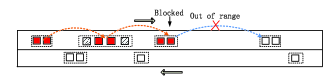
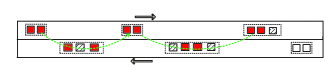
Figure 1: Propagation pattern of a certain packet

II-B Cooperative Transmission Model

Now we will describe the transmission between two clusters, namely a transmitter cluster (TxC) with $N_{t}$ ($N_{t}\geq 2$) vehicles and a receiver cluster (RxC) with $N_{r}$ vehicles. For ease of analysis, only two randomly-chosen vehicles (denoted by filled squares $T_{x1}$ and $T_{x2}$) in TxC are allowed to transmit. The cluster-based transmission model is illustrated in Fig. 2.

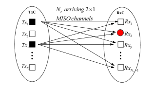
Figure 2: Cluster-based cooperative transmission model

II-B1 Channel Characterization

The virtual MIMO channel between two transmitters and $N_{r}$ receivers can be represented as:

$$\textbf{H}=\left[\textbf{D}_{1}^{\frac{1}{2}}\textbf{s}_{1}\quad\textbf{D}_{2}^{\frac{1}{2}}\textbf{s}_{2}\right]_{N_{r}\times 2},$$ (1)

where $\left[\textbf{s}_{1}\right]_{N_{r}\times 1}$, $\left[\textbf{s}_{2}\right]_{N_{r}\times 1}$ denote the small-scale fading between the RxC and $T_{x1}$ and $T_{x2}$, respectively; $\left[\textbf{D}_{1}^{\frac{1}{2}}\right]_{N_{r}\times N_{r}}$, $\left[\textbf{D}_{2}^{\frac{1}{2}}\right]_{N_{r}\times N_{r}}$ are diagonal matrices accounting for the large scale fading effect. For mathematical tractability, we approximately assume that the large scale fading of each link is almost the same, thus can be defined as $D^{-\delta}$, here $\delta$ is the path loss exponent with typical value from 2 to 4. Furthermore, we assume that the small-scale fading follows Rician distribution, which is typical for a flat terrain. Thus $\left[\textbf{s}_{1}\right]_{N_{r}\times 1}$ and $\left[\textbf{s}_{2}\right]_{N_{r}\times 1}$ can be denoted as follows [rician1]:

$$\textbf{s}_{1}(\theta_{1}) =\sqrt{\frac{K}{K+1}}\textbf{v}(\theta_{1})+\sqrt{\frac{1}{K+1}}\textbf{g}_{1},$$ (2)

$$\textbf{s}_{2}(\theta_{2}) =\sqrt{\frac{K}{K+1}}\textbf{v}(\theta_{2})+\sqrt{\frac{1}{K+1}}\textbf{g}_{2}$$

where $K$ is the Rician factor, $\theta_{1}$ and $\theta_{2}$ are the Angles of Arrivals (AoAs) of signals from $T_{x1}$ and $T_{x2}$, respectively. Note that in our one-dimensional scenario, $\theta_{1}{=}\theta_{2}{=}\theta{=}\pi/2$, thus function $v(\theta)$ is represented as

$$\small v(\theta){=}\left[1,{...}\exp\left({-}jk\frac{2\pi d_{k}}{\lambda}\right),{...},\exp\left({-}j(N_{r}{-}1)\frac{2\pi d_{N_{r}}}{\lambda}\right)\right]^{T},$$ (3)

and $[g_{1}]_{N_{r}\times 1}$, $[g_{2}]_{N_{r}\times 1}\sim{\cal{CN}}(\textbf{0},\textbf{I})$ denote the Rician scattering vector.

II-B2 Opportunistic Retransmission

Given the distributed nature of receivers, we adopt a simplified selection diversity [wireless] algorithm at RxC, over the set of $N_{r}$ MISO channels, i.e., the vehicle with the highest received signal-to-noise ratio (SNR) (denoted by the red-filled circle $R_{x2}$) acts as a coordinator and broadcasts the decoded packet within RxC immediately. We also adopt an ACK-based protocol, so that the coordinator returns a confirmation message (ACK) to TxC on successfully receiving the packet, otherwise the transmitters will keep retransmitting every $\tau$ seconds.

III Transmission Range Gain Analysis

In this section, we will analyze the transmission range gain from the proposed cooperative transmission scheme. Intuitively, power gain, provided by jointly transmitting, together with diversity gain, provided by receiving over independent fading channels, can be leveraged to boost the transmission range.

Assume there exists some minimum receive SNR which can be translated to a minimum received power $P_{min}$ for acceptable performance. Providing the target outage probability $P_{out}$, let $r$ represent the maximal one-hop transmission range of a single vehicle with transmit power $P_{t}$. Based on the flat Rician fading channel model, the received signal on the edge is:

$$y=r^{-\delta/2}\left(\sqrt{\frac{K}{K+1}}+\sqrt{\frac{1}{K+1}}\psi_{0}\right)x+n_{0},$$ (4)

where $\psi_{0}\sim$ $\cal{CN}$ $(0,1)$, and $n_{0}$ denotes the addictive white Gaussian noise with power spectral density $N_{0}$. Apparently,

$$P_{out}=P(P_{0}r^{-\delta}|\psi|^{2}<P_{min}),$$ (5)

where $P_{0}=\frac{KP_{t}}{K{+}1}$ denotes the normalized transmit power and $\psi{=}1{+}\sqrt{\frac{1}{K}}\psi_{0}$.

Lemma 1.

$X$ is an non-central $\chi^{2}$ distributed random variable with $f$ degrees of freedom and non-central parameter $\lambda$, $(\frac{X}{r})^{\frac{1}{3}}$ is approximately normally distributed with mean $1-\frac{2}{9}\frac{1+b}{r}$ and variance $\frac{2}{9}\frac{1+b}{r}$, where $r=f+\lambda$ and $b=\frac{\lambda}{f+\lambda}$.

Proof:

See [ncx].

According to Lemma 1, we get

$$\left(\frac{|\psi|^{2}}{\sigma^{2}\left(2+\frac{1}{\sigma^{2}}\right)}\right)^{\frac{1}{3}}\sim{\cal{N}}\left(M_{1},V_{1}\right),$$ (6)

where $M_{1}=1-\frac{4\sigma^{2}\left(\sigma^{2}+1\right)}{9\left(2\sigma^{2}+1\right)^{2}}$, $V_{1}=\frac{4\sigma^{2}\left(\sigma^{2}+1\right)}{9\left(2\sigma^{2}+1\right)^{2}}$ and $\sigma=\sqrt{\frac{1}{K}}$.

By combining (5) and (6), we easily obtain

$$r=\left[\frac{P_{0}\sigma^{2}\left(2+\frac{1}{\sigma^{2}}\right)\left(\sqrt{V_{1}}\Phi^{-1}\left(P_{out}\right)+M_{1}\right)^{3}}{P_{min}}\right]^{\frac{1}{\delta}}.$$ (7)

In terms of the cooperative scheme, with each vehicle transmitting the same signal with identical transmit power $P_{t}$, the received signal can be represented as:

$$\textbf{y}=\left[\textbf{D}_{1}^{\frac{1}{2}}\textbf{s}_{1}\quad\textbf{D}_{2}^{\frac{1}{2}}\textbf{s}_{2}\right]\left[\begin{array}[]{l}x\\ x\\ \end{array}\right]+\textbf{n},$$ (8)

where $\textbf{E}(x^{2})=P_{t}$ and $[\textbf{n}]_{N_{r}\times 2}\sim{\cal{CN}}(0,\sigma_{N}^{2}\textbf{I})$ is the complex white Gaussian noise vector.

We assume perfect phase compensation at RxC, so the output SNR, based on the selection diversity algorithm, is:

$$\gamma^{SC}=\frac{P_{t}}{N_{0}}\mathop{\max}\limits_{k}|\textbf{h}_{k}|^{2},$$ (9)

where $\textbf{h}_{k}$ denotes the $k$th row of H.

Let $R$ be the expanded transmission range, referred as MIMO range for brevity. Given the same target outage probability on the edge, thus we have

$$P_{out} =P\left(\gamma^{SC}<\frac{P_{min}}{N_{0}}\right)$$ (10)

$$=\prod\limits_{k{=}1}^{N_{r}}{P\left({P_{0}}{R^{-\delta}}\left(|\psi_{k1}|^{2}+|\psi_{k2}|^{2}\right){<}P_{min}\right)}$$

$$=\left[P\left(|\psi_{k1}|^{2}+|\psi_{k2}|^{2}{<}{\frac{P_{min}}{P_{0}R^{-\delta}}}\right)\right]^{N_{r}}$$

Note that the second and the third equality follow from the cumulative density function of the maximum of i.i.d random variables. Similarly, we have $\frac{|\phi_{k1}|^{2}+|\phi_{k2}|^{2}}{\sigma^{2}}\sim\chi^{{}^{\prime}2}_{4}(\frac{2}{\sigma^{2}})$, which gives:

$$R=\left[\frac{2P_{0}\sigma^{2}\left(2+\frac{1}{\sigma^{2}}\right)\left(\sqrt{V_{2}}\Phi^{-1}\left(P_{out}^{\frac{1}{N_{r}}}\right)+M_{2}\right)^{3}}{P_{min}}\right]^{\frac{1}{\delta}},$$ (11)

where $M_{2}=1-\frac{2\sigma^{2}\left(\sigma^{2}+1\right)}{9\left(2\sigma^{2}+1\right)^{2}}$ and $V_{2}=\frac{2\sigma^{2}\left(\sigma^{2}+1\right)}{9\left(2\sigma^{2}+1\right)^{2}}$. By taking the ratio of $R$ and $r$, the transmission range gain is:

$$g=[\frac{2(\sqrt{V_{2}}\Phi^{-1}(P_{out}^{\frac{1}{N_{r}}})+M_{2})^{3}}{(\sqrt{V_{1}}\Phi^{-1}(P_{out})+M_{1})^{3}}]^{\frac{1}{\delta}}.$$ (12)

Since $P_{out}$, $\sigma$ are predetermined constants, $N_{r}$ is left to exclusively affect $g$. Equivalently, we can write $g$ as a function of $N_{r}$:

$$g\buildrel\Delta\over{=}F(N_{r}).$$ (13)

Fig. 3 shows the relationship between $g$ and $N_{r}$, with $N_{r}$ plotted in log-fashion. It can be seen that the range gain grows logarithmically with the number of cooperating vehicles (or cluster size). This implies a few additional cooperating vehicles would be sufficient, and too many cooperators would only incur excessive overhead.

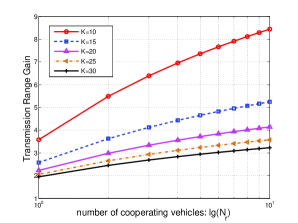
Figure 3: Transmission range gain as number of cooperating vehicles increases

IV Information Propagation Speed Analysis

The technical building blocks for analyzing IPS is organized as follows. IV-A sutdies the distribution of cluster size, i.e., the number of vehicles in a cluster. LABEL:roadlengthgapsub analyzes the average road length ahead until the gap is bridged by the next cluster. In LABEL:unbrigapsub, we investigate the distribution of an unbridged gap length. Based on the results in IV-A to LABEL:unbrigapsub, the expectation of blocking time is obtained in LABEL:subsecT. Meanwhile, the expected distance that a piece of information can propagate after the block is given in LABEL:Dsubsec. Having obtained these key elements, we get the final expression of the IPS in LABEL:IPSsubsec.

IV-A Number of Vehicles Within a Cluster

Lemma 2.

The probability mass function (pmf) of the number of vehicles within a cluster is given by:

$$P_{N}(k)=e^{-\lambda r}(1-e^{-\lambda r})^{k-1}~{}~{}~{}~{}~{}(k=1,2,3\ldots)$$ (14)

and its cumulative distribution function (CDF) of is:

$$F_{N}(n)=P(N\leq n)=1-(1-e^{-\lambda r})^{n},$$ (15)

where $\lambda$ is the poisson intensity.