Heterogeneous Computing on Mixed Unstructured Grids with PyFR

Abstract

PyFR is an open-source high-order accurate computational fluid dynamics solver for mixed unstructured grids that can target a range of hardware platforms from a single codebase. In this paper we demonstrate the ability of PyFR to perform high-order accurate unsteady simulations of flow on mixed unstructured grids using heterogeneous multi-node hardware. Specifically, after benchmarking single-node performance for various platforms, PyFR v0.2.2 is used to undertake simulations of unsteady flow over a circular cylinder at Reynolds number $3\,900$ using a mixed unstructured grid of prismatic and tetrahedral elements on a desktop workstation containing an Intel Xeon E5-2697 v2 CPU, an NVIDIA Tesla K40c GPU, and an AMD FirePro W9100 GPU. Both the performance and accuracy of PyFR are assessed. PyFR v0.2.2 is freely available under a 3-Clause New Style BSD license (see www.pyfr.org).

1 Introduction

There is an increasing desire amongst industrial practitioners of computational fluid dynamics (CFD) to perform scale-resolving simulations of unsteady compressible flows within the vicinity of complex geometries. However, current generation industry-standard CFD software—predominantly based on first- or second-order accurate Reynolds Averaged Navier-Stokes (RANS) technology—is not well suited to the task. Henceforth, over the past decade there has been significant interest in the application of high-order methods for mixed unstructured grids to such problems. Popular examples of high-order schemes for mixed unstructured grids include the discontinuous Galerkin (DG) method, first introduced by Reed and Hill [1], and the spectral difference (SD) methods originally proposed under the moniker ‘staggered-gird Chebyshev multidomain methods’ by Kopriva and Kolias in 1996 [2] and later popularised by Sun et al. [3]. In 2007 Huynh [4] proposed the flux reconstruction (FR) approach; a unifying framework for high-order schemes on unstructured grids that incorporates both the nodal DG schemes of [5] and, at least for a linear flux function, any SD scheme. In addition to offering high-order accuracy on unstructured mixed grids, FR schemes are also compact in space, and thus when combined with explicit time marching offer a significant degree of element locality. This locality makes such schemes extremely good candidates for acceleration using either the vector units of modern CPUs or graphics processing units (GPUs) [6, 7, 8]. There exist a variety of approaches for writing accelerated codes. These include directive based methodologies such as OpenMP 4.0 and OpenACC, and language frameworks such as OpenCL and CUDA. Unfortunately, at the time of writing, there exists no single approach which is performance portable across all major hardware platforms. Codes desiring cross-platform portability must therefore incorporate support for multiple approaches. Further, there is also a growing interest from the scientific community in heterogeneous computing whereby multiple platforms are employed simultaneously to solve a problem. The promise of heterogeneous computing is improved resource utilisation on systems with a mix of hardware. Such systems are becoming increasingly common.

PyFR is a high-order FR code for solving the Euler and compressible Navier-Stokes equations on mixed unstructured grids [8]. Written in the Python programming language PyFR incorporates backends for C/OpenMP, CUDA, and OpenCL. It is therefore capable of running on conventional CPUs, as well as GPUs from both NVIDIA and AMD, as well as heterogeneous mixtures of the aforementioned. The objective of this paper is to demonstrate the ability of PyFR to perform high-order accurate unsteady simulations of flow on mixed unstructured meshes using a heterogeneous hardware platform—demonstrating the concept of ‘heterogeneous computing from a homogeneous codebase’. Specifically, we will undertake simulations of unsteady flow over a cylinder at Reynolds number $3\,900$ using a mixed unstructured grid of prismatic and tetrahedral elements using a desktop workstation containing an Intel Xeon E5-2697 v2 CPU, an NVIDIA Tesla K40c GPU, and an AMD FirePro W9100 GPU. At the time of writing these represent the high-end workstation offerings from the three major hardware vendors. All are designed for workstations with support for error-correcting code (ECC) memory and double precision floating point arithmetic.

The paper is structured as follows. In section 2 we provide a brief overview of the PyFR codebase. In section section 3 we provide details of the cylinder test case. In section 4 single node performance is discussed. In section 5 multi-node heterogeneous performance is discussed, and finally in section 6 conclusions are drawn.

2 PyFR

2.1 Overview

For a detailed overview of PyFR the reader is referred to Witherden et al. [8]. Key functionality of PyFR v0.2.2 is summarised in Table 1. We note that PyFR achieves platform portability via use of an innovative ‘backend’ infrastructure.

Table 1: Key functionality of PyFR v0.2.2.

Dimensions	2D, 3D
Elements	Triangles, Quadrilaterals, Hexahedra,
	Tetrahedra, Prisms
Spatial orders	Arbitrary
Time steppers	Euler, RK4, RK45
Precisions	Single, Double
Platforms	CPUs, NVIDIA GPUs, AMD GPUs
Inter-Node Communication	MPI
Governing Systems	Euler, Compressible Navier-Stokes

The majority of operations within an FR time-step can be cast as matrix multiplications of the form

$$\bm{\mathsf{C}}\leftarrow c_{1}\bm{\mathsf{A}}\bm{\mathsf{B}}+c_{2}\bm{\mathsf{C}},$$ (1)

where $c_{1,2}\in\mathbb{R}$ are scalar constants, $\bm{\mathsf{A}}$ is a constant operator matrix, and $\bm{\mathsf{B}}$ and $\bm{\mathsf{C}}$ are row-major state matrices. Within the taxonomy proposed by Goto et al. [9] the multiplications fall into the block-by-panel (GEBP) category. The specific dimensions of the operator matrices are a function of both the polynomial order $\wp$ used to represent the solution in each element of the domain, and the element type. A breakdown of these dimensions for the volume-to-surface interpolation operator matrix $\bm{\mathsf{M}}^{0}$ can be found in Table 2. In PyFR platform portability of the matrix multiply operations is achieved by deferring to the GEMM family of subroutines provided by a Basic Linear Algebra Subprograms (BLAS) library for the target platform.

Table 2: Dimensions of the volume-to-surface interpolation operator matrix $\bm{\mathsf{M}}^{0}$ at orders $\wp=1,2,3,4$ for tetrahedral, prismatic, and hexahedral element types.

	$\dim{\bm{\mathsf{M}}^{0}}$
Type	$\wp=1$	$\wp=2$	$\wp=3$	$\wp=4$
Tet	$4\times 12$	$10\times 24$	$20\times 40$	$\hphantom{0}35\times 60$
Pri	$6\times 18$	$18\times 39$	$40\times 68$	$\hphantom{0}75\times 105$
Hex	$8\times 24$	$27\times 54$	$64\times 96$	$125\times 150$

All other operations involved in an FR time-step are point-wise, concerning themselves solely with data at an individual solution/flux point. In PyFR platform portability of these point-wise operations is achieved via use of a bespoke domain specific language based on the Mako templating engine [10]. Mako specifications of point-wise operations are converted into backend-specific low-level code for the target platform at runtime, which is then compiled, linked and loaded into PyFR.

2.2 C/OpenMP backend

The C/OpenMP backend can be used to target CPUs from a range of vendors. The BLAS implementation employed by PyFR for the C/OpenMP backend must be specified by the user at runtime. Both single- and multi-threaded libraries are supported. When a single-threaded library is specified PyFR will perform its own parallelisation. Given a state matrix $\bm{\mathsf{B}}$ of dimension $(K,N)$ the decomposition algorithm splits $\bm{\mathsf{B}}$ into $N_{t}$ slices of dimension $(K,N/N_{t})$ where $N_{t}$ is the number of OpenMP threads. Each thread then multiplies its slice through by $\bm{\mathsf{A}}$ to yield the corresponding slice of $\bm{\mathsf{C}}$. A visualisation of this approach is shown in Figure 1. For the block-by-panel multiplications encountered in FR this strategy has been found to consistently outperform those employed by multi-threaded BLAS libraries.

$$\underbrace{\left[\vphantom{\int}\;\;\hphantom{\ldots}\;\;\middle|\;\;\hphantom{\ldots}\;\;\middle|\;\;\ldots\;\;\middle|\;\;\hphantom{\ldots}\;\;\middle|\;\;\hphantom{\ldots}\;\;\right]}_{\bm{\mathsf{C}}}=\underbrace{\left[\vphantom{\int}\;\;\hphantom{\ldots}\;\;\right]}_{\bm{\mathsf{A}}}\underbrace{\left[\vphantom{\int}\;\;\hphantom{\ldots}\;\;\middle|\;\;\hphantom{\ldots}\;\;\middle|\;\;\ldots\;\;\middle|\;\;\hphantom{\ldots}\;\;\middle|\;\;\hphantom{\ldots}\;\;\right]}_{\bm{\mathsf{B}}}$$

Figure 1: How matrix multiplications are parallelised in the C/OpenMP backend of PyFR.

2.3 CUDA backend

The CUDA backend can be used to target NVIDIA GPUs of compute capability 2.0 or later. PyCUDA [11] is used to invoke the CUDA API from Python. Matrix-multiplications are performed using the cuBLAS library which ships as part of the CUDA distribution. The cuBLAS library is exclusively column-major. Nevertheless it is possible to directly multiply two row-major matrices together by utilising the fact that

$$\bm{\mathsf{C}}=\bm{\mathsf{A}}\bm{\mathsf{B}}\implies\bm{\mathsf{C}}^{T}=(\bm{\mathsf{A}}\bm{\mathsf{B}})^{T}=\bm{\mathsf{B}}^{T}\bm{\mathsf{A}}^{T},$$ (2)

and observing the effect of passing a row-major matrix to a column-major subroutine is to implicitly transpose it.

2.4 OpenCL backend

The OpenCL backend can be used to target CPUs and GPUs from a range of vendors. The PyOpenCL package [11] is used to interface OpenCL with Python. OpenCL natively supports runtime code generation. BLAS support is provided via the open source clBLAS library, which is primarily developed and supported by AMD. For GPU devices clBLAS utilises auto-tuning in order to effectively target a wide range of architectures. Performance is heavily dependent on the underlying OpenCL implementation.

2.5 Distributed memory systems

To scale out across multiple nodes PyFR utilises the Message Passing Interface (MPI). By construction the data exchanged between MPI ranks is independent of the backend being used. A natural consequence of this is that different MPI ranks can transparently utilise different backends—hence enabling PyFR to run on heterogenous multi-node systems.

3 Cylinder Test Case

3.1 Overview

Flow over a circular cylinder has been the focus of numerous previous experimental and numerical studies. Characteristics of the flow are known to be highly dependent on the Reynolds number $Re$, defined as

$$Re=\frac{u_{\infty}D}{\nu},$$ (3)

where $u_{\infty}$ is the free-stream fluid speed, $D$ is the cylinder diameter, and $\nu$ is the fluid kinematic viscosity. Roshko [12] identified a stable range between $Re=40$ and $150$ that is characterised by the shedding of regular laminar vortices, as well as a transitional range between $Re=150$ and $300$, and a turbulent range beyond $Re=300$. These results were subsequently confirmed by Bloor [13], who identified a similar set of regimes. Later, Williamson [14] identified two modes of transition from two dimensional to three dimensional flow. The first, known as Mode-A instability, occurs at $Re\approx 190$ and the second, known as Mode-B instability, occurs at $Re\approx 260$. The turbulent range beyond $Re=300$ can be further sub-classified into the shear-layer transition, critical, and supercritical regimes as discussed in the review by Williamson [15].

In the present study we consider flow over a circular cylinder at $Re=3\,900$, and an effectively incompressible Mach number of $0.2$. This case sits in the shear-layer transition regime identified by Williamson [15], and contains several complex flow features, including separated shear layers, turbulent transition, and a fully turbulent wake.

3.2 Domain

In the present study we use a computational domain with dimensions $[-9D,25D]$; $[-9D,9D]$; and $[0,\pi D]$ in the stream-, cross-, and span-wise directions, respectively. The cylinder is centred at $(0,0,0)$. The span-wise extent was chosen based on the results of Norberg [18], who found no significant influence on statistical data when the span-wise dimension was doubled from $\pi D$ to $2\pi D$. Indeed, a span of $\pi D$ has been used in the majority of previous numerical studies [16, 19, 20], including the recent DNS study of Lehmkuhl et al. [21]. The stream-wise and cross-wise dimensions are comparable to the experimental and numerical values used by Parnaudeau et al. [22], whose results will be directly compared with ours. The overall domain dimensions are also comparable to those used for DNS studies by Lehmkuhl et al. [21]. The domain is periodic in the span-wise direction, with a no-slip isothermal wall boundary condition applied at the surface of the cylinder, and Riemann invariant boundary conditions applied at the far-field.

3.3 Mesh

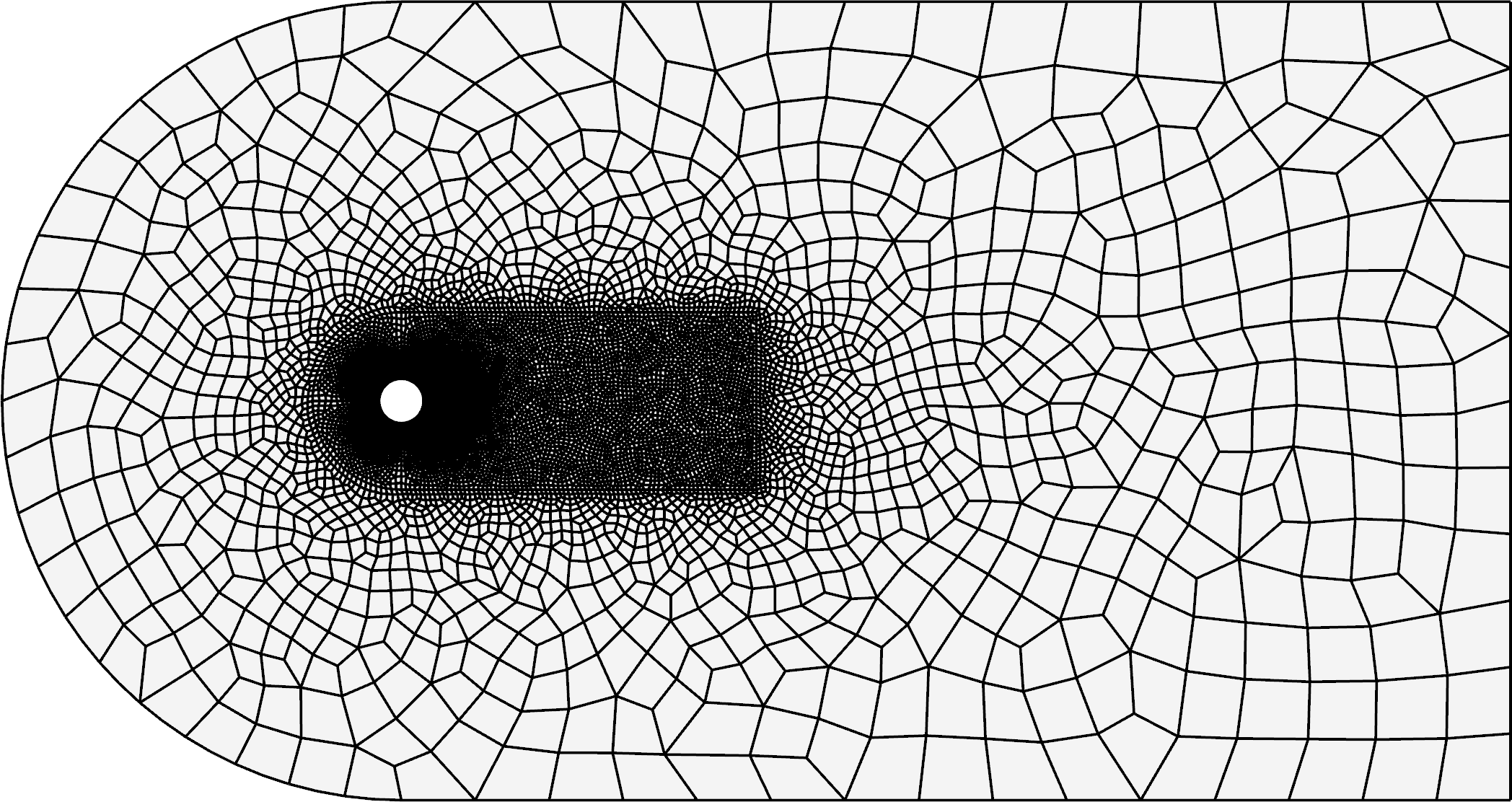
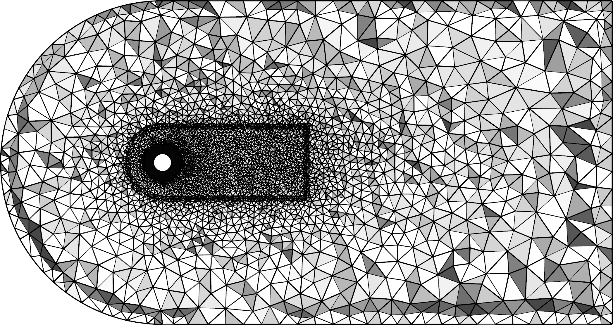
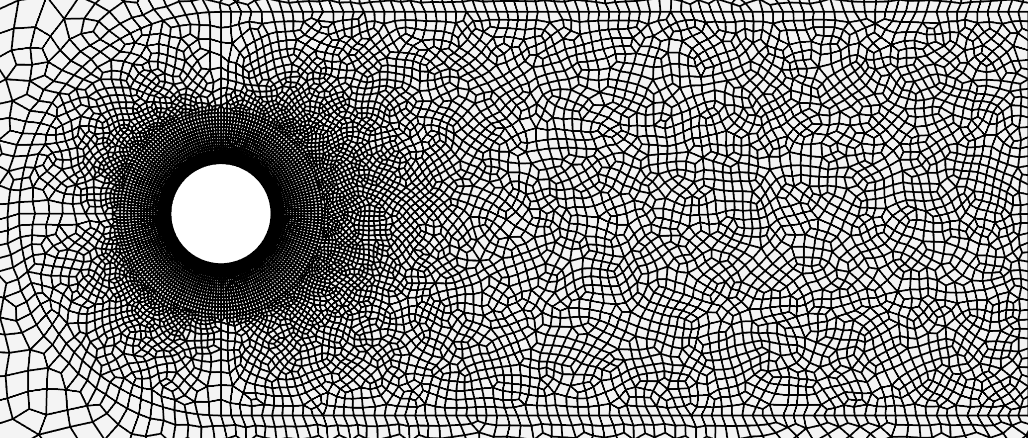
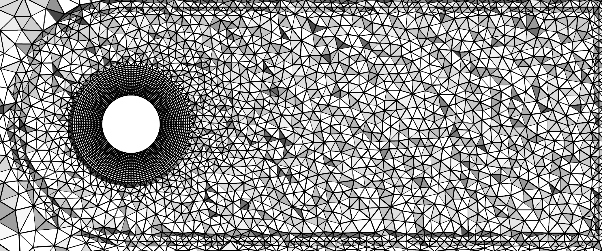
The domain was meshed in two ways. The first mesh consisted of entirely hexahedral elements, and the second a mixture of prismatic elements in the near wall boundary layer region, and tetrahedral elements in the wake and far-field. Both meshes employed quadratically curved elements, and were designed to fully resolve the near wall boundary layer region when $\wp=4$. Specifically, the maximum skin friction coefficient was estimated a priori as $C_{f}\approx 0.075$ based on the LES results of Breuer [19]. The height of the first element was then specified such that when $\wp=4$ the first solution point from the wall sits at $y+\approx 1$, where non-dimensional wall units are calculated in the usual fashion as $y+=u_{\tau}y/\nu$ with $u_{\tau}=\sqrt{C_{f}/2}u_{\infty}$.

The hexahedral mesh had 200 elements in the circumferential direction, and 10 elements in the span-wise direction, which when $\wp=4$ achieves span-wise resolution comparable to that used in previous studies; as discussed by Breuer [19] and the references contained therein. The prism/tetrahedral mesh has 120 elements in the circumferential direction, and 20 elements in the span-wise direction, these numbers being chosen to help reduce face aspect ratios at the edges of the prismatic layer; which facilitates transition to the fully unstructured tetrahedral elements in the far-field. In total the hexahedral mesh contained $118\,070$ elements, and the prism/tetrahedral mesh contained $79\,344$ prismatic elements and $227\,298$ tetrahedral elements. Both meshes are shown in Figure 2.

(a) Hexahedral, far-field.

(b) Prism/tetrahedral, far-field.

(c) Hexahedral, wake.

(d) Prism/tetrahedral, wake.

Figure 2: Cutaways through the two meshes.

3.4 Methodology

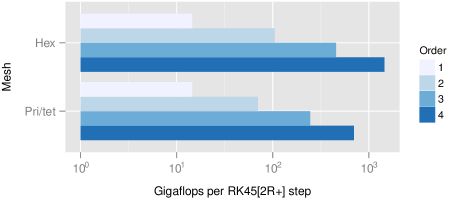
The compressible Navier-Stokes equations, with constant viscosity, were solved on each of the two meshes shown in Figure 2. A DG scheme was used for the spatial discretisation, a Rusanov Riemann solver was used to calculate the inviscid fluxes at element interfaces, and the explicit RK45[2R+] scheme of Carpenter and Kennedy [23] was used to advance the solution in time. No sub-grid model was employed, hence the approach should be considered ILES/DNS, as opposed to classical LES. Values of $\wp$ from one to four were used with each mesh. The approximate memory requirements of PyFR for these simulations can are detailed in Table 3. The total number of floating point operations required by an RK45[2R+] time-step for each simulation are detailed in Figure 3. When running with $\wp=1$ both meshes require ${\sim}1.5\times 10^{10}$ floating point operations per time-step. This number can be seen to increase rapidly with the polynomial order.

Table 3: Approximate memory requirements of PyFR for the two cylinder meshes.

	Device memory / GiB
Mesh	$\wp=1$	$\wp=2$	$\wp=3$	$\wp=4$
Hex	$0.8$	$2.0$	$4.1$	$7.2$
Pri/tet	$1.1$	$2.6$	$4.7$	$7.7$

Figure 3: Computational effort required for the $118\,070$ element hexahedral mesh and the mixed mesh with $79\,344$ prismatic elements and $227\,298$ tetrahedral elements.

4 Single-Node Performance

4.1 Overview

In this section we will analyse performance of PyFR on an Intel Xeon E5-2697 v2 CPU, an NVIDIA Tesla K40c GPU, and an AMD FirePro W9100 GPU. These are the individual platforms used to construct the multi-node heterogeneous system employed in section 5.

4.2 Hardware specifications

Various attributes of the E5-2697, K40c, and W9100 are detailed in Table 4. The theoretical peaks for double precision arithmetic and memory bandwidth were obtained from vendor specifications. However, in practice it is usually only possible to obtain these theoretical peak values using specially crafted code sequences. Such sequences are almost always platform specific and seldom perform useful computations. Consequently, we also calculate and tabulate reference peaks. Reference peaks for double precision arithmetic are defined here as the maximum number of giga floating point operations per second (GFLOP/s) obtained while multiplying two large double precision row-major matrices using DGEMM from an appropriate BLAS library. Reference peaks for memory bandwidth are defined here as the rate, in gigabytes per second (GB/s), that data can be copied between two one gigabyte buffers. Reference peaks for the E5-2697 were obtained using DGEMM from the Intel Math Kernel Libraries (MKL) version 11.1.2, and with the E5-2697 paired with four DDR3-1600 DIMMs (with Turbo Boost enabled). Reference peaks for the K40c were obtained using DGEMM from cuBLAS as shipped with CUDA 6, with GPU boost disabled and ECC enabled. Reference peaks for the W9100 were obtained using DGEMM from clBLAS v2.0 with version 1411.4 of the AMD APP OpenCL runtime. ECC settings for the W9100 were left unchanged.

We note that on the K40c ECC is implemented in software, and when enabled error-correction data is stored in global memory. A consequence of this is that when ECC is enabled there is a reduction in available memory and memory bandwidth. This partially accounts for the discrepancy observed between the theoretical and reference memory bandwidths for the K40c. We also note that for the K40c and the E5-2697, reference peaks for double precision arithmetic are in excess of 80% of their theoretical values. However, for the W9100 the reference peak for double precision arithmetic is only 34% of its theoretical value. This value is not significantly improved via the auto-tuning utility that ships with clBLAS. It is hoped that this figure will improve with future releases of clBLAS.

Table 4: Baseline attributes of the three hardware platforms. For the NVIDIA Tesla K40c GPU Boost was left disabled and ECC was enabled. The Intel Xeon E5-2697 v2 was paired with four DDR3-1600 DIMMs with Turbo Boost enabled.

	Platform
	K40c	W9100	E5-2697
Arithmetic / GFLOP/s
theoretical peak	1430	2620	280
reference peak	1192	890	231
Memory Bandwidth / GB/s
theoretical peak	288	320	51.2
reference peak	190	261	37.1
Thermal Design Power / W	235	275	130
Memory / GB	12	16
Clock / MHz	745	930	3000
Transistors / Billion	7.1	6.2	4.3

Finally, as an aside, we note that the number of ‘cores’ available on each platform have been deliberately omitted from Table 4. It is our contention that the term is both ill-defined and routinely subject to abuse in the literature. For example, the E5-2697 is presented by Intel as having 12 cores, whereas the K40c is described by NVIDIA as having 2880 ‘CUDA cores’. However, whereas the cores in the E5-2697 can be considered linearly independent those in the K40c can not. The rough equivalent of a CPU core in NVIDIA parlance is a ‘streaming multiprocessor’, or SMX, of which the K40c has 15. Additionally, the E5-2697 has support for two-way simultaneous multithreading—referred to by Intel as Hyper-Threading—permitting two threads to execute on each core. At any one instant it is therefore possible to have up to 24 independent threads resident on a single E5-2697. The AMD equivalent of a CUDA core is a ‘stream processor’ of which the W9100 has 2816. This is not to be confused with the aforementioned streaming multiprocessor of NVIDIA; for which the AMD equivalent is a ‘Compute Unit’. Practically, both CUDA cores and stream processors are closer to the individual vector lanes of a traditional CPU core. Given this minefield of confusing nomenclature we have instead opted to simply state the peak floating point capabilities of the hardware.

4.3 Performance

By measuring the wall clock time required for PyFR to take a defined number of time-steps, and utilising the operation counts per time-step detailed in Figure 3, one can calculated the sustained performance of PyFR in GFLOP/s when running with the meshes detailed in subsection 3.3 and $\wp=1,2,3,4$.

Sustained performance of PyFR for the various hardware platforms is shown in Figure 4. From the figure it is clear that the computational efficiency of PyFR increases with the polynomial order. This is consistent with higher order simulations having an increased compute intensity per degree of freedom. This additional intensity results in larger operator matrices that are better suited to the tiling schemes employed by BLAS libraries. The OpenCL implementation shipped by NVIDIA as part of CUDA only supports the use of 32-bit memory pointers. As such a single context is limited to $4\,\text{GiB}$ of memory, cf. Table 3. It was therefore not possible to perform the third and fourth order simulations for either of the two meshes using the OpenCL backend with the K40c.

Figure 4: Sustained performance of PyFR in GFLOP/s for the various pieces of hardware. The backend used by PyFR is given in parentheses. For the OpenCL backend the initial of the vendor is suffixed. As the NVIDIA OpenCL platform is limited to $4\,\text{GiB}$ of memory no results are available for $\wp=3,4$.

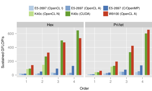
The Intel and AMD implementations of OpenCL, when used in conjunction with clBLAS, are only competitive with the C/OpenMP backend when $\wp=1$ for the hexahedral mesh, and $\wp=1,2$ for the prism/tetrahedral mesh. This is also the case when comparing performance between the CUDA backend and the NVIDIA OpenCL backend on the K40c. Prior analysis by Witherden et al. [8] suggests that at these orders a reasonable proportion of the wall clock time will be spent in the bandwidth-bound point-wise kernels as opposed to DGEMM. On account of being bandwidth-bound such kernels do not extensively test the optimisation capabilities of the compiler. By the time $\wp=4$ both implementations of OpenCL on the E5-2697 are delivering between one third and one quarter of the performance of the native backends. This highlights the difficulties associated with writing a performant DGEMM routine and hence severely impacts the performance portability of the OpenCL backend. This result lends credence to our opening assertion that there are currently no programming methodologies that are performance portable across a range of platforms. Further, it also justifies the approach that has been adopted by PyFR.

Performance of the K40c culminates at $647\,\text{GFLOP/s}$ for the $\wp=4$ hexahedral mesh. This represents some $45\%$ of the theoretical peak and $54\%$ of the reference peak. By comparison the E5-2697 obtains $132\,\text{GFLOP/s}$ for the same simulation equating to $47\%$ and $57\%$ of the theoretical and reference peaks, respectively. Performance does improve slightly to $140\,\text{GFLOP/s}$ for the $\wp=4$ prism/tetrahedral mesh, however. On this same mesh at $\wp=4$ the W9100 can be seen to sustain $657\,\text{GFLOP/s}$ of throughput. Although, in absolute terms, this observation represents the highest sustained rate of throughput it corresponds to just $25\%$ of the theoretical peak. However, working in terms of realisable peaks, we find PyFR obtaining some $74\%$ of the reference value.

5 Multi-Node Heterogeneous Performance and Accuracy

5.1 Overview

Having determined the performance characteristics of PyFR on various individual platforms, we will now investigate the ability of PyFR to undertake simulations on a multi-node heterogeneous system containing an Intel Xeon E5-2697 v2 CPU, an NVIDIA Tesla K40c GPU, and an AMD FirePro W9100 GPU.

5.2 Mesh partitioning

In order to distribute a simulation across the nodes of the heterogeneous system it is first necessary to partition the mesh. High quality partitions can be readily obtained using a graph partitioning package such as METIS [24] or SCOTCH [25].

When partitioning a mixed element mesh for a homogeneous cluster it is necessary to suitably weight each element type according to its computational cost. This cost depends both upon the platform on which PyFR is running and the order at which the simulation is being performed. In principle it is possible to measure this cost; however in practice the following set of weights have been found to give satisfactory results across most polynomial orders and platforms

$$\text{hex}:\text{pri}:\text{tet}=3:2:1,$$

where larger numbers indicate a greater computational cost. One subtlety that arises here, is that from a graph partitioning standpoint there is no penalty associated with placing a sole vertex (element) of a given weight inside of a partition. Computationally, however, there is a very real penalty incurred from having just a single element of a certain type inside of the partition. It is therefore desirable to avoid mesh partitions where any one partition contains less than around a thousand elements of a given type. An exception is when a partition contains no elements of such a type—in which case zero overheads are incurred.

When partitioning a mesh with one type of element for a heterogeneous cluster it is necessary to weight the partition sizes in line with the performance characteristics of the hardware on each node. However, in the case of a mixed element mesh on a heterogeneous cluster the weight of an element is no longer static but rather depends on the partition that it is placed in—a significantly richer problem. Solving such a problem is currently beyond the capabilities of most graph partitioning packages. Accordingly, mixed element meshes that are partitioned for heterogeneous clusters often exhibit inferior load balancing than those partitioned for homogeneous systems. Moreover, for consistent performance it is necessary to dedicate a CPU core to each accelerator in the system. The amount of useful computation that can be performed by the host CPU is therefore reduced in accordance with this.

Given the single-node performance numbers of Figure 4 it comports to pair the E5-2697 with the C/OpenMP backend, the K40c with the CUDA backend, and the W9100 with the OpenCL backend, in order to achieve optimal performance. Employing the results of Figure 4, in conjunction with some light experimentation, a set of partitioning weights were obtained and are tabulated in Table 5.

Table 5: Partition weights for the multi-node heterogeneous simulation.

	$\text{E5-2697}:\text{W9100}:\text{K40c}$
Mesh	$\wp=1$	$\wp=2$	$\wp=3$	$\wp=4$
Hex	$3{:}27{:}23$	$3{:}27{:}24$	$4{:}24{:}26$	$4{:}24{:}28$
Pri/tet	$5{:}33{:}17$	$5{:}33{:}17$	$5{:}30{:}20$	$5{:}27{:}23$

5.3 Performance

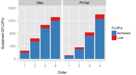
Sustained performance of PyFR on the multi-node heterogeneous system for each of the meshes detailed in subsection 3.3 with $\wp=1,2,3,4$ is shown in Figure 5. Under the assumptions of perfect partitioning and scaling one would expect the sustained performance of the heterogeneous simulation to be equivalent to the sum of the E5-2697 (C/OpenMP), K40c (CUDA), and W9100 (OpenCL A) bars in Figure 4. However, for reasons outlined in the preceding paragraphs these assumptions are unlikely to hold. Some of the available FLOP/s can therefore be considered as ‘lost’. For the hexahedral mesh the fraction of lost FLOP/s varies from $22.5\%$ when $\wp=1$ to $8.7\%$ in the case of $\wp=4$. With the exception of $\wp=1$ the fraction of lost FLOP/s are a few percent higher for the mixed mesh. This is understandable given the additional complexities associated with mixed mesh partitioning and can likely be improved upon by switching to order-dependent element weighting factors.

Figure 5: Sustained performance of PyFR on the multi-node heterogeneous system for each mesh with $\wp=1,2,3,4$. Lost FLOP/s represent the difference between the achieved FLOP/s and the sum of the E5-2697 (C/OpenMP), K40c (CUDA), and W9100 (OpenCL A) bars in Figure 4.

5.4 Accuracy

In this section we present instantaneous and time-span-averaged (henceforth referred to as averaged) results obtained using the multi-node heterogeneous system and the mixed unstructured prism/tetrahedral mesh with $\wp=1,2,3,4$. Following the approach of Breuer [19] all averaged results were obtained over $100D/u_{\infty}$ in time, and the full span of the domain. The $\wp=1$ simulation was initialised with spatially constant free-stream initial conditions, and run for a lead in time of ${\sim}50D/u_{\infty}$ before time-averaging began. Subsequent simulations, at $\wp>1$, were initialised with the final solution state from the previous simulation at $\wp-1$, and time-averaging began immediately. For all $\wp$ this approach led to averaged results exhibiting U-shape or Mode-L characteristics (following the terminology of Ma et al. [16] and Lehmkuhl et al. [21] respectively). Hence, all averaged results were compared with the experimental results of Norberg et al. [18] and Parnaudeau et al. [17], which also exhibited U-shape/Mode-L characteristics, as well as Mode-L results from the recent DNS study of Lehmkuhl et al. [21].

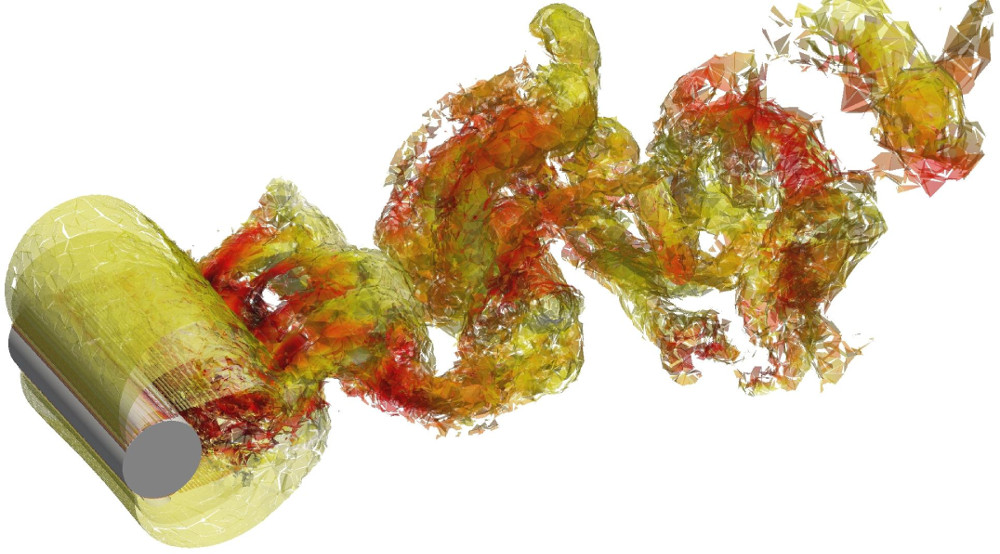
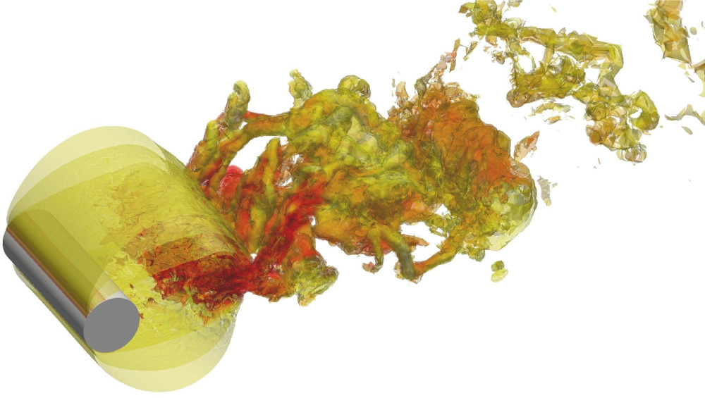
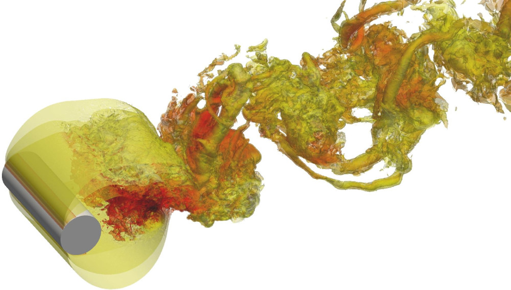
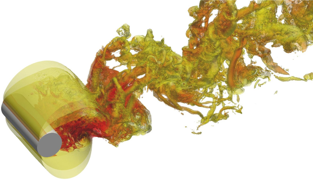
Instantaneous surfaces of iso-density are shown in Figure 6 for each polynomial order. We observe that the $\wp=1$ simulation captures predominantly large-scale structures in the turbulent wake behind the cylinder. As $\wp$ is increased we are able to capture a greater number of small scale turbulent structures. This is due to an increase in the total number of degrees of freedom in the domain, as well as a relative decrease in discretisation errors for the higher-order schemes. We observe laminar flow at the leading edge of the cylinder for all test cases, transition near the separation points, and finally turbulent flow in the wake region. These are the characteristic features of the shear-layer transition regime as described by Williamson [15].

(a) $\wp=1$.

(b) $\wp=2$.

(c) $\wp=3$.

(d) $\wp=4$.

Figure 6: Instantaneous surfaces of iso-density coloured by velocity magnitude.

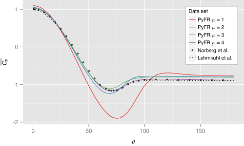
Plots of averaged pressure coefficient $\overline{C_{p}}$ on the surface of the cylinder are shown in Figure 7. The results are shown alongside the experimental results of Norberg et al. [18] (extracted from Kravchenko and Moin [20]), and the Mode-L DNS results of Lehmkuhl et al. [21]. At $\wp=1$ we observe a large negative pressure coefficient near the top and bottom of the cylinder, which includes the location of maximum skin friction coefficient [19]. However, with increasing $\wp$ the results tend towards those of the previous studies.

The averaged pressure coefficient at the base of the cylinder $\overline{C_{pb}}$, and the averaged separation angle $\theta_{s}$ measured from the leading stagnation point are tabulated in Table 6, along with experimental data from Norberg et al. [18] at a similar $Re=4020$ (extracted from Kravchenko and Moin [20]), experimental data from Parnaudeau et al. [17], and Mode-L DNS data from Lehmkuhl et al. [21]. Once again, with increasing $\wp$ the results tend towards those of the previous studies.

Figure 7: Averaged pressure coefficient for $\wp=1,2,3,4$ compared with the experimental results of Norberg et al. [18] (from Kravchenko and Moin [20]) and DNS results of Lehmkuhl et al. [21].

Table 6: Comparison of quantitative values with experimental and DNS results.

	$-\overline{C_{pb}}$	$\theta_{s}/{}^{\circ}$
PyFR pri/tet $\wp=1$	$0.752$	$92$
PyFR pri/tet $\wp=2$	$0.796$	$89$
PyFR pri/tet $\wp=3$	$0.808$	$88$
PyFR pri/tet $\wp=4$	$0.881$	$88$
Parnaudeau et al. [17]		$88$
Lehmkuhl et al. [21]	$0.877$	$87.8$
Norberg et al. [18, 20]	$0.880$

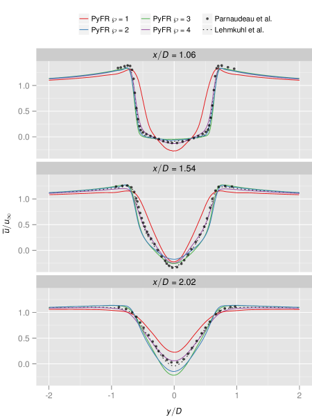
Plots of averaged stream-wise velocity at $x/D=1.06$, $1.54$, and $2.02$ are shown in Figure 8. The results are shown alongside the experimental results of Parnaudeau et al. [17] and the Mode-L DNS results of Lehmkuhl et al. [21]. With $\wp=1$ the profiles deviate significantly from the previous studies. On increasing the order to $\wp=2$ the results are improved. We observe a U-shape profile at $x/D=1.06$, with strong gradients near the mixing layer between the wake and the free stream. The $\wp=4$ results agree well those of the previous studies. The only exception is the reduced magnitude of the averaged velocity deficit near the centre of the wake at $x/D=1.54$.

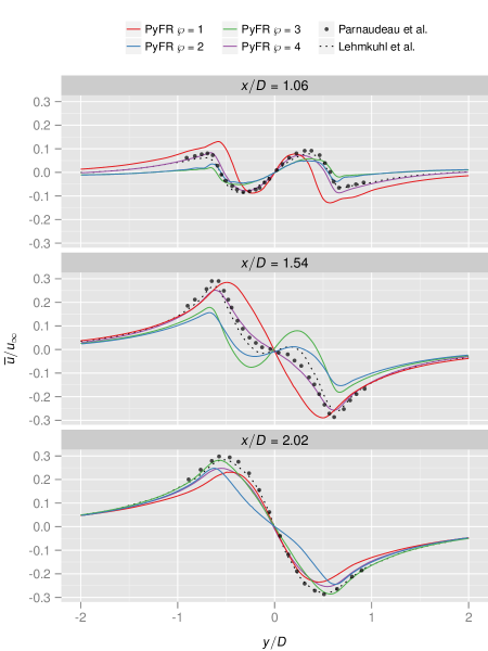
Plots of averaged cross-wise velocity at $x/D=1.06$, $1.54$, and $2.02$ are shown in Figure 9. The results are also shown alongside the experimental results of Parnaudeau et al. [17] and the Mode-L DNS results of Lehmkuhl et al. [21]. The $\wp=4$ results agree well with those of the previous studies.

Figure 8: Time-span-average stream-wise velocity for $\wp=1,2,3,4$ compared with the experimental results of Parnaudeau et al. [17] and DNS results of Lehmkuhl et al. [21].

Figure 9: Time-span-average cross-stream velocity for $\wp=1,2,3,4$ compared with the experimental results of Parnaudeau et al. [17] and DNS results of Lehmkuhl et al. [21].

6 Conclusions

In this paper we have demonstrated the ability of PyFR to perform high-order accurate unsteady simulations of flow on mixed unstructured grids using heterogeneous multi-node hardware. Specifically, after benchmarking single-node performance for various platforms, PyFR v0.2.2 was used to undertake simulations of unsteady flow over a circular cylinder at Reynolds number $3\,900$ using a mixed unstructured grid of prismatic and tetrahedral elements on a desktop workstation containing an Intel Xeon E5-2697 v2 CPU, an NVIDIA Tesla K40c GPU, and an AMD FirePro W9100 GPU. Results demonstrate that PyFR achieves performance portability across various hardware platforms. In particular, the ability of PyFR to target individual platforms with their ‘native’ language leads to significantly enhanced performance cf. targeting each platform with OpenCL alone. PyFR was also found to be performant on the heterogeneous multi-node system achieving a significant fraction of the available FLOP/s. Further, the numerical results obtained using a mixed unstructured grid of prismatic and tetrahedral elements were found to be in good agreement with previous experimental and numerical data.

References

- [1] WH Reed and TR Hill. Triangular mesh methods for the neutron transport equation. Technical Report LA-UR-73-479, Los Alamos Scientific Laboratory, 1973.
- [2] David A Kopriva and John H Kolias. A conservative staggered-grid Chebyshev multidomain method for compressible flows. Journal of computational physics, 125(1):244–261, 1996.
- [3] Yuzhi Sun, Zhi Jian Wang, and Yen Liu. High-order multidomain spectral difference method for the Navier-Stokes equations on unstructured hexahedral grids. Communications in Computational Physics, 2(2):310–333, 2007.
- [4] HT Huynh. A flux reconstruction approach to high-order schemes including discontinuous Galerkin methods. AIAA paper, 4079:2007, 2007.
- [5] Jan S Hesthaven and Tim Warburton. Nodal discontinuous Galerkin methods: algorithms, analysis, and applications, volume 54. Springer Verlag New York, 2008.
- [6] Andreas Klöckner, Tim Warburton, Jeff Bridge, and Jan S Hesthaven. Nodal discontinuous Galerkin methods on graphics processors. Journal of Computational Physics, 228(21):7863–7882, 2009.
- [7] Patrice Castonguay, David M Williams, Peter E Vincent, Manuel Lopez, and Antony Jameson. On the development of a high-order, multi-gpu enabled, compressible viscous flow solver for mixed unstructured grids. AIAA paper, 3229:2011, 2011.
- [8] F.D. Witherden, A.M. Farrington, and P.E. Vincent. PyFR: An open source framework for solving advection–diffusion type problems on streaming architectures using the flux reconstruction approach. Computer Physics Communications, 185(11):3028–3040, 2014.
- [9] Kazushige Goto and Robert A Geijn. Anatomy of high-performance matrix multiplication. ACM Transactions on Mathematical Software (TOMS), 34(3):12, 2008.
- [10] Michael Bayer. Mako: Templates for python, 2013.
- [11] Andreas Klöckner, Nicolas Pinto, Yunsup Lee, Bryan Catanzaro, Paul Ivanov, and Ahmed Fasih. Pycuda and pyopencl: A scripting-based approach to gpu run-time code generation. Parallel Comput., 38(3):157–174, 2012.
- [12] Anatol Roshko. On the development of turbulent wakes from vortex streets. Technical Report No. NACA TR 1191, California Institute of Technology, 1953.
- [13] MS Bloor. The transition to turbulence in the wake of a circular cylinder. Journal of Fluid Mechanics, 19:290–304, 1964.
- [14] CHK Williamson. The existence of two stages in the transition to three dimensionality of a cylinder wake. Physics of Fluids, 31:3165–3168, 1988.
- [15] CHK Williamson. Vortex dynamics in the cylinder wake. Annual Review of Fluid Mechanics, 28:477–539, 1996.
- [16] X Ma, GS Karamanos, and GE Karniadakis. Dynamics and low-dimensionality of a turbulent near wake. Journal of Fluid Mechanics, 310:29–65, 2000.
- [17] P Parnaudeau, J Carlier, D Heitz, and E Lamballais. Experimental and numerical studies of the flow over a circular cylinder at reynolds number 3900. Journal of Fluid Mechanics, 310:29–65, 2000.
- [18] C Norberg. Ldv measurements in the near wake of a circular cylinder. International Journal for Numerical Methods in Fluids, 28(9):1281–1302, 1998.
- [19] M Breuer. Large eddy simulation of the subcritical flow past a circular cylinder. International Journal for Numerical Methods in Fluids, 28(9):1281–1302, 1998.
- [20] AG Kravchenko and P Moin. Numerical studies of flow over a circular cylinder at . Physics of Fluids, 12:403–417, 2000.
- [21] O Lehmkuhl, I Rodriguez, R Borrell, and A Oliva. Low-frequency unsteadiness in the vortex formation region of a circular cylinder. Physics of Fluids, 25(8):3165–3168, 2013.
- [22] Philippe Parnaudeau, Johan Carlier, Dominique Heitz, and Eric Lamballais. Experimental and numerical studies of the flow over a circular cylinder at reynolds number 3900. Physics of Fluids, 20(8), 2008.
- [23] Christopher A Kennedy, Mark H Carpenter, and R Michael Lewis. Low-storage, explicit runge–kutta schemes for the compressible navier–stokes equations. Applied numerical mathematics, 35(3):177–219, 2000.
- [24] George Karypis and Vipin Kumar. A fast and high quality multilevel scheme for partitioning irregular graphs. SIAM Journal on Scientific Computing, 20(1):359–392, 1998.
- [25] François Pellegrini and Jean Roman. Scotch: A software package for static mapping by dual recursive bipartitioning of process and architecture graphs. In High-Performance Computing and Networking, pages 493–498. Springer, 1996.