Interface-resolved direct numerical simulation of the erosion of a sediment bed sheared by laminar channel flow

Abstract

A numerical method based upon the immersed boundary technique for the fluid-solid coupling and on a soft-sphere approach for solid-solid contact is used to perform direct numerical simulation of the flow-induced motion of a thick bed of spherical particles in a horizontal plane channel. The collision model features a normal force component with a spring and a damper, as well as a damping tangential component, limited by a Coulomb friction law. The standard test case of a single particle colliding perpendicularly with a horizontal wall in a viscous fluid is simulated over a broad range of Stokes numbers, yielding values of the effective restitution coefficient in close agreement with experimental data. The case of bedload particle transport by laminar channel flow is simulated for 24 different parameter values covering a broad range of the Shields number. Comparison of the present results with reference data from the experiment of Aussillous et al. (2013) yields excellent agreement. It is confirmed that the particle flow rate varies with the third power of the Shields number once the known threshold value is exceeded. The present data suggests that the thickness of the mobile particle layer (normalized with the height of the clear fluid region) increases with the square of the normalized fluid flow rate.

1 Introduction

Subaqueous sediment transport is a dense particulate flow problem, which involves the erosion, entrainment, transport and deposition of sediment particles as a result of the net effect of hydrodynamic forces, gravity forces as well as forces arising from inter-particle contacts. Systems which are significantly affected by the sediment transport process involve many fields of engineering, in particular civil and environmental engineering (e.g. river morphology and dune formation). Therefore, an improved understanding of the mechanisms leading to fluid-induced transport of sediment and to its accurate prediction is highly desirable.

A considerable amount of experimental and theoretical studies have been carried out in the past, leading to a number of (semi-) empirical predictive models for engineering purposes. For instance, there exist several algebraic expressions for the particle flux as a function of the local bed shear stress both in the laminar and turbulent flow regimes (see e.g. García, 2008; Ouriemi et al., 2009). Critically assessing the validity of the proposed models is a challenging task due to the complex interaction between the flow and the mobile sediment bed, and due to the dependence on multiple parameters. For similar reasons, available experimental data is widely dispersed (Ouriemi et al., 2009).

In order to investigate the fundamental aspects of granular transport, the problem was simplified in some studies by considering the erosion of a sediment bed consisting of mono-dispersed spherical particles under laminar shear flows (see e.g. Charru et al., 2004; Loiseleux et al., 2005; Charru et al., 2007; Ouriemi et al., 2007; Lobkovsky et al., 2008; Mouilleron et al., 2009; Ouriemi et al., 2009; Aussillous et al., 2013). There is a general consensus that the onset of particle motion and bedload transport is controlled by the Shields number $\Theta$, which is proportional to the wall shear stress times the cross-sectional area of a particle, divided by its apparent weight (Shields, 1936). Below a critical value $\Theta^{(c)}$, almost independent of the particle Reynolds number in the laminar regime, no erosion of sediment is observed. Ouriemi et al. (2007) have performed an experimental investigation of the cessation of motion (which indirectly yields the threshold for the onset of motion) of spherical beads in laminar pipe flow. They inferred that the critical Shields number has a value $\Theta^{(c)}=0.12\pm 0.03$. This value has also been reported by other authors (Charru et al., 2004; Loiseleux et al., 2005). Note that, $\Theta^{(c)}$ is different from and larger in value than another critical Shields number which corresponds to the initiation of the motion of individual particles in an initially loosely packed granular bed. Experiments show that particles, when they are initially set in motion, move in an erratic manner by rolling over other particles, temporarily halting in troughs and then starting to move again, most of the time impacting other particles and possibly setting them in motion. After a sufficient duration, the particles rearrange and the sediment bed gets compacted. Charru et al. (2004) refer to this phenomenon as the ‘armoring effect of the bed’; they explain the observed initiation of motion of particles at $\Theta\approx 0.04$ in an initially loosely packed sediment bed and describe the gradual increase of the critical shear number towards $\Theta^{(c)}$.

At super-critical values of the Shields number, the resulting sediment flux is usually expressed as a function of the local bed shear number (or the excess shear number $\Theta-\Theta^{(c)}$). Charru and Mouilleron-Arnould (2002), applying the viscous resuspension model of Leighton and Acrivos (1986), found that the particle flux varies cubically with the Shields number. Ouriemi et al. (2009), considering an alternative continuum description of bedload transport and assuming a frictional rheology of the mobile granular layer, proposed an expression for the dimensionless particle flux which likewise predicts a cubic variation with the Shields number for $\Theta\gg\Theta^{(c)}$.

In an attempt to complement experiments, a number of numerical simulations of the transport of particles as bedload have been performed in the granular flow community, albeit without properly resolving the near-field around the particles (see e.g. Schmeeckle and Nelson, 2003; Heald et al., 2004). These simulations are based on the discrete element model (DEM) by which the trajectory of all individual particles, which constitute the sediment bed, is accounted for. The main feature of DEM is the modelling of the inter-particle collisions. Various collision models have been proposed which are usually based either on the hard-sphere or the soft-sphere approach. In the hard-sphere approach particles are assumed to be rigid and to exchange momentum during instantaneous binary collision events (see e.g. Foerster et al., 1994). On the other hand, in the soft-sphere approach the deformation of particles during contact is indirectly considered by allowing them to overlap. The contact forces, which are assumed to be functions of the overlap thickness and/or the relative particle velocities, are computed based on mechanical models such as springs, dash-pots and sliders (Cundall and Strack, 1979).

Recently, a number of studies has emerged in which the fluid flow even in the near vicinity of individual grains is being fully resolved while at the same time a realistic contact model is employed (Yang and Hunt, 2008; Wachs, 2009; Li et al., 2011; Simeonov and Calantoni, 2012; Kempe and Fröhlich, 2012; Brändle de Motta et al., 2013). For the purpose of validation of the coupling between the fluid-solid solver and the contact model, most of these studies have considered benchmark cases where a single spherical particle collides with a plane wall or with another particle in a viscous fluid. Experimental studies of this configuration have shown that when a particle freely approaches and collides with another particle or a wall, in addition to energy dissipation from the solid-solid contact, it loses energy as a result of the work done to squeeze out the viscous fluid from the gap between the contacting edges, thereby decelerating it prior to contact (Joseph et al., 2001; Gondret et al., 2002; ten Cate et al., 2002; Joseph and Hunt, 2004; Yang and Hunt, 2006). Similarly, additional fluid-induced losses occur during the rebound phase. The effect of the viscous fluid on the bouncing behavior of the particle is classically characterized by an effective coefficient of restitution $\varepsilon$ which is the ratio of the particle’s pre- and post-collision normal velocities. Thus $\varepsilon$ accounts for the total energy dissipation both from viscous fluid resistance as well as from the actual solid-solid contact, in contrast to the dry coefficient of restitution defined in the same way but for collisions happening in vacuum. It is well established that the Stokes number, defined as $St=(\rho_{p}/\rho_{f})Re_{p}/9$ where $Re_{p}$ is the particles Reynolds number based on its diameter and its velocity before impact, is the relevant parameter which determines the degree of viscous influence on the bouncing behavior of a particle. At large values of the Stokes number (above $St=1000$ say), the effect of the fluid on the collision becomes negligible and $\varepsilon$ approaches the dry coefficient of restitution. On the other hand, at small values of the Stokes number ($St\lesssim 10$), viscous damping is so large that no rebound of the particle is observed. Various sets of experimental data are available for the bouncing sphere (see e.g. Joseph et al., 2001; Gondret et al., 2002) and it has become a standard benchmark for the validation of numerical approaches which model the collision dynamics of finite-size objects fully immersed in a viscous fluid.

One of the goals of the present work is to investigate the formation of patterns from an initially flat bed of erodible sediment particles. A precursor stage to this process is bedload transport, i.e. the featureless motion of sediment particles which involves multiple contacts, sliding, rolling and saltation of particles. For this latter case, detailed experimental data are available from the recent experiments of Aussillous et al. (2013). Using an index-matching technique these authors were able to determine the velocity profiles of both the fluid and the particulate phase in pressure driven flow through a rectangular duct. As will be shown in the present paper, the experimental conditions and the range of the main control parameter (the Shields number) covered therein is accessible to interface-resolved numerical simulation. For these reasons, the case of bedload transport in horizontal wall-bounded flow is an attractive benchmark configuration for the purpose of validation of numerical approaches to the transport of dense sediment.

In the present contribution we first present an extension of the immersed boundary method of Uhlmann (2005a) to include solid-solid contact forces by means of a soft-sphere model similar to the approach of Wachs (2009). This coupled DNS-DEM technique is then validated in § 3 through simulations of the standard test case of a single sphere colliding with a plane wall. In § 4 we present simulation results of bedload transport in laminar plane channel flow over a broad range of parameters, comparing them to data from the reference experiment. This second test serves to validate the coupled DNS-DEM approach in a case with many particles simultaneously interacting. As such it provides an important step towards the simulation of sediment pattern formation. Furthermore, the present results contribute new data to the ongoing discussion of scaling laws in bedload transport. The paper closes with conclusions in § 5.

2 Numerical method

2.1 Immersed boundary method

The numerical method employed is a variant of the immersed boundary method as proposed by Uhlmann (2005a). The incompressible Navier-Stokes equations are solved throughout the entire computational domain $\Omega$ comprising the fluid domain $\Omega_{\mathrm{f}}$ and the space occupied by the suspended particles $\Omega_{\mathrm{s}}$. For this purpose a force term is added to the right-hand side of the momentum equation which serves to impose the no-slip condition at the fluid-solid interfaces. The direct numerical simulation (DNS) code has been validated on a whole range of benchmark problems (Uhlmann, 2004, 2005a, 2005b, 2006; Uhlmann and Dušek, 2014), and has been previously employed for the simulation of various particulate flow configurations (Uhlmann, 2008; Chan-Braun et al., 2011; García-Villalba et al., 2012; Kidanemariam et al., 2013).

2.2 Inter-particle collision model

In direct numerical simulations of systems with a low solid volume fraction the particle-particle or particle-wall encounters are often treated with the aid of an artificial repulsion force model (such as the one proposed by Glowinski et al., 1999). This technique prevents the occurrence of non-physical overlap of particles in the simulation while frictional losses during the inter-particle or wall-particle contact are typically not accounted for (Uhlmann, 2008; García-Villalba et al., 2012). However, in dense systems, such as sediment transport in wall-bounded shear flow, inter-particle contact forces are expected to be significant in addition to the hydrodynamic forces acting on the particles. For this purpose, in the present work we resort to a discrete element model (DEM) in order to describe the collision dynamics between the submerged solid objects instead of using an artificial repulsion model.

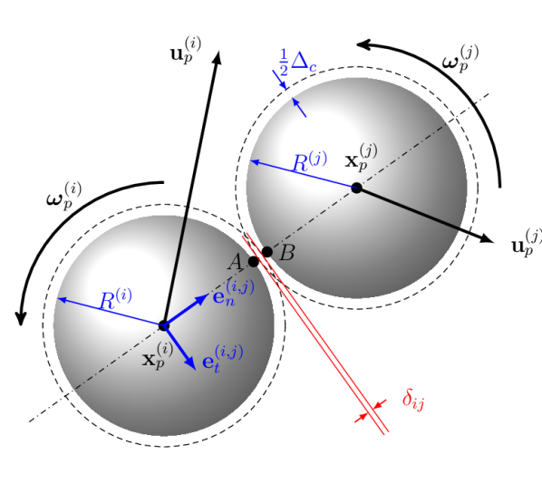
Figure 1: Schematic diagram showing two spherical particles with indices $i$ and $j$ colliding in the context of a soft-sphere collision model.

The presently employed DEM uses a standard soft-sphere approach which is based on a linear mass-spring-damper system. More specifically, let us consider a pair of particles with indices $i$ and $j$ belonging to a system with a total number of $N_{p}$ particles (for an illustration of the geometrical relations please refer to figure 1). We define an overlap length $\delta_{ij}(t)$ as follows

$$\delta_{ij}(t)=R^{(i)}+R^{(j)}+\Delta_{\rm c}-|\mathbf{x}^{(j)}_{p}(t)-\mathbf{x}^{(i)}_{p}(t)|\;,$$ (1)

where $R^{(i)}$ denotes the $i$th particle’s radius and $\mathbf{x}^{(i)}_{p}(t)$ is its center position at time $t$. The length $\Delta_{\rm c}$ in (1) is an admitted gap termed ‘force range’ by Patankar and Joseph (2001) in the context of a point-particle description coupled to a soft-sphere model. It accounts for the distance over which the actual fluid-solid interfaces are ‘smeared out’ in the discrete formulation of the fluid flow problem. Therefore, $\Delta_{c}$ is related to the support of the regularized delta function used in the context of the present immersed boundary method (Uhlmann, 2005a); its magnitude is of the order of the mesh width $\Delta x$ (precise values will be stated for each flow case below).

We can now determine whether a given particle pair with indices $i$, $j$ ($i\neq j$) is in contact at time $t$ by introducing the following function $I_{c}^{(i,j)}$:

$$I_{c}^{(i,j)}(t)=\left\{\begin{array}[]{lll}1&\mbox{if}&\delta_{ij}(t)\geq 0\;,\\ 0&\mbox{else}\;.&\end{array}\right.$$ (2)

The force $\mathbf{f}_{c}^{(i)}(t)$ acting on particle $i$ as a result of its contact with neighboring particles is then defined as

$$\mathbf{f}_{c}^{(i)}(t)=\sum_{\begin{subarray}{c}j=1\\ j\neq i\end{subarray}}^{N_{p}}\Big{(}\mathbf{f}_{el}^{(i,j)}(t)+\mathbf{f}_{d}^{(i,j)}(t)+\mathbf{f}_{t}^{(i,j)}(t)\Big{)}I_{c}^{(i,j)}(t)\;.$$ (3)

The three individual force contributions entering the contact force in (3) are modeled as follows. The elastic part $\mathbf{f}_{el}^{(i,j)}(t)$ of the normal force component is a linear function of the overlap between each particle pair. Its value (acting on the $i$th particle) is given by:

$$\mathbf{f}_{el}^{(i,j)}(t)=-k_{n}\,\delta_{ij}(t)\,\mathbf{e}_{n}^{(i,j)}(t)\;,$$ (4)

where $k_{n}$ is a constant stiffness coefficient, and $\mathbf{e}_{n}^{(i,j)}$ is the unit normal vector along the line connecting the two particle centers pointing from $\mathbf{x}^{(i)}_{p}$ to $\mathbf{x}^{(j)}_{p}$:

$$\mathbf{e}_{n}^{(i,j)}(t)=\frac{\mathbf{x}^{(j)}_{p}(t)-\mathbf{x}^{(i)}_{p}(t)}{|\mathbf{x}^{(j)}_{p}(t)-\mathbf{x}^{(i)}_{p}(t)|}\;.$$ (5)

The dissipative part $\mathbf{f}_{d}^{(i,j)}(t)$ of the normal force acting on the $i$th particle is defined as:

$$\mathbf{f}_{d}^{(i,j)}(t)=-c_{dn}\,\mathbf{u}_{r,n}^{(i,j)}(t)\;,$$ (6)

where $c_{dn}$ is a constant damping coefficient, and $\mathbf{u}_{r,n}^{(i,j)}$ is the normal component of the relative velocity of particle $i$ with respect to particle $j$ at the contacting points (cf. points $A$ and $B$ in figure 1). This relative velocity is defined as follows:

$$\mathbf{u}_{r}^{(i,j)}(t) = \mathbf{u}_{p}^{(i)}(t)-\mathbf{u}_{p}^{(j)}(t)+\boldsymbol{\omega}_{p}^{(i)}(t)\times R^{(i)}\mathbf{e}_{n}^{(i,j)}(t)+\boldsymbol{\omega}_{p}^{(j)}(t)\times R^{(j)}\mathbf{e}_{n}^{(i,j)}(t)\;,$$ (7)

$$\mathbf{u}_{r,n}^{(i,j)}(t) = \Big{(}\mathbf{e}_{n}^{(i,j)}(t)\cdot\mathbf{u}_{r}^{(i,j)}(t)\Big{)}\mathbf{e}_{n}^{(i,j)}(t).$$ (8)

The force acting tangentially (on the $i$th particle) applied at the contact points between particles $i$ and $j$ is computed according to the following expression:

$$\mathbf{f}_{t}^{(i,j)}(t)=\left\{\begin{array}[]{lll}-\Big{[}\min\big{\{}\mu_{\rm c}\big{|}\mathbf{f}_{el}^{(i,j)}(t)+\mathbf{f}_{d}^{(i,j)}(t)\big{|}\,,\,c_{dt}\big{|}\mathbf{u}_{r,t}^{(i,j)}(t)\big{|}\big{\}}\Big{]}\mathbf{e}_{t}^{(i,j)}(t)&\mbox{if}&|\mathbf{u}_{r,t}^{(i,j)}(t)|\neq 0\;,\\[20.0pt] 0&\mbox{else}\;.&\end{array}\right.$$ (9)

Relation (9) expresses the fact that the tangential frictional force with damping coefficient $c_{dt}$ is proportional to the tangential component of the relative velocity at the contact point (cf. below); it is, however, limited by the Coulomb friction, which is in turn proportional to the normal force acting at the same contact point, multiplied by a friction coefficient $\mu_{c}$. The tangential component of the relative velocity $\mathbf{u}_{r,t}^{(i,j)}(t)$ is given by the following relation:

$$\mathbf{u}_{r,t}^{(i,j)}(t)=\mathbf{u}_{r}^{(i,j)}(t)-\mathbf{u}_{r,n}^{(i,j)}(t)\;,$$ (10)

while the tangential unit vector $\mathbf{e}_{t}^{(i,j)}$ is defined as:

$$\mathbf{e}_{t}^{(i,j)}(t)=\frac{\mathbf{u}_{r,t}^{(i,j)}(t)}{|\mathbf{u}_{r,t}^{(i,j)}(t)|},\quad\forall\quad|\mathbf{u}_{r,t}^{(i,j)}(t)|\neq 0\;.$$ (11)

It is important to note that the tangential component of the collision force generates a torque. The net torque $\mathbf{t}_{c}^{(i)}$ acting on particle $i$ due to all binary collisions at time $t$ is given by:

$$\mathbf{t}_{c}^{(i)}(t)=R^{(i)}\mathbf{e}_{n}^{i,j}\times\sum_{j=1}^{N_{\rm p}}\mathbf{f}_{c}^{(i,j)}(t)I_{c}^{(i,j)}(t)\;.$$ (12)

The model described in (3-12) introduces four parameters affecting the collision process namely: $k_{n}$, $c_{dn}$, $c_{dt}$, $\mu_{c}$ as well as the above-mentioned force range $\Delta_{c}$. From an analytical solution of the linear mass-spring-damper system in an idealized configuration (considering a binary normal collision in vacuum and in the absence of external forces), a relation between the normal stiffness coefficient $k_{n}$ and the normal damping coefficient $c_{dn}$ can be found. For this purpose one can define a dry restitution coefficient $\varepsilon_{d}$ as the ratio of the post-collision to pre-collision normal relative velocities in vacuum as

$$\varepsilon_{d}=-\frac{|\mathbf{u}_{r,n}^{(i,j)}|_{post}}{|\mathbf{u}_{r,n}^{(i,j)}|_{pre}}\;.$$ (13)

With this definition, it can be shown that the following relation holds between the normal damping coefficient and the stiffness coefficient (Crowe et al., 1998):

$$c_{dn}=-2\sqrt{M_{ij}k_{n}}\frac{\ln{\varepsilon_{d}}}{\sqrt{\pi^{2}+\ln^{2}\varepsilon_{d}}}\;,$$ (14)

where $M^{(l)}$ is the mass of the $l$th particle and

$$M_{ij}=M^{(i)}M^{(j)}/(M^{(i)}+M^{(j)})$$ (15)

is the reduced mass of the particle pair $i,j$. A crucial parameter of the collision model described above is the duration of a generic collision event, since it determines the time step required to numerically integrate the Newton equations of solid body motion. It can again be shown that the duration of a collision for the ideal configuration mentioned above is given by the following formula (Crowe et al., 1998):

$$T_{c}=\frac{2\pi M_{ij}}{\sqrt{4M_{ij}k_{n}-c_{dn}^{2}}},$$ (16)

which provides a useful reference value.

The collision between a particle with index $i$ and a plane wall is treated in a similar way as the inter-particle collisions. However, in the former case we set $\mathbf{x}^{(j)}_{p}(t)$ equal to the position of the wall-contact point, set the overlap length to $\delta_{ij}(t)=R^{(i)}+\Delta_{\rm c}-|\mathbf{x}^{(j)}_{p}(t)-\mathbf{x}^{(i)}_{p}(t)|$ instead of (1), use $M_{ij}=M^{(i)}$ instead of (15), and replace the $j$th particle’s velocity by the wall velocity in (7).

Similar to Wachs (2009) we have kept the solid-solid contact model as simple as possible. For this purpose, we do not include any additional force into the formulation, such as a lubrication correction (e.g. Nguyen and Ladd, 2002).

2.3 Time discretization of the equations of particle motion

Due to the comparatively large stiffness of typical solid materials, the collision time scale $T_{c}$ is often much smaller than the typical time step of the fluid solver $\Delta t$. It is straightforward to show for the configurations considered in the present work that these two scales are typically separated by at least one order of magnitude. Taking into account the fact that ${\cal O}(10)$ time steps are typically required to accurately describe a generic collision event (Cleary and Prakash, 2004), it turns out that the ratio between fluid and solid time steps easily reaches ${\cal O}(100)$. In order to avoid this restriction, one approach is to apply a sub-stepping strategy. In this framework the Newton equations for particle motion are solved with a smaller time step $\Delta t_{sub}$ than the one used for solving the Navier-Stokes equations $\Delta t$ (see e.g. Wachs, 2009). Recently Kempe and Fröhlich (2012) have proposed a strategy of artificial collision time stretching, matching the time scale of the collision to that of the fluid. In the present work, we have adopted the former strategy of separately resolving the two time scales. Sub-stepping amounts to keeping the hydrodynamic contribution to force and torque acting on the particles constant for the duration of a number of time steps $N_{sub}$ (where $N_{sub}=\Delta t/\Delta t_{sub}$) between two consecutive updates of the fluid phase. It should be noted that the particle-related computational load is not critically limited by the collision treatment in our computational implementation. This allows us to choose a conservatively small value for $\Delta t_{sub}$. In the cases treated in the present work, the number of sub-steps was in the range of $100$-$240$.

Case	$\rho_{p}/\rho_{f}$	$Ga$	$Re_{p}$	$St$	$k_{n}^{*}$	domain
C01	2.0	30.9	21.2	4.7	40053	D1
C02	2.5	37.8	28.4	7.9	33377	D1
C03	3.0	43.7	34.9	11.6	30039	D1
C04	3.5	48.8	40.9	15.9	28037	D1
C05	4.0	53.5	46.4	20.6	26702	D1
C06	5.0	61.8	56.6	31.4	25033	D1
C07	6.0	69.1	66.0	44.0	24032	D2
C08	7.0	75.6	74.7	58.1	23364	D2
C09	8.0	81.7	82.9	73.7	22887	D2
C10	9.0	87.3	90.6	90.6	22530	D2
C11	4.0	37.8	28.4	12.6	26702	D2
C12	5.0	43.7	34.9	19.4	25033	D2
C13	6.0	48.8	40.8	27.2	23969	D2
C14	8.0	57.8	51.6	45.9	22843	D2
C15	14.0	78.7	78.5	122.2	215427	D3
C16	16.0	84.6	86.4	153.6	213406	D3
C17	18.0	90.0	93.9	187.7	211675	D3
C18	20.0	95.2	101.0	224.5	210474	D3
C19	30.0	75.1	73.9	246.3	206629	D3
C20	40.0	87.1	90.2	400.7	204997	D3
C21	50.0	97.7	105.0	583.3	204031	D3
C22	70.0	115.9	132.0	1026.7	202939	D3
C23	90.0	131.6	157.3	1573.2	202162	D3
C24	100.0	138.8	169.1	1878.3	201970	D3
C08b	7.0	75.6	74.7	58.1	23364	D2b
C08c	7.0	75.6	75.4	58.6	23364	D2c
C08d	7.0	75.6	75.4	58.6	23364	D2d

Table 1: Physical parameters of the different simulations corresponding to the vertically-oriented normal collision of a single particle with a wall in a viscous fluid. $\rho_{p}/\rho_{f}$ is the particle-to-fluid density ratio; $Ga$ is the Galileo number; $Re_{p}$ and $St$ are the particle’s Reynolds number and the Stokes number based on the particle’s terminal velocity; the normalized stiffness constant in the normal collision force is defined as $k_{n}^{\ast}=k_{n}/((\rho_{p}/\rho_{f}-1)|\mathbf{g}|V_{p}/D)$. The computational domain size and numerical parameters corresponding to the abbreviation in column 7 are listed in table 2.

Domain	$[L_{x}\times L_{y}\times L_{z}]/D$	$N_{x}\times N_{y}\times N_{z}$	$D/\Delta x$	$\Delta_{c}/\Delta x$
D1	$6.4\times 25.6\times 6.4$	$128\times 513\times 128$	20	2
D2	$6.4\times 51.2\times 6.4$	$128\times 1025\times 128$	20	2
D2b	$6.4\times 51.2\times 6.4$	$128\times 1025\times 128$	20	1
D2c	$6.4\times 51.2\times 6.4$	$192\times 1537\times 192$	30	2
D2d	$6.4\times 51.2\times 6.4$	$192\times 1537\times 192$	30	1
D3	$6.4\times 102.4\times 6.4$	$128\times 2049\times 128$	20	2

Table 2: Numerical parameters of the particle-wall rebound simulations. $L_{i}$ and $N_{i}$ are the computational domain length and number of grid points in the $i$th coordinate direction, respectively; $\Delta x$ is the uniform grid spacing and $\Delta_{\rm c}$ is the force range.

3 Collision of a sphere with a wall in a viscous fluid

3.1 Computational setup and parameter values

For validation purposes we have simulated the case of an isolated sphere settling on a straight vertical path under the action of gravity before colliding with a plane horizontal wall. The chosen setup is similar to the experiment of Gondret et al. (2002). Our computational domain has periodic boundary conditions in the wall-parallel directions $x$ and $z$, and a no-slip condition is imposed upon the fluid at the domain boundaries in the wall-normal direction $y$. Gravity is directed in the negative $y$ direction. A spherical particle of diameter $D$ is released from a position near the upper wall located at a wall-normal distance $L_{y}$ from the bottom wall. From dimensional considerations this problem is characterized by two dimensionless numbers, e.g. the solid-to-fluid density ratio $\rho_{p}/\rho_{f}$ and the Galileo number $Ga=u_{g}D/\nu$, where $u_{g}=((\rho_{p}/\rho_{f}-1)|\mathbf{g}|D)^{1/2}$, $\mathbf{g}$ being the vector of gravitational acceleration and $\nu$ the kinematic viscosity. However, the data for the particle motion under normal collision with a wall is well described as a function of the Stokes number $St$ alone (Joseph et al., 2001; Gondret et al., 2002). The Stokes number can be defined from the terminal settling velocity $v_{pT}$ of the sphere as

$$St=\frac{\rho_{p}}{\rho_{f}}\frac{Re_{T}}{9}\,,$$ (17)

where $Re_{T}=v_{pT}D/\nu$.

In the present work we have simulated $24$ different combinations of values for the density ratio and the Galileo number. These values are given in table 2.3 along with the corresponding values of the terminal Reynolds number and of the Stokes number. The present simulations cover the range of $St=4.7-1880$. The size of the computational domain as well as the grid resolution (expressed as the ratio between the particle diameter and the mesh width, $D/\Delta x$) are given in table 2. It should be pointed out that, although the flow remains axisymmetric at all times, the simulations were done with a full three-dimensional Cartesian grid with uniform mesh size. Three additional simulations (termed C08^b, C08^c, C08^d) with the same physical parameter values as in case C08 have been run in order to check the sensitivity of the results with respect to the spatial resolution and the choice of the value for the force range $\Delta_{c}$ (cf. table 2).

Concerning the parameters for the solid-solid contact model, the following values were chosen. The stiffness parameter $k_{n}$, normalized by the submerged weight of the particle divided by its diameter, varies in the range of $2\cdot 10^{4}-2\cdot 10^{5}$, cf. table 2.3. With this choice the maximum penetration distance recorded in the different simulations measures only a few percent of the force range $\Delta_{c}$ (i.e. $\max(\delta_{ij}(t))\leq 0.05\Delta_{c}$). In two of the cases (C08^b and C08^d the maximum penetration reaches a value of approximately $0.2\Delta_{c}$, which still only corresponds to one percent of the respective particle diameter. The dry coefficient of restitution was set to a value $\varepsilon_{d}=0.97$ corresponding e.g. to dry collisions of steel or glass spheres on a glass wall (Gondret et al., 2002). The normal damping coefficient $c_{n}$ was determined according to relation (14).

3.2 Results

Figure 2a shows the wall-normal particle position (scaled with the particle diameter) as a function of time (normalized with the reference time $D/v_{pT}$). It is seen that in all simulated cases the particle has attained its terminal velocity before feeling the hydrodynamic influence of the solid wall. After rebound the maximum distance between the wall and the closest point on the particle surface varies from a negligibly small value ($0.004D$) for case C01 up to approximately $40D$ for case C24. In three cases (C01, C02, C03) the maximum rebound height was below $0.04$ times the particle diameter such that the results can be qualified as ‘no rebound’; the corresponding Stokes numbers are $St=4.7$, $7.9$, $11.6$, respectively, which is in agreement with the general observation that the bouncing transition occurs at $St_{c}\approx 10$ (Gondret et al., 2002).

A typical time evolution of the wall-normal particle velocity is shown in figure 2b. The figure shows the steady settling regime before impact and the subsequent rapid deceleration phase which is followed by an acceleration phase as a result of the action of the contact force. In figure 2b one can also observe the effect of the hydrodynamic forces the particle experiences just before and after the collision event.

(a)

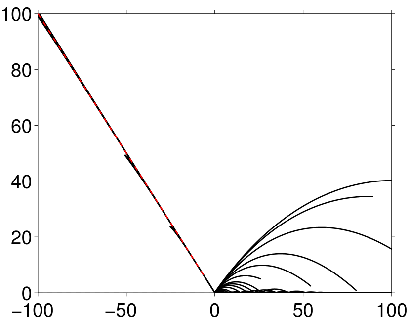
$(t-t_{1})v_{pT}/D$

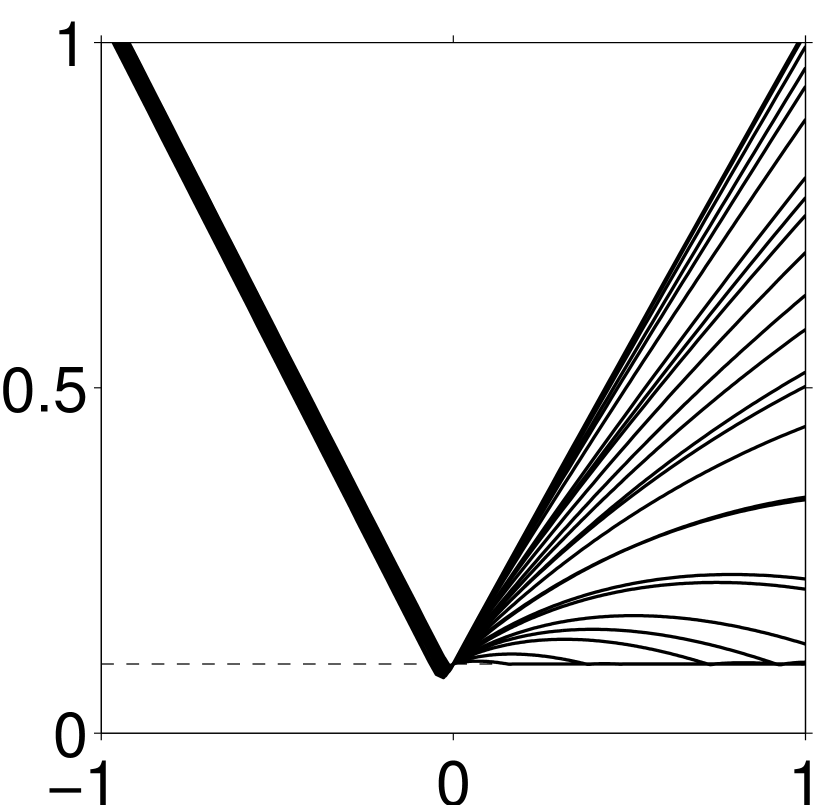
$(y_{p}-D/2)/D$

$v_{p}/v_{pT}$

(b)

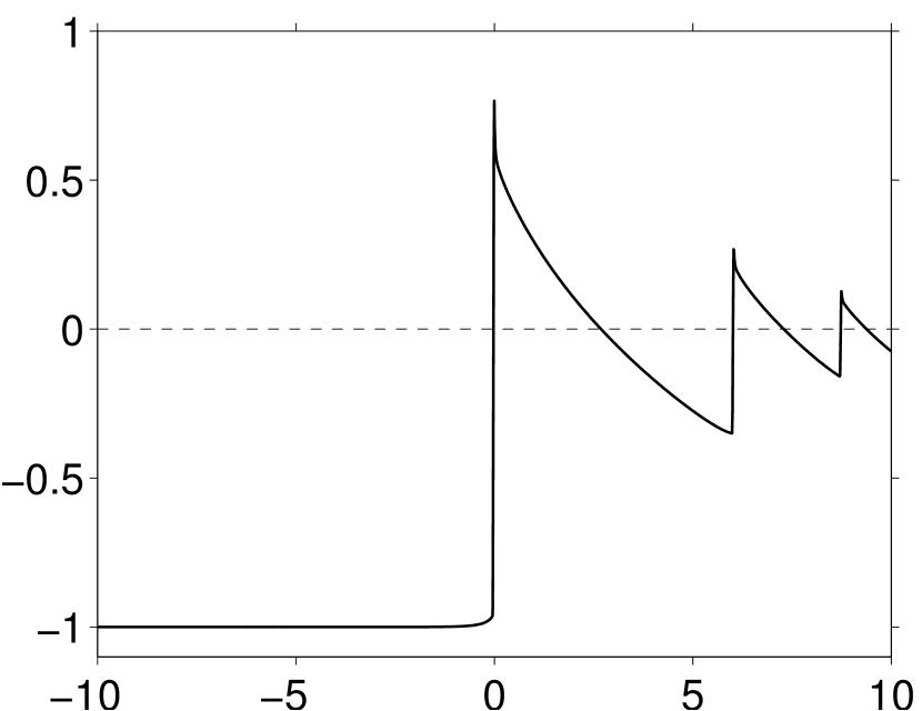
$(t-t_{1})v_{pT}/D$

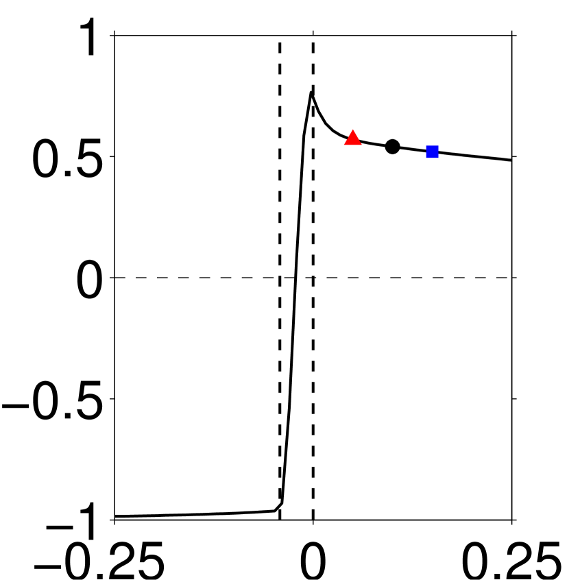
Figure 2: (a) Wall-normal position of the lowest point of the sphere $y_{p}-D/2$ as a function of time. In each case the time coordinate is shifted such that all particle impacts coincide with the origin of the graph. The red dotted line has a slope of $-1$, corresponding to motion at the terminal velocity. The horizontal dashed line in the inset indicates the $\Delta_{c}$ offset which is the extent of the collision force. (b) Wall-normal velocity of the particle in case C08 as a function of time. The symbols mark the particle rebound velocity for different values of the time delay: ($\blacktriangle$) $t_{R}=0.05D/v_{pT}$; (${{{\bullet}}}$) $t_{R}=0.1D/v_{pT}$; ($\blacksquare$) $t_{R}=0.15D/v_{pT}$. The vertical dashed lines mark the interval during which the collision force is non-zero.

One of the principal quantities of interest in this case is the effective coefficient of restitution $\varepsilon$, defined as the ratio of the particle velocity values before and after the collision, viz:

$$\varepsilon=-\frac{v_{pR}}{v_{pT}}\,.$$ (18)

In collision experiments in a viscous fluid the determination of the rebound velocity $v_{pR}$ is a somewhat delicate issue, and no unique definition seems to exist in the literature. In laboratory experiments this quantity is typically computed from measured particle position data, involving some kind of gradient computation based on the records in the direct vicinity of the wall. Therefore, the result may be sensitive to the temporal resolution of the measuring device. In the experiment of Gondret et al. (2002) the time interval between successive images was $2\,ms$ which means the first data point after impact was recorded approximately at a time of $0.3D/v_{pT}$ after the particle loses contact with the wall (under typical conditions of their experiment). In the experiment of Joseph et al. (2001), which featured a pendulum set-up with a horizontal impact on a vertical wall, the temporal resolution was comparably higher, corresponding to approximately $0.03D/v_{pT}$. In both cases the temporal resolution is significantly larger than the duration of the actual collision. As a consequence, the measured rebound velocity $v_{pR}$ (and therefore the effective coefficient of restitution $\varepsilon$) takes into account to some extent the fluid-induced damping after the particle-wall contact.

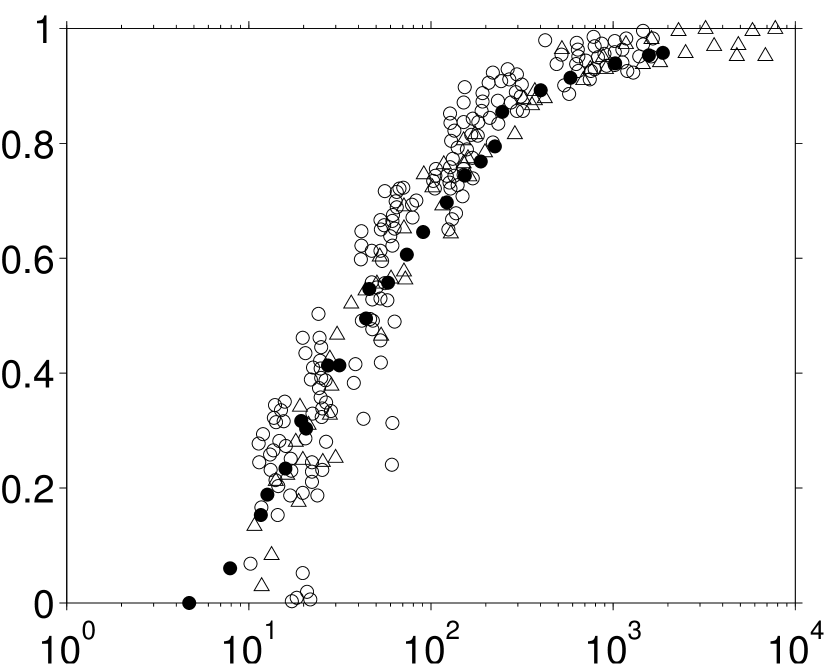
$St$

$\varepsilon/\varepsilon_{d}$

Figure 3: Ratio between the effective coefficient of restitution $\varepsilon$ and the dry value $\varepsilon_{d}$ as a function of the Stokes number. The present results are indicated by the symbols (${{{\bullet}}}$), and the rebound velocity has been computed from (19) with $t_{R}=0.1D/v_{pT}$. Experimental data of Joseph et al. (2001) and Gondret et al. (2002) are marked by the symbols (${{{\circ}}}$) and ($\vartriangle$) respectively.

(a)

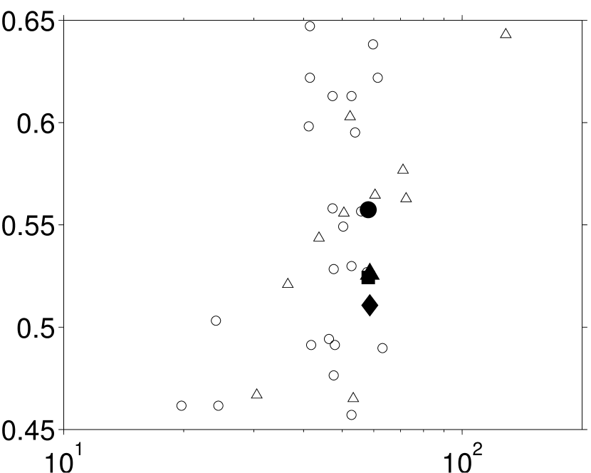
$St$

$\varepsilon/\varepsilon_{d}$

$\varepsilon/\varepsilon_{d}$

(b)

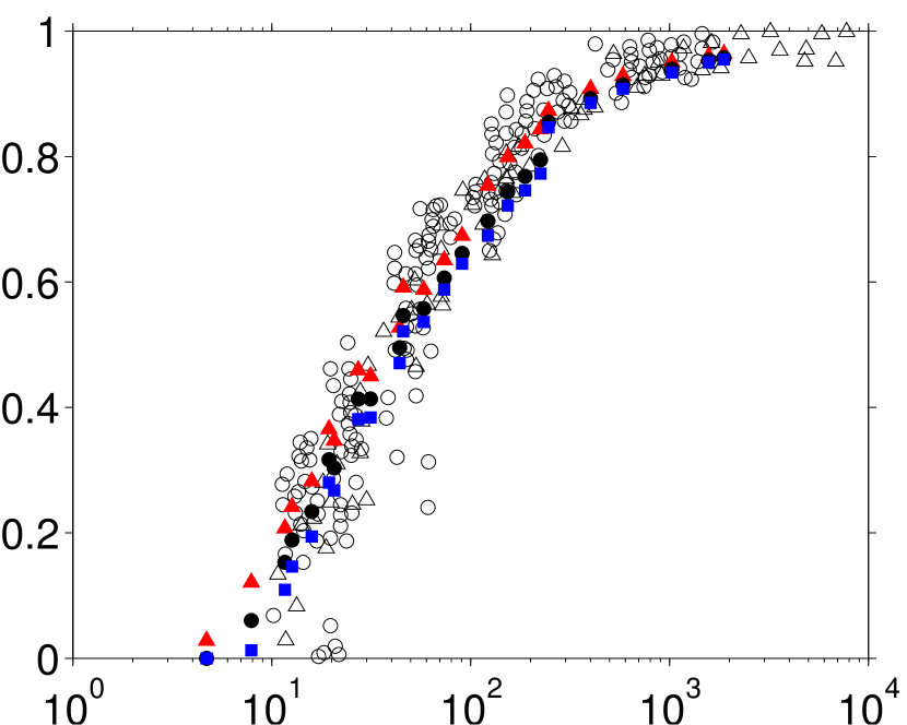
$St$

Figure 4: (a) Sensitivity of the computed effective coefficient of restitution with respect to the numerical parameters for $\rho_{p}/\rho_{f}=7$ and $Ga=75.6$: (${{{\bullet}}}$) case C08 ($D/\Delta x=20$, $\Delta_{c}/\Delta x=2$); (${\blacksquare}$) case C08^b ($D/\Delta x=20$, $\Delta_{c}/\Delta x=1$); ($\blacktriangle$) case C08^c ($D/\Delta x=30$, $\Delta_{c}/\Delta x=2$); ($\blacklozenge$) case C08^d ($D/\Delta x=30$, $\Delta_{c}/\Delta x=1$). (b) Sensitivity of $\varepsilon$ with respect of the chosen value for the delay time $t_{R}$ for all simulations: ($\blacktriangle$) $t_{R}=0.05D/v_{pT}$; (${{{\bullet}}}$) $t_{R}=0.1D/v_{pT}$; (${\blacksquare}$) $t_{R}=0.15D/v_{pT}$. In both graphs the symbols (${{{\circ}}}$) and ($\vartriangle$) correspond to the experimental data of Joseph et al. (2001) and Gondret et al. (2002), respectively.

In the present work we measure the rebound velocity at a predefined time after the particle loses contact with the wall. More precisely, we define

$$v_{pR}=v_{p}(t_{1}+t_{R})\,,$$ (19)

where $t_{1}$ is the instant in time when the contact force first becomes zero after the particle-wall collision, and $t_{R}$ is a prescribed delay which was set to the value of $t_{R}=0.1D/v_{pT}$. Note that the chosen value for the delay is comparable to the one used in the work of Gondret et al. (2002). The insert in figure 2b shows the time evolution of the particle velocity around the collision interval in the present case C08, where the rebound velocity obtained from the definition in (19) is marked by a symbol. Also shown in that figure are two alternative choices of delay times ($t_{R}\,v_{pT}/D=0.05$ and $0.15$) which will be further discussed below.

The effective coefficient of restitution computed according to (18) is shown as a function of the Stokes number in figure 3. A very good match with the data points provided by the experimental measurements of Gondret et al. (2002) and those of Joseph et al. (2001) can be observed over the whole parameter range, with an exponential increase in $\varepsilon$ beyond $St_{c}\approx 10$. This result demonstrates that the comparatively simple collision model employed in the present work is capable of accurately reproducing the fluid-mediated impact of a spherical particle on a solid wall in the framework of an immersed boundary technique.

The results obtained in the additional simulations C08^b, C08^c, C08^d are shown in figure 4$(a)$ in comparison to the original case C08 (all four simulations are for $\rho_{p}/\rho_{f}=7$ and $Ga=75.6$). In simulation C08^b the grid resolution is kept the same as in case C08 ($D/\Delta x=20$), but the force range $\Delta_{c}$ is divided by two. The result is a reduction of the effective coefficient of restitution by approximately 6%. Nearly the same effect is obtained in case C08^c where the force range is maintained constant (in multiples of the mesh width), but the spatial resolution is increased to $D/\Delta x=30$. When setting the smaller value for the force range ($\Delta_{c}/\Delta x=1$) and simultaneously choosing the decreased mesh width ($D/\Delta x=30$) as in case C08^d, a reduction of the value of $\varepsilon$ by approximately 9% is obtained. In comparison to the available experimental data, this sensitivity analysis shows that the value of the force range is not a crucial quantity. It also demonstrates that a mesh width of $D/\Delta x=20$ is adequate at the present parameter point.

Finally, let us consider the sensitivity of our results with respect to the choice of the delay time $t_{R}$. For all present simulations figure 4$(b)$ shows the results for the effective coefficient of restitution computed with three different values of the delay time as indicated in figure 2$(b)$: $t_{R}\,v_{pT}/D=0.05$, $0.1$ and $0.15$. Choosing a smaller delay time has the effect of systematically increasing the coefficient of restitution, since the fluid-mediated damping after the particle-wall contact has less time to act. However, it can be observed that over the whole range of values the simulation results match the experimental data very well.

4 Erosion of granular bed sheared by laminar flow

4.1 Computational setup

4.1.1 Flow configuration and parameter values

$(a)$                                       $(b)$

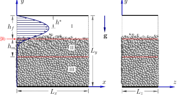
Figure 5: Schematic diagram showing the configuration of the bedload transport simulations in § 4. Periodicity in the $x$- and $z$-directions is assumed. $(a)$ shows the streamwise/wall-normal plane; in $(b)$ the view is into the streamwise direction.

In the present section we are considering the motion of spherical particles induced by laminar flow in a horizontal plane channel, as sketched in figure 5. The computational set-up features a number of particles ($N_{p}$) forming a sediment bed which takes up a large fraction of the channel height. As figure 5 shows, the Cartesian coordinates $x$, $y$, and $z$ correspond to the streamwise, wall-normal and spanwise directions, respectively. The cuboidal computational domain is of size $L_{x}$, $L_{y}$, $L_{z}$ in the respective coordinate directions; periodicity is imposed in $x$ and $z$, while a no-slip condition is applied at the two wall planes. The flow is driven by a streamwise pressure gradient adjusted at each time step such as to maintain a constant flow rate $q_{f}$ (note that the actual volumetric flow rate is divided by the spanwise domain size, i.e. $q_{f}$ corresponds to a flow rate per unit span with units of velocity times length). The particulate flow problem features 10 relevant quantities ($\rho_{p}$, $\rho_{f}$, $q_{f}$, $|\mathbf{g}|$, $D$, $\nu$, $L_{x}$, $L_{y}$, $L_{z}$, $N_{p}$) which means that it is fully described by 7 non-dimensional parameters. These can be chosen as follows: the particle-to-fluid density ratio $\rho_{p}/\rho_{f}$; the Galileo number $Ga$ (defined in § 3.1); the bulk Reynolds number given by

$$Re=\frac{q_{f}}{\nu}\,;$$ (20)

the global solid volume fraction defined as

$$\Phi_{s}=\frac{N_{p}V_{p}}{L_{x}L_{y}L_{z}}\,,$$ (21)

where $V_{p}=(\pi/6)D^{3}$ is the particle volume; the three relative length scales $L_{x}/D$, $L_{y}/D$, $L_{z}/D$. As an alternative to one of the latter length scale ratios one can e.g. choose an imposed pile height parameter given by (Silbert et al., 2001)

$$H_{b}=N_{p}D^{2}/(L_{x}\,L_{z})\,.$$ (22)

Table 3: Physical parameters of the bedload transport simulations in § 4: bulk Reynolds number $Re$, Galileo number $Ga$, normalized solid stiffness coefficient $k_{n}^{\ast}=k_{n}D/((\rho_{p}/\rho_{f}-1)V_{p}|\mathbf{g}|)$, pile height parameter $H_{b}$ (given in 22), global solid volume fraction $\Phi_{s}$ (defined in 21), number of particles $N_{p}$, fluid height $h_{f}$ (as defined in § 4.1.4), Shields number $\Theta_{Pois}$ (defined in 24) and solid volume fraction inside the bulk of the bed $\Phi_{bed}$ (as defined in 27). The particle-to-fluid density ratio was kept at $\rho_{p}/\rho_{f}=2.5$ in all cases. The computational domain size and numerical parameters corresponding to the abbreviation in column 11 are listed in table 4.

Domain	$[L_{x}\times L_{y}\times L_{z}]/D$	$N_{x}\times N_{y}\times N_{z}$	$D/\Delta x$	$\Delta_{c}/\Delta x$	symbol
D4	$32\times 32\times 16$	$512\times 513\times 256$	16	2	,${{{\bullet}}}$
D5	$32\times 36\times 16$	$512\times 577\times 256$	16	2	,${{{\bullet}}}$
D6	$32\times 16\times 16$	$512\times 257\times 256$	16	2	,${{{\bullet}}}$
D7	$38.4\times 25.6\times 12.8$	$384\times 257\times 128$	10	1	,${\blacksquare}$
D8	$38.4\times 51.2\times 12.8$	$384\times 513\times 128$	10	1	,${\blacksquare}$
D8b	$38.4\times 51.2\times 12.8$	$768\times 1025\times 256$	20	2	,$\blacktriangle$
D9	$32\times 36\times 16$	$512\times 577\times 256$	16	1	,$\blacklozenge$
D10	$32\times 32\times 16$	$512\times 513\times 256$	16	1	,$\blacklozenge$

Table 4: Numerical parameters used in the simulations of bedload transport (for the notation cf. table 2). The color and symbol coding given in the last column correspond to a chosen pair of numerical parameter values ($D/\Delta x$,$\Delta_{c}/\Delta x$) and will be used in subsequent plots.

Further global parameters of interest are computed a posteriori from the observed height $h_{f}$ of the fluid-bed interface (defined in § 4.1.4) as well as from the characteristic shear stress. The Shields number is defined as

$$\Theta=\frac{u_{\tau}^{2}}{\left(\rho_{p}/\rho_{f}-1\right)|\mathbf{g}|D}\,,$$ (23)

where $u_{\tau}=(\tau_{w}/\rho_{f})^{1/2}$ is the friction velocity (with $\tau_{w}$ denoting the wall shear stress). In laminar plane Poiseuille flow with smooth walls, the Shields number can be written as (using the present notation):

$$\Theta_{Pois}=\frac{6\,Re}{Ga^{2}}\,\left(\frac{D}{h_{f}}\right)^{2}\,.$$ (24)

Although in a region near the rough fluid-bed surface the mean velocity profile is not identical to a parabolic Poiseuille profile (cf. discussion in § 4.2.4), the Shields number based upon the definition (24) is often used as a parameter in experimental studies. Therefore, its value is included in table 2.3 for each simulated case.

Out of the total number of $N_{p}$ particles, one layer adjacent to the wall (in dense hexagonal arrangement and with a vertical displacement by one particle radius applied to every second particle in that layer) is kept fixed during the entire simulation in order to form a rough bottom wall surface. The chosen parameter values in the 26 independent simulations which we have performed are listed in table 2.3. Note that 24 different physical parameter combinations have been chosen. The remaining two simulations (B20^b and B21^b) were conducted at one half the mesh width in order to verify the adequacy of the spatial resolution.

Let us now turn to the parameter values of the solid contact model. Analogous to the strategy employed in § 3.1 we have set the stiffness parameter $k_{n}$ of the elastic normal force component such that the maximum penetration length is kept below a few percent of the force range (i.e. $\max(\delta_{ij}(t))\leq 0.05\Delta_{c}$). This criterion is fulfilled for values of $k_{n}^{\ast}=k_{n}D/((\rho_{p}/\rho_{f}-1)V_{p}|\mathbf{g}|)$ in the interval of $5400-17000$ (for the precise choice per flow case cf. table 2.3). The dry restitution coefficient was set to a value of $\varepsilon_{d}=0.3$, which is smaller than the material property commonly reported for glass ($\varepsilon_{d}=0.97$, cf. § 3.1) or plexiglass (PMMA, $\varepsilon_{d}=0.8$, cf.  Constantinides et al., 2008). With this choice the normal damping coefficient $c_{dn}$ can be computed from relation (14). The tangential damping coefficient was set to the same value, i.e. $c_{dt}=c_{dn}$ (Tsuji et al., 1993). The value for the Coulomb friction coefficient was fixed at $\mu_{c}=0.4$ which is similar to but somewhat larger than values reported for wet contact between glass-like materials (Foerster et al., 1994; Joseph and Hunt, 2004).

$(a)$

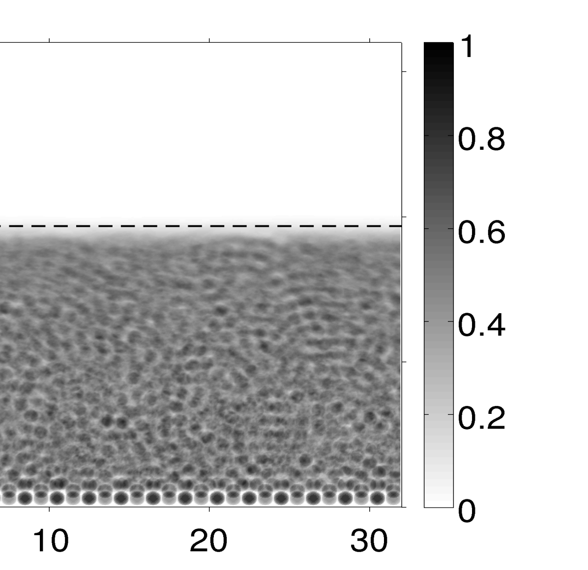
$x/D$

$y/D$

$(y-y_{0})/h_{f}$

$(b)$

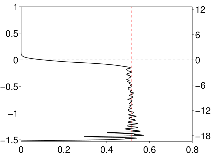
$\langle\phi_{p}\rangle$

$(y-y_{0})/D$

Figure 6: (a) Solid volume fraction averaged in time and over the spanwise direction, $\langle\phi_{p}\rangle_{zt}(x,y)$, in case BL24. The horizontal dashed line represents the mean fluid-bed interface location $y_{0}$ defined in (25). (b) The corresponding profile of the mean solid volume fraction $\langle\phi_{p}\rangle(y)$. The mean value in the bulk of the bed, $\Phi_{bed}$, is indicated by a vertical dashed line (in red color).

4.1.2 Simulation start-up and initial transient

As an initial condition for each fluid-solid simulation a sediment bed composed of quasi-randomly packed particles is generated. For this purpose, a DEM simulation was performed under the conditions of each simulation (i.e. regarding domain size, number of particles, particle diameter, particle density, value of gravitational acceleration and contact model parameters) but ignoring hydrodynamic forces, i.e. considering dry granular flow with gravity. Each DNS-DEM simulation is then started by ramping up the flow rate from zero to its prescribed value over a short time interval of the order of $10^{-2}$ bulk time units $T_{b}=h_{f}^{2}/q_{f}$ (where $h_{f}$ is the fluid height defined in § 4.1.4). After an initial transient, a statistically stationary state of the particle-fluid system is reached with – upon average – constant bed height and constant mean particle flux. The time evolution of the instantaneous particle flux $q_{p}$ (cf. equation (28) and figure 7, discussed below) is used to determine the statistically stationary state interval which is used to compute statistics.

4.1.3 Reference experimental data

A detailed set of experimental data in a similar configuration studied by Aussillous et al. (2013) is available for validation purposes. In the experiment the transport of spherical particles in a rectangular channel in the laminar regime is considered. Two combinations of fluid and particle properties were investigated by the authors with particle-to-fluid density ratios $\rho_{p}/\rho_{f}=1.11$ and $2.10$ as well as Galileo number values $Ga=0.36$ and $0.38$. A pump is used to impose a constant flow rate, which is varied such that the bulk Reynolds number ranges from $Re=0.27$ up to $1.12$. Note that these values are two orders of magnitude smaller than the Reynolds number values in the present simulations. However, the main control parameter of the problem (the Shields number) covers a similar range ($\Theta_{Pois}\approx 0.2-1$) as the present simulations. Contrary to our simulation setup, the sediment bed thickness is not kept constant in the experiment. First, a given amount of sediment is filled into the channel yielding the initial sediment bed height. After start-up of the flow, particles are eroded and transported out of the test section, resulting in a fluid height which increases with time until it reaches its final equilibrium value. Before the cessation of particle erosion is reached, statistics are accumulated at intervals of $5\,s$ (averaged over a small time window of $0.5\,s$) in which the flow is assumed to be steady. An index matching technique is utilized in order to perform optical measurements of both the velocity of the fluid phase and that of the particle phase, including locations deep inside the sediment bed.

4.1.4 Determination of the fluid height

$(a)$

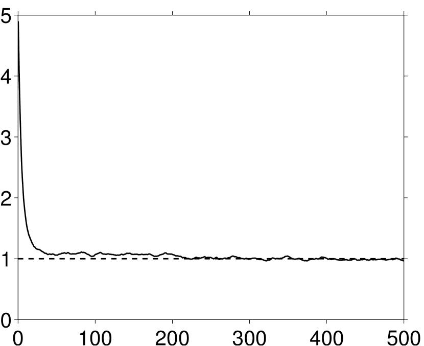
$t\,q_{\rm f}/h_{\rm f}^{2}$

$q_{p}/\langle q_{p}\rangle$

$q_{p}/\langle q_{p}\rangle$

$(b)$

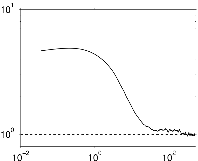
$t\,q_{\rm f}/h_{\rm f}^{2}$

Figure 7: $(a)$ Time evolution of the particle flow rate $q_{p}$ defined in (28) for case BL08, normalized by the mean value in the statistically stationary regime. $(b)$ shows the same data in logarithmic scale.

In the reference experiments, a flourescent dye is mixed into the fluid which upon illumination by a laser sheet emits light detectable by a camera. In the recorded images the particle positions show up as low intensity (i.e. dark) regions. Such an intensity map can then be averaged over a number of frames and converted into a vertical profile of the solid volume fraction; by means of thresholding the fluid-bed interface location can be determined (Lobkovsky et al., 2008; Aussillous et al., 2013). Here we have adopted the same approach to determine the location of the interface based upon our DNS-DEM simulation data. In this manner we can directly compare our results with the experimental counterpart.

In this spirit we first define a solid phase indicator function $\phi_{p}(\mathbf{x},t)$ which equals unity for a point $\mathbf{x}$ that is located inside any particle at time $t$ and zero otherwise (cf. appendix B). Next we compute the average of $\phi_{p}(\mathbf{x},t)$ over time (in the statistically stationary interval) and over the spanwise direction, yielding $\langle\phi_{p}\rangle_{zt}(x,y)$. An example of this two-dimensional map for case BL24 is shown in figure 6$(a)$. Further averaging of $\langle\phi_{p}\rangle_{zt}(x,y)$ over the streamwise direction yields the wall-normal profile of the mean solid volume fraction $\langle\phi_{p}\rangle(y)$, an example of which is given in figure 6$(b)$. Note that the angular brackets without subscripts $\langle\,\rangle$ denote an average over the two homogeneous space directions $x$, $z$ and over time. The mean solid volume fraction $\langle\phi_{p}\rangle(y)$ is an alternative quantity to $\langle\phi_{\rm s}\rangle(y)$ which is computed from the number density of particles in wall-normal averaging bins of finite size (cf. appendix B). The former approach gives more precise results in cases when there exists a strong gradient in the solid volume fraction profile as in figure 6; it is therefore generally preferred. The latter quantity enters the definition of the particle flux as defined in equation (28) below. Finally, the fluid-bed interface location is defined as the wall-normal coordinate $y_{0}$ where the value of the mean solid volume fraction equals a prescribed threshold value $\langle\phi_{p}\rangle^{thresh}=0.10$, viz.

$$y_{0} = y\;\;|\;\langle\phi_{p}\rangle(y)=\langle\phi_{p}\rangle^{thresh}\;.$$ (25)

Consequently, the fluid height is given by

$$h_{f}=L_{y}-y_{0}.$$ (26)

For the example of case BL24 the resulting interface location is shown in figure 6.

It can also be seen in figure 6$(b)$ that a reasonable value for the mean solid volume fraction in the bulk of the sediment bed can be defined as the following average

$$\Phi_{bed}=\frac{1}{y_{2}-y_{1}}\,\int_{y_{1}}^{y_{2}}\langle\phi_{p}\rangle\,\mbox{d}y\,,$$ (27)

where the interval is delimited by $y_{1}=3D$ and $y_{2}=6D$. The resulting values of $\Phi_{bed}$ vary between $0.43$ and $0.53$ as reported in table 2.3. Due to the combined effects of considering exactly mono-dispersed particles and using a finite force range $\Delta_{c}$ introduced into the collision model (cf. § 2.2), these values are somewhat smaller than what is found in experiments. For instance, in the study of Aussillous et al. (2013) values in the range of $\Phi_{bed}=0.55-0.62$ are measured while Lobkovsky et al. (2008) report $\Phi_{bed}=0.5-0.6$. Note that the maximum packing fraction of a homogeneously sheared assembly of frictional spheres measures $0.585$ (Boyer et al., 2011).

4.2 Results

4.2.1 Particle flux

           $(a)$

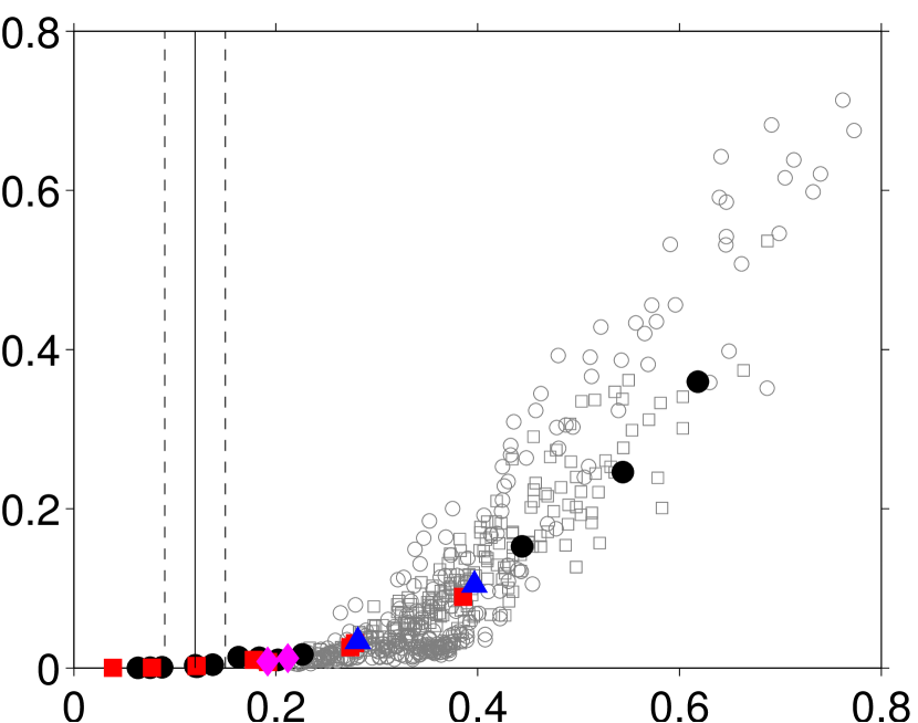
$\Theta_{Pois}$

$\langle q_{p}\rangle/q_{visc,D}$

$\langle q_{p}\rangle/q_{visc,h}$

           $(b)$

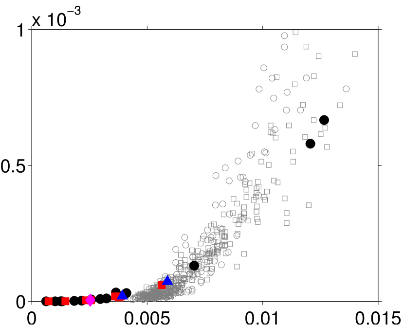
$q_{f}/q_{visc,h}$

Figure 8: ($a$) Mean particle flow rate $\langle q_{p}\rangle$ non-dimensionalized by the viscous scaling $q_{visc,D}$ plotted as a function of the Shields number $\Theta_{Pois}$. The vertical solid line corresponds to the critical Shields number for particle erosion $\Theta_{Pois}^{c}~{}=~{}0.12~{}\pm~{}0.03$ reported by Ouriemi et al. (2007), the dashed lines indicating the tolerance range. The inset shows the same data plotted in logarithmic scale. The black chain-dotted line in the inset corresponds to a power law $\langle q_{p}\rangle/q_{visc,D}~{}=~{}1.6584\Theta_{Pois}^{3.08}$. ($b$) The same quantity $\langle q_{p}\rangle$ as in $(a)$, but normalized by $q_{visc,h}$ and plotted as a function of the non-dimensional fluid flow rate $q_{f}/q_{visc,h}$. The power law $\langle q_{p}\rangle/q_{visc,h}~{}=~{}1055.3(q_{f}/q_{visc,h})^{3.21}$ is indicated by the black chain-dotted line. In both graphs the results from the present simulations are indicated by the symbols given in table 4. Data points marked by (${{{\circ}}}$,${\square}$) correspond to the experiment of Aussillous et al. (2013) (${{{\circ}}}$, combination “A” of materials in their table 1; ${\square}$, combination “B”).

In all the simulations performed in the present work the flow remains laminar. Nevertheless, the individual particle motion is highly unsteady, exhibiting sliding, rolling, reptation, and to a lesser degree saltation, within and in the vicinity of the mobile layer of the sediment bed. It is only occasionally that particles are suspended in the flow over longer times. Therefore, transport of particles as suspended load is insignificant in the present configuration, and hereafter we will not further distinguish the particle flux due to the different modes.

The instantaneous volumetric flow rate of the particle phase (per unit span), $q_{p}(t)$, is given by the sum (over all particles) of the streamwise particle velocity times the particle volume, divided by the product of the streamwise and spanwise extent of the domain, viz.

$$q_{p}(t)\;=\;\frac{\pi D^{3}}{6L_{x}L_{z}}\sum_{l=1}^{N_{p}}u_{p}^{(l)}(t)\,.$$ (28)

In (28) $u_{p}^{(l)}(t)$ denotes the streamwise component of the velocity of the $l$th particle at time $t$. Note that the quantity $q_{p}$ is termed ‘grain flux’ by Lobkovsky et al. (2008) who define it as the wall-normal integral over the product between the streamwise particle velocity and the solid volume fraction.

The time evolution of $q_{p}$ for case BL08 is shown in figure 7. It can be seen that after initialization of the flow the particle flow rate decreases from an initially large value, tending towards a statistically stationary state with a mean value $\langle q_{p}\rangle$. The duration of the transient varies among the different simulations. Since the focus of the present work is the fully developed regime, no attempt was made to find an appropriate scaling for the transient time.

Figure 8($a$) shows the mean particle flow rate in the statistically stationary regime, $\langle q_{p}\rangle$, plotted for all cases as a function of the Shields number $\Theta_{Pois}$. The experimentally determined critical value for the Shields number in the laminar flow regime, $\Theta_{Pois}^{(c)}=0.12$, together with the confidence interval $\pm 0.03$ (Ouriemi et al., 2007) are indicated with vertical lines in figure 8($a$). One possible reference quantity for the particle flow rate is the following viscous scale as suggested by Aussillous et al. (2013),

$$q_{visc,D}=\frac{(\rho_{p}/\rho_{f}-1)gD^{3}}{\nu}=Ga^{2}\,\nu\,,$$ (29)

which is equivalent to $18U_{s}D$, where $U_{s}$ is the Stokes settling velocity of a single particle. The quantity defined in (29) is used to non-dimensionalize $\langle q_{p}\rangle$ in figure 8($a$), while an alternative normalization will be explored in figure 8($b$). It is clearly observable from figure 8($a$) that the particle flow rate obtained from the present DNS-DEM is negligibly small for values of $\Theta_{Pois}\lesssim 0.12$ in good agreement with what is reported in the literature (cf. Charru et al., 2004; Loiseleux et al., 2005; Ouriemi et al., 2009). Animations of the particle motion (as provided in the supplementary material, cf. appendix A) confirm this finding. Those supplementary movies also show the well-known intermittent erratic movement of a small number of particles for Shields number values smaller than $\Theta_{Pois}^{(c)}$, as has been observed experimentally (Charru et al., 2004). On the other hand, in those runs in which the value of the Shields number is above the critical value, the particles near the fluid-bed interface are observed to be continuously in motion. The magnitude of the saturated particle flux $\langle q_{p}\rangle$ monotonically increases with increasing value of $\Theta_{Pois}$. This trend is clearly seen in figure 8($a$). The corresponding experimental data of Aussillous et al. (2013) is also added to the figure, exhibiting a very good agreement with our present DNS-DEM results. Moreover, a fit of the simulation data in figure 8($a$) for super-critical parameter points ($\Theta_{Pois}>\Theta_{Pois}^{(c)}$) yields the following power law relation: $\langle q_{p}\rangle/q_{visc,D}\propto\Theta_{Pois}^{3.08}$. Ouriemi et al. (2009) have described the present bedload transport system by means of a two-fluid model which makes use of the Einstein effective viscosity. They have shown that above the critical value $\Theta_{Pois}^{(c)}$ the model predicts a variation of the particle flow rate with the third power of the Shields number. As can be seen from the fit in figure 8($a$), their conclusion is fully confirmed by the present data.

An alternative scaling of the particle flow rate data is to replace the particle diameter in (29) with the fluid height, viz.

$$q_{visc,h}=\frac{(\rho_{p}/\rho_{f}-1)gh_{f}^{3}}{\nu}=q_{visc,D}\,\left(\frac{h_{f}}{D}\right)^{3}\;.$$ (30)

This scaling was advocated by Aussillous et al. (2013) as more consistent with a continuum (two-fluid) approach. Figure 8$(b)$ shows that our data for the particle flow rate as a function of the fluid flow rate, both normalized with the scale defined in equation (30), again matches the experimental data of Aussillous et al. (2013) very well. We also note that the simulation data is very well represented by the power law $\langle q_{p}\rangle/q_{visc,h}~{}\propto~{}(q_{f}/q_{visc,h})^{3.21}$ which is again close to a cubic variation. In fact it can be shown that a cubic variation of $\langle q_{p}\rangle/q_{visc,h}$ with $q_{f}/q_{visc,h}$ follows directly from a cubic variation of $\langle q_{p}\rangle/q_{visc,D}$ with $\Theta_{Pois}$.

$(a)$

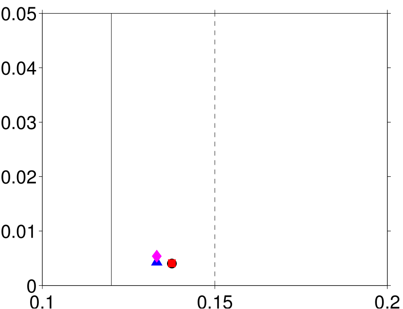
$\Theta_{Pois}$

$\langle q_{p}\rangle/q_{visc,D}$

$\langle q_{p}\rangle/q_{visc,D}$

$(a)$

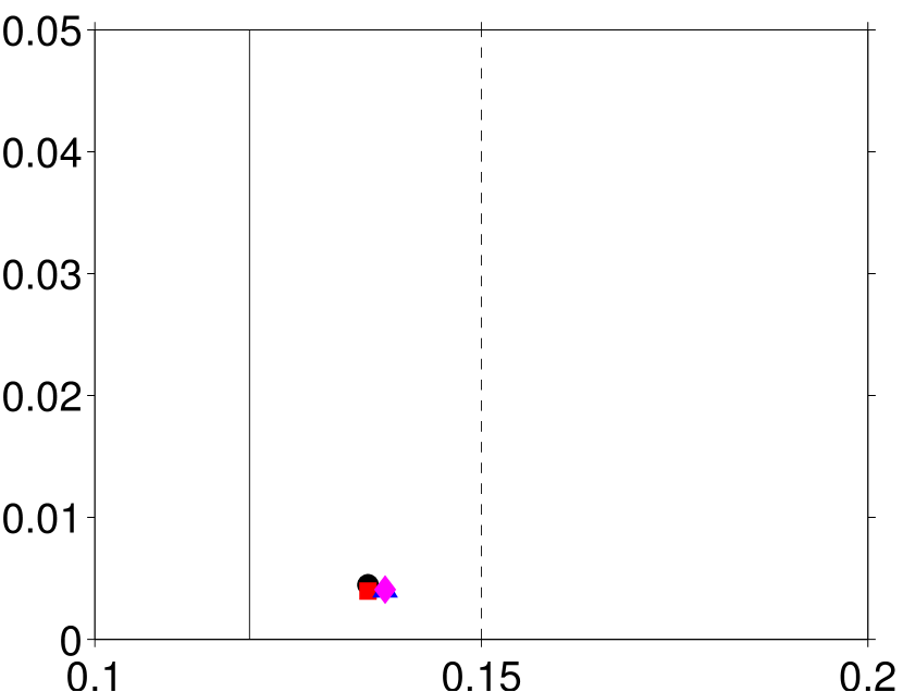
$\Theta_{Pois}$

Figure 9: As figure 8$(a)$, but showing the effect of changing the parameters of the collision model in case BL10 with $Re_{b}=266$ and $Ga=13.98$ (cf. table 2.3). In $(a)$ the dry restitution coefficient $\varepsilon_{d}$ is varied while all remaining physical and numerical parameters values are maintained: $\bullet$, $\varepsilon_{d}=0.30$; $\blacksquare$, $\varepsilon_{d}=0.60$; $\blacktriangle$, $\varepsilon_{d}=0.90$; $\blacklozenge$, $\varepsilon_{d}=0.97$. In $(b)$ only the Coulomb friction coefficient $\mu_{c}$ is varied: $\bullet$, $\mu_{c}=0.1$; $\blacksquare$, $\mu_{c}=0.25$; $\blacktriangle$, $\mu_{c}=0.4$; $\blacklozenge$, $\mu_{c}=0.55$. Note that the present axis scales are different than in figure 8$(a)$.

4.2.2 Sensitivity with respect to collision model parameters

The force range $\Delta_{c}$ has been varied by a factor of two (from $\Delta_{c}=\Delta x$ to $\Delta_{c}=2\Delta x$) in two simulation cases (BL20 and BL21, where $Re_{b}=267$ and $333$, respectively, and $Ga=6.3$ in both cases, cf. tables 2.3 and 4). It can be seen from figure 8 that the effect of modifying this parameter upon the particle flow rate is insignificant in the given range. The same conclusion holds for the quantities discussed below (§ 4.2.3-4.2.4).

We have likewise tested the influence of the choice of the value for the dry restitution coefficient $\varepsilon_{d}$ upon the results in the present configuration. For this purpose the flow case denoted BL10 in table 2.3 has been repeated three times with modified values of the dry restitution coefficient (while maintaining all remaining numerical and physical parameters at their original value). Figure 9$(a)$ shows the resulting mean particle flow rate for the set of coefficients $\varepsilon_{d}=0.3$, $0.6$, $0.9$, $0.97$. As can be observed, the impact of this parameter variation is very limited.

Finally, we have repeated the same case BL10 while independently changing the value of the Coulomb friction coefficient in the range $\mu_{c}=0.1\ldots 0.55$. The result is shown in figure 9$(b)$, where again a very small effect upon the mean particle flow rate is obtained.

           $(a)$

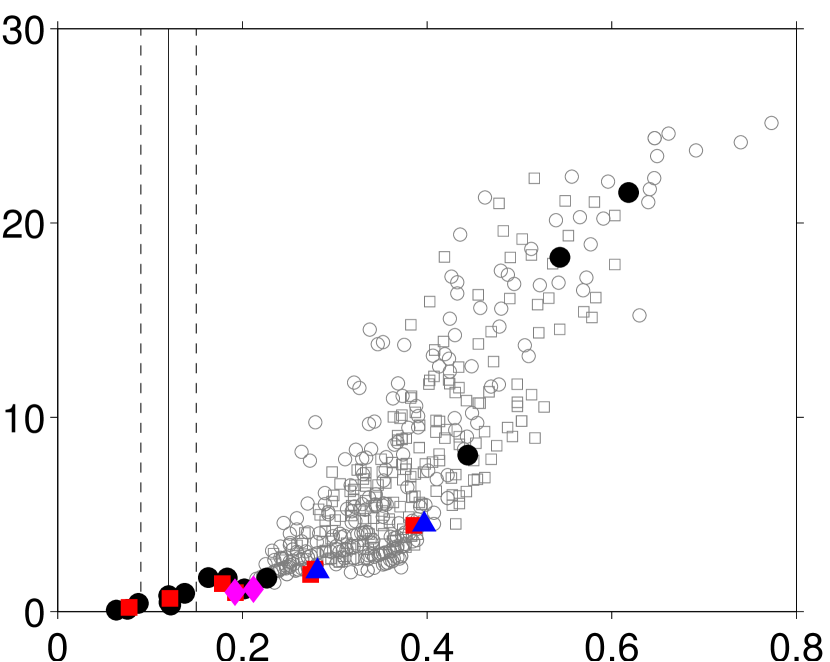
$\Theta_{Pois}$

$h_{m}/D$

$h_{m}/h_{f}$

           $(b)$

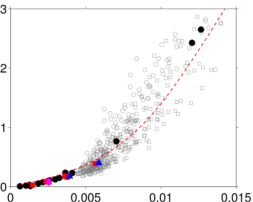
$q_{f}/q_{visc,h}$

Figure 10: Thickness of the mobile bed layer $h_{m}$: ($a$) normalized by the particle diameter $D$ and given as a function of the Shields number $\Theta_{Pois}$; ($b$) normalized by the fluid height $h_{f}$ and given as a function of the non-dimensional fluid flux $q_{f}/q_{visc,h}$. The insets show the same data in logarithmic scale. The chain-dotted lines indicate the following data fits: $(a)$ $h_{m}/D=38.01\,\Theta_{Pois}^{2.03}$; $(b)$ $h_{m}/h_{f}=12096\,(q_{f}/q_{visc,h})^{1.97}$. Data points marked by (${{{\circ}}}$,${\square}$) correspond to the experiment of Aussillous et al. (2013). In $(b)$ the dashed red line indicates the results obtained with a two-fluid model including a shear-rate dependent friction coefficient (black dashed line in figure 6$b$ of Aussillous et al., 2013).

4.2.3 Thickness of the mobile sediment bed

In practical applications involving bedload transport it is often of interest to predict the extent of the layer of particles which exhibits significant streamwise motion. Referring to the schematic of the configuration shown in figure 5, we define the thickness of the mobile layer $h_{m}$ as the distance between the fluid-bed interface location ($y_{0}$) and the location inside the bed where the mean particle velocity $\langle u_{p}\rangle$ is equal to a prescribed threshold value $\langle u_{p}\rangle^{thresh}$. In the present work we set this threshold velocity to $\langle u_{p}\rangle^{thresh}=0.005\,\max\langle u_{f}\rangle$. In terms of the Stokes settling velocity, the chosen value ranges from $0.01U_{s}$ to $0.09U_{s}$ in the different cases which we have simulated. In the study of Aussillous et al. (2013) the mobile layer thickness $h_{m}$ has been determined by a similar thresholding criterion.

Figure 10($a$) shows the computed mobile layer thickness $h_{m}$ normalized by the diameter of the particles as a function of the Shields number; figure 10($b$) shows the same quantity under the alternative normalization with the fluid height, plotted as a function of the non-dimensional fluid flow rate. Once again, the DNS data shows very good agreement with the experimental data despite the sensitivity of this quantity due to thresholding. The data in figure 10 clearly shows that $h_{m}$ monotonically increases with increasing values of the Shields number and with the non-dimensional fluid flow rate. It can be observed that the DNS-DEM data over the presently investigated parameter range is fairly well represented by a quadratic law in both graphs. This result is in contrast to some of the available models in the literature. Mouilleron et al. (2009) have considered the viscous re-suspension theory of Leighton and Acrivos (1986) in which particles are assumed to have no inertia and a mass balance between downward sedimentation and upward diffusion is considered. Ouriemi et al. (2009) on the other hand consider a continuum description of the problem where a frictional rheology (using a Coulomb model with a constant friction coefficient) is assumed to describe the mobile granular layer. In both theoretical approaches (Mouilleron et al., 2009; Ouriemi et al., 2009) the authors arrive at a linear variation of the thickness of the mobile layer with the Shields number. More recently, Aussillous et al. (2013) have essentially revisited the two-fluid modelling approach of Ouriemi et al. (2009), but employing more sophisticated closures for the stress tensor of the particle phase. In particular, they use a granular frictional rheology with a shear-rate dependent friction coefficient. These authors’ results for the mobile layer thickness obtained with this continuum approach are included in figure 10$(b)$. It can be seen that the match with our data is very reasonable at larger values of the fluid flux $q_{f}$. For smaller values of $q_{f}$ the continuum model results clearly deviate from the presently observed quadratic behavior. This, however, is not much of a surprise since the thickness of the mobile layer is very small in that range, and the continuum approach might not be appropriate. Please note, however, that the definition of the mobile layer thickness in the continuum model context is not identical to the definition which is employed in both the present work and in the experiment (Aussillous et al., 2013).

Going back to the present simulation data, it can be seen that at larger values of the two alternative control parameters our results are in fact not inconsistent with a linear variation of the mobile layer thickness with both Shields number (figure 10$a$) and with the fluid flow rate (figure 10$b$). However, in view of the fact that the data points (both in the experiment and in the simulation) cover only a limited range of these control parameters, and considering the scatter of the experimental data, this issue cannot be settled at the present time.

$(a)$

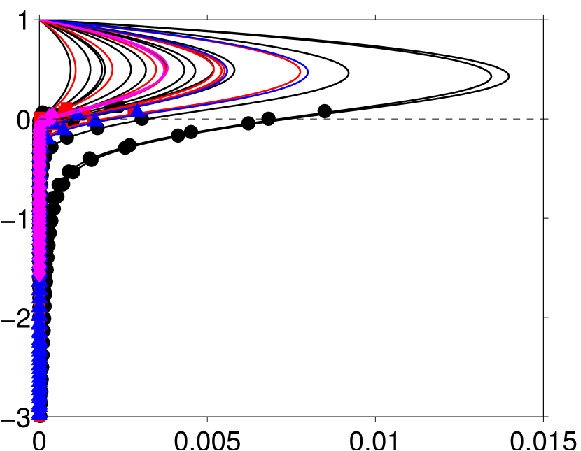
$[\langle u_{f}\rangle,\langle u_{p}\rangle]h_{f}/q_{visc,h}$

$(y-y_{0})/h_{f}$

$(y-y_{0}+h_{m})/h_{f}$

$(b)$

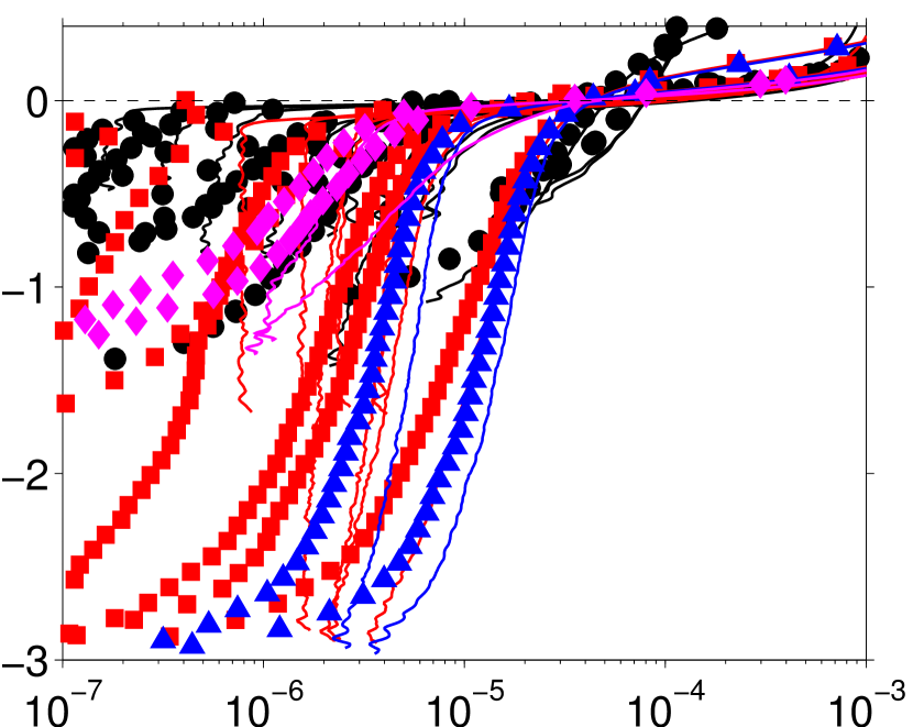
$[\langle u_{f}\rangle,\langle u_{p}\rangle]h_{f}/q_{visc,h}$

Figure 11: Wall-normal profiles of the streamwise component of the mean fluid velocity $\langle u_{f}\rangle$ (solid lines) and of the mean particle velocity $\langle u_{p}\rangle$ (symbols); color and symbol coding as indicated in table 4. In $(a)$ the ordinate is shifted to the fluid-bed interface location, while in $(b)$ it is shifted to the lower boundary of the mobile layer.

4.2.4 Fluid and particle velocities

The wall-normal profiles of the streamwise component of the mean fluid and particle velocities $\langle u_{f}\rangle$ and $\langle u_{p}\rangle$ for all cases are shown in figure 11. In this figure the length and velocity scales proposed by Aussillous et al. (2013) ($h_{f}$ and $q_{visc,h}/h_{f}$, respectively) are used. The graph in figure 11$(a)$ features an ordinate which is shifted to the fluid-bed interface location ($y_{0}$), while in figure 11$(b)$ the location of the bottom of the mobile layer ($y_{0}-h_{m}$) is used as the zero of the ordinate. Similar to what has been observed in the experiments (Aussillous et al., 2013), the present profiles exhibit three distinct regions: (I) the clear fluid region ($0<y-y_{0}<h_{f}$), where the mean fluid velocity profile is characterized by a near-parabolic shape, while the solid volume fraction is negligibly small; (II) the mobile granular layer ($-h_{m}<y-y_{0}<0$), where both the fluid and particles are in motion; (III) the bottom region ($y<y_{0}-h_{m}$), where the velocities of both phases are vanishingly small. It can be observed from figure 11 that there exists no significant difference between the mean velocities of the two phases. Note that in the clear fluid region (I) particles are occasionally entrained into the bulk flow, reaching larger distances above the mobile layer. However, the mean particle velocity at these points was not determined with sufficient statistical accuracy, and these values are, therefore, not shown in figure 11.

$(a)$

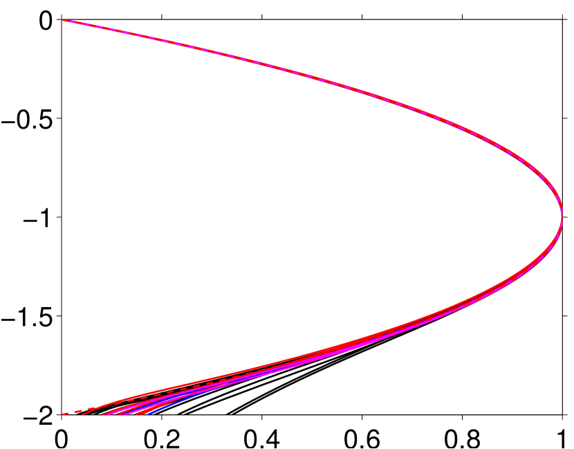
$\langle u_{f}\rangle/U_{f}^{m}$

$\tilde{y}/h^{*}$

$U_{f}^{m}h_{f}/q_{visc,h}$

$(b)$

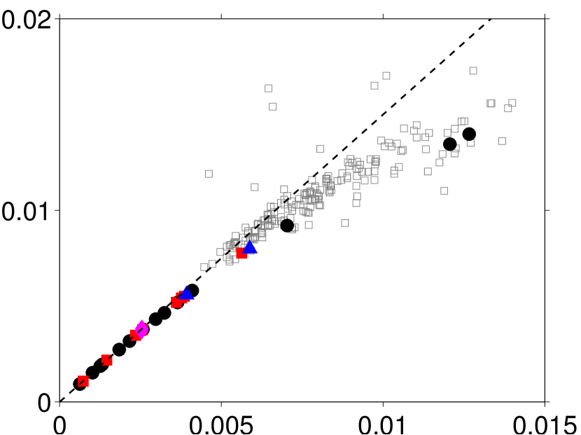
$q_{f}/q_{visc,h}$

$h^{*}/h_{f}$

$(c)$

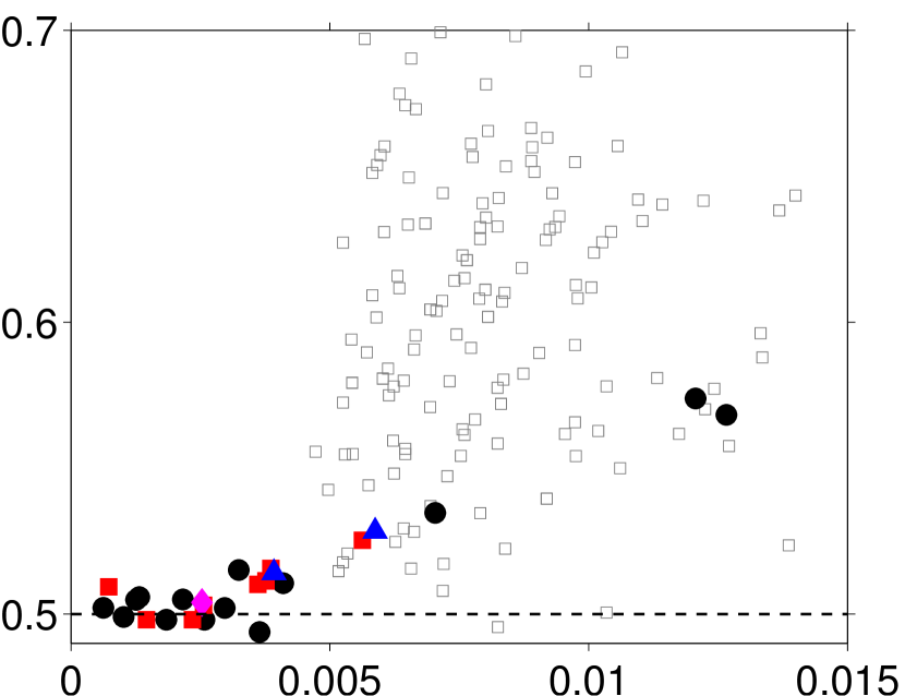
$q_{f}/q_{visc,h}$

Figure 12: ($a$) Wall-normal profile of the fluid velocity $\langle u_{f}\rangle$  normalized by its maximum value $U_{f}^{m}$. The vertical axis corresponds to $\tilde{y}=y-L_{y}$, scaled by the wall-normal distance $h^{*}$ between the top upper wall and the location of the maximum velocity $U_{f}^{m}$. The red dashed curve corresponds to the Poiseuille flow parabola (31). ($b$) The variation of $U_{f}^{m}$ as a function of $q_{f}$. The dashed line corresponds to the value for smooth wall Poiseulle flow, i.e. $(3/2)q_{f}/h_{f}$. ($c$) The variation of $h^{*}$as a function of $q_{f}$ with the Pouiseuille value $h^{*}/h_{f}=1/2$ marked by a dashed line. Data points marked by (${{{\circ}}}$,${\square}$) correspond to the experiment of Aussillous et al. (2013).

In the laminar flow regime the fluid velocity profile in the clear fluid region of the channel would be exactly of parabolic shape if that region were strictly devoid of particles. Deviations from the parabola are investigated in figure 12. For this purpose we normalize the mean particle velocity $\langle u_{f}\rangle(y)$ by its respective maximum value $U_{f}^{m}=\max\langle u_{f}\rangle$, and define a coordinate measuring the distance from the top wall, $\tilde{y}=y-L_{y}$. We also denote by $h^{*}$ the distance of the location of $U_{f}^{m}$ measured from the top wall (cf. the schematic diagram in figure 5). Figure 12($a$) shows a graph of $\langle u_{f}\rangle$ under this scaling. It can be seen that all cases collapse upon the Poiseuille flow parabola,

$$\frac{\langle u_{f}\rangle}{U_{f}^{m}}=-\Big{(}\frac{\tilde{y}}{h^{*}}\Big{)}^{2}-2\Big{(}\frac{\tilde{y}}{h^{*}}\Big{)}\;,$$ (31)

over a large wall-normal interval. Deviations from the parabolic shape are noticeable for $y\leq y_{0}$, which is a case dependent location under the scaling of figure 12($a$). These deviations are of the form of larger velocity values than those given by (31) around the fluid-bed interface. Note that in a smooth wall laminar Poiseuille flow we have $h^{*}=h_{f}/2$ and $q_{f}=2U_{f}^{m}h_{f}/3$. Thus the dependence of the characteristics of the fluid velocity profile on the non-dimensional fluid flow rate can be inferred by examining the variation of $U_{f}^{m}h_{f}/q_{visc,h}$ and $h^{*}/h_{f}$ as a function of $q_{f}/q_{visc,h}$. These quantities are shown in figure 12($b$) and 12($c$). It is seen that, for values of $q_{f}/q_{visc,h}$ smaller than approximately $0.004$, the profiles seem to be adequately described by smooth wall Poiseuille flow. At larger values of the non-dimensional flow rate, however, $U_{f}^{m}$ is observed to deviate progressively from the Poiseuille values, exhibiting an increasingly smaller slope. The opposite trend is found for $h^{*}$, which grows beyond the Poiseuille flow value with increasing $q_{f}/q_{visc,h}$. Figure 12$(b,c)$ also includes corresponding values computed from the available experimental data of Aussillous et al. (2013). Despite some scatter in the values from the experiments, a very good match with the simulation data is obtained for $U_{f}^{m}$. On the other hand, the experimental values of $h^{*}$ are highly scattered, making a direct comparison difficult.

5 Conclusion

In the present work we have performed direct numerical simulation of horizontal channel flow over a thick bed of mobile sediment particles. For this purpose we have employed an existing fluid solver which features an immersed boundary technique for the efficient and accurate treatment of the moving fluid-solid interfaces. The algorithm was coupled with a collision model based upon the soft-sphere approach. The forces arising during solid-solid contact are expressed as a function of the overlap length, with an elastic and a damping normal force component, as well as a damping tangential force, limited by a Coulomb friction law. Since the characteristic collision time is typically orders of magnitude smaller than the time step of the flow solver, the numerical integration of the equations for the particle motion is carried out with the aid of a sub-stepping technique, essentially freezing the hydrodynamic forces acting upon the particles in the interval between successive flow field updates.

The collision strategy was validated with respect to the test case of gravity-driven motion of a single sphere colliding with a horizontally oriented plane wall in a viscous fluid. Simulations over a range of collisional Stokes numbers corresponding to roughly three orders of magnitude have been performed. It was found that the present collision strategy works correctly when coupled to the particulate flow solver, yielding values for the effective coefficient of restitution in close agreement with reference data from experimental measurements.

We have then presented a series of fully-resolved simulations of bedload transport by laminar flow in a plane channel configuration similar to the experiment of Aussillous et al. (2013). Although the Reynolds number in the simulations is two orders of magnitude larger than in the experiment, the range of values of the principal control parameters of the problem (either the Shields number or the non-dimensional flow rate) overlaps significantly between both approaches, allowing for a direct comparison. Our DNS-DEM method was found to provide results which are fully consistent with the available data from the reference experiment. The present simulations yield a cubic variation of the particle flow rate (normalized by the square of the Galileo number times viscosity) with the Shields number, once the threshold value of the Shields number is exceeded. The thickness of the mobile particle layer (normalized with the particle diameter) obtained from our simulations varies roughly with the square of the Shields number; when normalized with the height of the fluid layer, it follows even more closely a quadratic variation with the normalized fluid flow rate. Previous studies using two-fluid models have predicted a linear dependency of the mobile layer thickness on both parameters (Mouilleron et al., 2009; Ouriemi et al., 2009). Unfortunately, the data for this quantity extracted from the experiment of Aussillous et al. (2013) features a certain amount of scatter, and, therefore, it does not serve to clearly distinguish between the two power laws. Based upon the DNS-DEM results we were also able to show that the deviation from a parabolic flow profile in the clear fluid region above the bed begins to become significant for non-dimensional flow rates above a value of approximately $0.004$.

The present work shows that the simple collision model considered herein is adequate for the purpose of simulating fluid-induced transport of a dense bed of spherical particles. This conclusion opens up the possibility to apply the present technique to the problem of the formation of sediment patterns (such as dunes) in wall-bounded shear flow. Another future perspective is to extend the investigation of the bedload problem itself. It bears a number of open questions, such as the lack of a precise description of the local balance of forces acting on the particles as well as a missing analysis of the Lagrangian aspects of the particle motion, which could be addressed with the aid of the present methodology.

Acknowledgments

Thanks is due to Pascale Aussillous and Élisabeth Guazzelli for sharing their data in electronic form and for fruitful discussions throughout this work. AGK acknowledges the hospitality of the group “GEP” at IUSTI, Polytech Marseille, during an extended stay. This work was supported by the German Research Foundation (DFG) through grant UH 242/2-1. The computer resources, technical expertise and assistance provided by the staff at LRZ München (grant pr58do) are thankfully acknowledged.

Appendix A Supplementary material

Animations of the particle motion in the simulations of § 4 can be found in the online version at 10.1016/j.ijmultiphaseflow.2014.08.008. The data is also available under the following URL: http://www.ifh.kit.edu/dns_data/particles/bedload.

Appendix B Averaging operations

B.1 Wall-parallel plane and time averaging

Let us first define an indicator function $\phi_{f}(\mathbf{x},t)$ for the fluid phase which tells us whether a given point with a position vector $\mathbf{x}$ lies inside $\Omega_{f}(t)$, the part of the computational domain $\Omega$ which is occupied by the fluid at time $t$, as follows:

$$\phi_{f}(\mathbf{x},t)=\left\{\begin{array}[]{lll}1&\mbox{if}&\mathbf{x}\in\Omega_{f}(t)\\ 0&\mbox{else}&\end{array}\right.\,.$$ (32)

The solid-phase indicator function $\phi_{\mathrm{p}}$ is then simply given as the complement of $\phi_{\mathrm{f}}$, i.e.

$$\phi_{\mathrm{p}}(\mathbf{x},t)=1-\phi_{\mathrm{f}}(\mathbf{x},t).$$ (33)

Based upon the indicator function $\phi_{f}$, an instantaneous discrete counter of fluid sample points in a wall-parallel plane at a given wall-distance $y_{j}$ at time $t^{m}$ is defined as:

$$n_{xz}(y_{j},t^{m})=\sum_{i=1}^{N_{x}}\sum_{k=1}^{N_{z}}\phi_{f}(\mathbf{x}_{ijk},t^{m})\,,$$ (34)

where $N_{x}$ and $N_{z}$ are the number of grid nodes in the streamwise and spanwise directions, and $\mathbf{x}_{ijk}=(x_{i},y_{j},z_{k})^{T}$ denotes a discrete grid position. The corresponding counter accounting for $N_{t}$ time records is defined as:

$$n(y_{j})=\sum_{m=1}^{N_{t}}n_{xz}(y_{j},t^{m})\,.$$ (35)

Consequently, the ensemble average of a Eulerian quantity $\boldsymbol{\xi}_{f}$ of the fluid phase over wall-parallel planes (considering only grid points located in the fluid domain) is defined as:

$$\langle\boldsymbol{\xi}_{f}\rangle_{xz}(y_{j},t^{m}) = \frac{1}{n_{xz}(y_{j},t^{m})}\sum_{i=1}^{N_{x}}\sum_{k=1}^{N_{z}}\phi_{f}(\mathbf{x}_{ijk},t^{m})\,\boldsymbol{\xi}_{f}(\mathbf{x}_{ijk},t^{m})$$ (36)

$$\langle\boldsymbol{\xi}_{f}\rangle(y_{j}) = \frac{1}{n(y_{j})}\sum_{m=1}^{N_{t}}n_{xz}(y_{j},t^{m})\langle\boldsymbol{\xi}_{f}\rangle_{xz}(y_{j},t^{m})\,,$$ (37)

where the operator $\langle\cdot\rangle_{xz}$ indicates an instantaneous spatial wall-parallel plane average and $\langle\cdot\rangle$ indicates an average over space and time.

B.2 Binned averages over particle-related quantities

Concerning Eulerian statistics of (Lagrangian) particle-related quantities, the computational domain was decomposed into discrete wall-parallel bins of thickness $\Delta h$, and averaging was performed over all those particles within each bin. Similar to (32), we define an indicator function $\phi_{bin}^{(j)}(y)$ which tells us whether a given wall-normal position $y$ is located inside or outside a particular bin with index $j$, viz.

$$\phi_{bin}^{(j)}(y)=\left\{\begin{array}[]{lll}1&\mbox{if}&(j-1)\Delta h\leq y<j\Delta h\\ 0&\mbox{else}\;.&\end{array}\right.$$ (38)

A sample counter for each bin, sampled over an instantaneous time $t^{m}$ as well as sampled over the number of available snapshots of the solid phase, $N_{t}^{(p)}$, is defined as

$$n_{p_{xz}}^{(j)}(t^{m}) = \sum_{l=1}^{N_{p}}\phi_{bin}^{(j)}(y_{p}^{(l)}(t^{m}))\,,$$ (39)

$$n_{p}^{(j)} = \sum_{m=1}^{N_{t}^{(p)}}n_{p_{xz}}^{(j)}(t^{m})\,,$$ (40)

respectively. From the sample counters we can deduce the (instantaneous) average solid volume fraction in each bin, viz.

$$\langle\phi_{s}\rangle_{xz}(y^{(j)},t^{m}) = n_{p_{xz}}^{(j)}(t^{m})\frac{\pi D^{3}}{6L_{x}L_{z}\Delta h}\,,$$ (41)

$$\langle\phi_{s}\rangle(y^{(j)}) = \frac{n_{p}^{(j)}}{N_{t}^{(p)}}\,\frac{\pi D^{3}}{6L_{x}L_{z}\Delta h}\,.$$ (42)

Alternatively, the solid volume fraction can be deduced from the indicator function defined in (32) viz.

$$\langle\phi_{p}\rangle_{zt}(x_{i},y_{j}) = \frac{1}{N_{t}^{(p)}N_{z}}\sum_{m=1}^{N_{t}^{(p)}}\sum_{k=1}^{N_{z}}\big{(}1-\phi_{f}(\mathbf{x}_{ijk},t^{m})\big{)}\,,$$ (43)

$$\langle\phi_{p}\rangle(y_{j}) = \frac{1}{N_{x}}\sum_{k=1}^{N_{x}}\langle\phi_{p}\rangle_{zt}(x_{i},y_{j})\,,$$ (44)

where the operator $\langle\cdot\rangle_{zt}$ indicates averaging in the spanwise direction and time, and $\langle\cdot\rangle$ indicates an average over both homogeneous directions and time. Finally, the binned average of a Lagrangian quantity $\boldsymbol{\xi}_{p}$ is defined as follows:

$$\langle\boldsymbol{\xi}_{p}\rangle_{xz}(y^{(j)},t^{m}) = \frac{1}{n_{p_{xz}}^{(j)}(t^{m})}\sum_{l=1}^{N_{p}}\phi_{bin}^{(j)}(y_{p}^{(l)}(t^{m}))\,\boldsymbol{\xi}_{p}^{(l)}(t^{m})\,,$$ (45)

$$\langle\boldsymbol{\xi}_{p}\rangle(y^{(j)}) = \frac{1}{n_{p}^{(j)}}\sum_{m=1}^{N_{t}^{(p)}}n_{p_{xz}}^{(j)}(t^{m})\langle\boldsymbol{\xi}_{p}\rangle_{xz}(y^{(j)},t^{m})\,,$$ (46)

supposing that a finite number of samples has been encountered ($n_{p_{xz}}^{(j)}(t^{m})>0$, $n_{p}^{(j)}>0$). A bin thickness of $\Delta h=D/4$ was chosen for the evaluation of the binned averages, unless otherwise stated.

References

- Aussillous et al. (2013) Aussillous, P., Chauchat, J., Pailha, M., Médale, M., Guazzelli, E., 2013. Investigation of the mobile granular layer in bedload transport by laminar shearing flows. J. Fluid Mech. 736, 594--615.
- Boyer et al. (2011) Boyer, F., Guazzelli, E., Pouliquen, O., 2011. Unifying suspension and granular rheology. Phys. Rev. Lett. 107, 188301.
- Brändle de Motta et al. (2013) Brändle de Motta, J.C., Breugem, W.P., Gazanion, B., Estivalezes, J.L., Vincent, S., Climent, E., 2013. Numerical modelling of finite-size particle collisions in a viscous fluid. Phys. Fluids 25, 083302.
- ten Cate et al. (2002) ten Cate, A., Nieuwstad, C.H., Derksen, J.J., Van den Akker, H.E.A., 2002. Particle imaging velocimetry experiments and lattice-Boltzmann simulations on a single sphere settling under gravity. Phys. Fluids 14, 4012.
- Chan-Braun et al. (2011) Chan-Braun, C., García-Villalba, M., Uhlmann, M., 2011. Force and torque acting on particles in a transitionally rough open-channel flow. J. Fluid Mech. 684, 441--474.
- Charru et al. (2007) Charru, F., Larrieu, E., Dupont, J.B., Zenit, R., 2007. Motion of a particle near a rough wall in a viscous shear flow. J. Fluid Mech. 570, 431.
- Charru et al. (2004) Charru, F., Mouilleron, H., Eiff, O., 2004. Erosion and deposition of particles on a bed sheared by a viscous flow. J. Fluid Mech. 519, 55--80.
- Charru and Mouilleron-Arnould (2002) Charru, F., Mouilleron-Arnould, H., 2002. Instability of a bed of particles sheared by a viscous flow. J. Fluid Mech. 452, 303--323.
- Cleary and Prakash (2004) Cleary, P.W., Prakash, M., 2004. Discrete-element modelling and smoothed particle hydrodynamics: potential in the environmental sciences. Philos. Trans. A. Math. Phys. Eng. Sci. 362, 2003--30.
- Constantinides et al. (2008) Constantinides, G., Tweedie, C., Holbrook, D., Barragan, P., Smith, J., Vliet, K.V., 2008. Quantifying deformation and energy dissipation of polymeric surfaces under localized impact. Mat. Sci. Eng. A 489, 403 -- 412.
- Crowe et al. (1998) Crowe, C., Sommerfeld, M., Tsuji, Y., 1998. Multiphase flows with droplets and particles. CRC Press.
- Cundall and Strack (1979) Cundall, P.A., Strack, O.D.L., 1979. A discrete numerical model for granular assemblies. Géotechnique 29, 47--65.
- Foerster et al. (1994) Foerster, S.F., Louge, M.Y., Chang, H., Allia, K., 1994. Measurements of the collision properties of small spheres. Phys. Fluids 6, 1108.
- García (2008) García, M.H. (Ed.), 2008. Sedimentation engineering: processes, measurements, modeling, and practice. ASCE Publications. 110 edition.
- García-Villalba et al. (2012) García-Villalba, M., Kidanemariam, A.G., Uhlmann, M., 2012. DNS of vertical plane channel flow with finite-size particles: Voronoi analysis, acceleration statistics and particle-conditioned averaging. Int. J. Multiph. Flow 46, 54--74.
- Glowinski et al. (1999) Glowinski, R., Pan, R., Hesla, T.I., Joseph, D.D., 1999. A distributed Lagrange multiplier/fictitious domain method for particulate flows. Int. J. Multiph. Flow 25, 755--794.
- Gondret et al. (2002) Gondret, P., Lance, M., Petit, L., 2002. Bouncing motion of spherical particles in fluids. Phys. Fluids 14, 643--652.
- Heald et al. (2004) Heald, J., McEwan, I., Tait, S., 2004. Sediment transport over a flat bed in a unidirectional flow: simulations and validation. Philos. Trans. A. Math. Phys. Eng. Sci. 362, 1973--86.
- Joseph and Hunt (2004) Joseph, G.G., Hunt, M.L., 2004. Oblique particle-wall collisions in a liquid. J. Fluid Mech. 510, 71--93.
- Joseph et al. (2001) Joseph, G.G., Zenit, R., Hunt, M.L., Rosenwinkel, A.M., 2001. Particle-wall collisions in a viscous fluid. J. Fluid Mech. 433, 329--346.
- Kempe and Fröhlich (2012) Kempe, T., Fröhlich, J., 2012. Collision modelling for the interface-resolved simulation of spherical particles in viscous fluids. J. Fluid Mech. 709, 445--489.
- Kidanemariam et al. (2013) Kidanemariam, A.G., Chan-Braun, C., Doychev, T., Uhlmann, M., 2013. Direct numerical simulation of horizontal open channel flow with finite-size, heavy particles at low solid volume fraction. New J. Phys. 15, 025031.
- Leighton and Acrivos (1986) Leighton, D., Acrivos, A., 1986. Viscous resuspension. Chem. Eng. Sci. 41, 1377--1384.
- Li et al. (2011) Li, X., Hunt, M.L., Colonius, T., 2011. A contact model for normal immersed collisions between a particle and a wall. J. Fluid Mech. 691, 123--145.
- Lobkovsky et al. (2008) Lobkovsky, A.E., Orpe, A.V., Molloy, R., Kudrolli, A., Rothman, D.H., 2008. Erosion of a granular bed driven by laminar fluid flow. J. Fluid Mech. 605, 47--58.
- Loiseleux et al. (2005) Loiseleux, T., Gondret, P., Rabaud, M., Doppler, D., 2005. Onset of erosion and avalanche for an inclined granular bed sheared by a continuous laminar flow. Phys. Fluids 17, 103304.
- Mouilleron et al. (2009) Mouilleron, H., Charru, F., Eiff, O., 2009. Inside the moving layer of a sheared granular bed. J. Fluid Mech. 628, 229.
- Nguyen and Ladd (2002) Nguyen, N., Ladd, A., 2002. Lubrication corrections for lattice-Boltzmann simulations of particle suspensions. Phys. Rev. E 66, 046708.
- Ouriemi et al. (2009) Ouriemi, M., Aussillous, P., Guazzelli, E., 2009. Sediment dynamics. Part 1. Bed-load transport by laminar shearing flows. J. Fluid Mech. 636, 295--319.
- Ouriemi et al. (2007) Ouriemi, M., Aussillous, P., Medale, M., Peysson, Y., Guazzelli, E., 2007. Determination of the critical Shields number for particle erosion in laminar flow. Phys. Fluids 19, 061706.
- Patankar and Joseph (2001) Patankar, N., Joseph, D., 2001. Modeling and numerical simulation of particulate flows by theEulerian-Lagrangian approach. Int. J. Multiphase Flow 27, 1659--1684.
- Schmeeckle and Nelson (2003) Schmeeckle, M.W., Nelson, J.M., 2003. Direct numerical simulation of bedload transport using a local, dynamic boundary condition. Sedimentology , 279--301.
- Shields (1936) Shields, A., 1936. Anwendung der Ähnlichkeitsmechanik und der Turbulenzforschung auf die Geschiebebewegung. Mitteilungen der Versuchanstalt für Wasserbau und Schiffbau. Technischen Hochschule Berlin.
- Silbert et al. (2001) Silbert, L., Ertaş, D., Grest, G., Halsey, T., Levine, D., Plimpton, S., 2001. Granular flow down an inclined plane: Bagnold scaling and rheology. Phys. Rev. E 64, 051302.
- Simeonov and Calantoni (2012) Simeonov, J.A., Calantoni, J., 2012. Modeling mechanical contact and lubrication in Direct Numerical Simulations of colliding particles. Int. J. Multiph. Flow 46, 38--53.
- Tsuji et al. (1993) Tsuji, Y., Kawaguchi, T., Tanaka, T., 1993. Discrete particle simulation of two-dimensional fluidized bed. Powder Technol. 77, 79--87.
- Uhlmann (2004) Uhlmann, M., 2004. New Results on the Simulation of Particulate Flows. Technical Report. CIEMAT. Madrid.
- Uhlmann (2005a) Uhlmann, M., 2005a. An immersed boundary method with direct forcing for the simulation of particulate flows. J. Comput. Phys. 209, 448--476.
- Uhlmann (2005b) Uhlmann, M., 2005b. An improved fluid-solid coupling method for DNS of particulate flow on a fixed mesh, in: Sommerfel, M. (Ed.), Proc. 11th Work. Two-Phase Flow Predict., Universität Halle, Merseburg, Germany.
- Uhlmann (2006) Uhlmann, M., 2006. Experience with DNS of particulate flow using a variant of the immersed boundary method, in: Wesseling, P., Onate, E., Périaux, J. (Eds.), Proc. ECCOMAS CFD 2006, TU Delft, Egmond aan Zee, The Netherlands.
- Uhlmann (2008) Uhlmann, M., 2008. Interface-resolved direct numerical simulation of vertical particulate channel flow in the turbulent regime. Phys. Fluids 20, 053305.
- Uhlmann and Dušek (2014) Uhlmann, M., Dušek, J., 2014. The motion of a single heavy sphere in ambient fluid: a benchmark for interface-resolved particulate flow simulations with significant relative velocities. Int. J. Multiphase Flow 59, 221--243.
- Wachs (2009) Wachs, A., 2009. A DEM-DLM/FD method for direct numerical simulation of particulate flows: Sedimentation of polygonal isometric particles in a Newtonian fluid with collisions. Comput. Fluids 38, 1608--1628.
- Yang and Hunt (2006) Yang, F.L., Hunt, M.L., 2006. Dynamics of particle-particle collisions in a viscous liquid. Phys. Fluids 18, 121506.
- Yang and Hunt (2008) Yang, F.L., Hunt, M.L., 2008. A mixed contact model for an immersed collision between two solid surfaces. Philos. Trans. A. Math. Phys. Eng. Sci. 366, 2205--18.