Quantum bright solitons in the Bose-Hubbard model
with site-dependent repulsive interactions

Abstract

We introduce a one-dimensional (1D) spatially inhomogeneous Bose-Hubbard model (BHM) with the strength of the onsite repulsive interactions growing, with the discrete coordinate $z_{j}$, as $|z_{j}|^{\alpha}$ with $\alpha>0$ . Recently, the analysis of the mean-field (MF) counterpart of this system has demonstrated self-trapping of robust unstaggered discrete solitons, under condition $\alpha>1$. Using the numerically implemented method of the density matrix renormalization group (DMRG), we demonstrate that, in a certain range of the interaction, the BHM also features self-trapping of the ground state into a soliton-like configuration, at $\alpha>1$, and remains weakly localized at $\alpha<1$. An essential quantum feature found in the BHM is a residual quasi-constant density of the background surrounding the soliton-like peak in the ground state, while in the MF limit the finite-density background is absent. Very strong onsite repulsion eventually destroys soliton-like states, driving the system, at integer densities, into the Mott phase with a spatially uniform density

I Introduction

The Bose-Hubbard Model (BHM), introduced in 1989 fisher as an example of a system exhibiting a quantum phase transition, has drawn a great deal of interest – in particular, due to its experimentally realizability in ultra-cold Bose gases bloch , admitting precise control of interaction terms bloch_review , and availability of probing techniques which can be applied to this system greiner ; in-situ . At the same time, BHM is the ideal platform to study exotic phenomena in reduced dimensions, where quantum fluctuations can give rise to nontrivial effects giamarchi ; cazalilla2011 .

Discrete systems with repulsive interactions, which are described by the BHM or, in the mean-field (MF) approximation, by the discrete nonlinear Schrödinger equation (DNLSE), give rise, respectively, to quantum quant-dark-sol or semi-classical dark-sol dark solitons. In the case of weak on-site attractive interactions, the kinetic energy prevents the collapse, and the system self-traps into bright solitons Salerno ; salasnich . The existence of bright solitons in an attractive Bose gas was experimentally proved in several experiments exp-solo1 ; exp-solo2 ; exp-solo3 ; exp-solo4 ; exp-solo5 . Furthermore, it was also demonstrated that repulsive interactions between atoms trapped in an optical-lattice (OL) potential give rise to gap solitons gap-sol ; morsch , which is another variety of bright modes.

At the mean-field (MF) level, it has been recently shown that, in both continuum Barcelona0 ; Barcelona and discrete boris settings, repulsive interactions with the strength growing from the center to periphery faster than $r^{D}$, where $r$ is the distance from the center and $D$ the spatial dimension, give rise to robust bright soliton-like states. Because, as is well known salasnich ; haus ; drummond ; castin ; weiss ; weiss2 ; delande ; weiss3 , the MF approximation does not provide for a full description of physical systems, in this paper we introduce the quantum BHM with the onsite repulsive interaction growing from the center to periphery. By means of the density-matrix-renormalization group (DMRG) technique white , we obtain quasi-exact results for quantum multi-boson bound states, and compare them to the MF prediction boris for self-trapped bright discrete solitons in the zero-temperature model for bosons loaded in a one-dimensional (1D) OL in the presence of the spatially modulated repulsive interactions.

The rest of the paper is organized as follows. The model is formulated in Section II. Numerical results for quantum bound states and their comparison with the MF counterparts are presented in Section III. It is found that quantum effects, which the MF approximation cannot grasp, are responsible for a discrepancy between soliton-like modes in the MF and BHM settings. At the end of Section III, we study the system in the regime of very strong self-repulsive interactions. We find that the strong repulsion destroys self-localized modes, which are replaced by states with a spatially uniform density. Those states are actually equivalent to well-known Mott insulating phase in the homogeneous BHM.

II The model

II.1 The general approach

We consider a dilute ultracold gas of bosonic atoms confined in the $(x,y)$ plane by the strong transverse harmonic potential,

$$U(x,y)=\left(m\omega_{\bot}^{2}/2\right)\left(x^{2}+y^{2}\right),$$ (1)

under the simultaneous action of the OL axial potential morsch ; book-lattice ,

$$V(z)=V_{0}\ \cos^{2}{(2k_{0}z)}\;.$$ (2)

As usual, we focus on the case of the tight transverse confinement, $V_{0}\ll\hbar\omega_{\bot}$, which implies a nearly-1D configuration. We choose the characteristic length of the transverse confinement, $a_{\bot}=\sqrt{\hbar/(m\omega_{\bot})}$, and $\hbar\omega_{\bot}$ as length and energy units, respectively, using accordingly scaled variables below. The system is described by the quantum-field-theory Hamiltonian,

$$H = \int d^{3}\mathbf{r}\ {\psi}^{+}(\mathbf{r})\Big{[}-{\frac{1}{2}}\nabla^{2}+U(x,y)+V(z)$$ (3)

$$+\pi g(z)\ {\psi}^{+}(\mathbf{r}){\psi}(\mathbf{r})\Big{]}{\psi}(\mathbf{r})\;,$$

where ${\psi}(\mathbf{r})$ is the bosonic field operator, and $g=2a_{s}(z)/a_{\bot}$, with $a_{s}$ the $s$-wave scattering length of the inter-atomic interactions book-bose .

Unlike previous numerous studies of similar quantum models, here, as said above, we aim to consider the setting with a $z$-dependent scattering length, $a_{s}=a_{s}(z)$, which implies $g=g(z)$, as suggested by the recent analysis of the MF model based on the DNLSE boris . The special inhomogeneity of the nonlinearity strength induces an effective nonlinear potential nlattice , alias a pseudopotential Dong . Experimentally the tunability of the magnetic Feshbach resonance (FR) Roati ; Pollack allows the creation of such a spatially inhomogeneous nonlinearity landscapes by means of properly shaped magnetic fields Boris1 . Furthermore, optically controlled FR Gora , as well as combined magneto-optical control mechanisms Durr , make it possible to create a diverse set of spatial profiles of the self-repulsive nonlinearity. In particular, the required pattern of the laser-field intensity controlling the optically induced FR can be “painted” in space, as demonstrated in Ref. Boshier .

II.2 The discretization and dimensional reduction

The presence of the deep OL potential suggests discretization of Hamiltonian (3) along the $z$ axis. To this end, we use the decomposition in the general form of book-lattice

$$\psi(\mathbf{r})=\sum_{j=1}^{L}{\phi}_{j}(x,y)\ w_{j}(z),$$ (4)

where $w_{j}(z)$ is the Wannier function maximally localized at the $j$-th local minimum of the axial periodic potential, and $\phi_{j}\left(x,y\right)$ are proportional to the ground state of the transverse potential (1),

$$\phi_{j}(x,y)={\frac{1}{\sqrt{\pi}}}\exp{\left[-\left({\frac{x^{2}+y^{2}}{2}}\right)\right]}\,{b}_{j}\;,$$ (5)

with ${b}_{j}$ representing the bosonic-field operator acting at site $j$, with $b_{0}=b_{L+1}\equiv 0$. In this work, we consider the case of an even number $L$ of the lattice sites, see Eq. (4).

Next, inserting ansatz (4) into Eq. (3), one can readily derive the effective 1D BHM Hamiltonian,

$$H=\sum_{j=1}^{L}\left[-J\,{b}_{j}^{\dagger}\left({b}_{j+1}+{b}_{j-1}\right)+{\frac{1}{2}}U_{j}{n}_{j}({n}_{j}-1)\right]\;,$$ (6)

where ${n}_{j}={b}_{j}^{\dagger}{b}_{j}$ is the on-site operator of the number of bosons, while $J$ and $U_{j}$ are the adimensional hopping (tunneling) amplitude and on-site energy, which are experimentally tunable via $V_{0}$ and $a_{s}$ bloch_review , and are given by

$$J = -\int_{-\infty}^{+\infty}w_{j+1}^{\ast}(z)\left[-{\frac{1}{2}}{\frac{\partial^{2}}{\partial z^{2}}}+V(z)\right]w_{j}(z)\ dz\;,$$ (7)

$$U_{j} = \int_{-\infty}^{+\infty}g(z)\ |w_{j}(z)|^{4}\ dz\;.$$ (8)

In the present model, the hopping energy does not depend on the site number $j$, therefore we normalize it to be $J=1$, while, on the contrary to the standard BHM, the on-site energy $U_{j}$ depends on $j$ through the inhomogeneous interaction strength, $g(z)$. In particular, choosing

$$g(z)=g_{0}|z|^{\alpha}$$ (9)

with spatial growth rate $\alpha>0$ [cf. Ref. Barcelona0 ], one has

$$U_{j}=U\ |z_{j}|^{\alpha}\;,$$ (10)

where $z_{j}\equiv j-\left(L+1\right)/2$ is the discrete axial coordinate, and $U_{j}$ attains minimum values

$$U_{\min}\equiv U_{L/2+1}=U_{L/2}=2^{-\alpha}U.$$ (11)

at two central sites of the lattice. Thus, in our model the inhomogeneous on-site energy depends on two parameters, amplitude $U$ and spatial growth rate $\alpha$.

II.3 MF (mean field) vs. DMRG (density-matrix renormalization group)

It is well known that, in 1D configurations, quantum fluctuations, which are omitted in the mean-field (MF) theory, play a significant role. Thus, in our 1D problem it is relevant to compare MF predictions with those produced by the DMRG, to conclude in what regimes the MF may give reliable results note , and to reveal essential quantum features of the ground state beyond the bounds of the validity of the MF approximation.

We follow the MF approach based on the Glauber coherent state, $|\mathrm{GCS}\rangle=|\beta_{1}\rangle\otimes...\otimes|\beta_{L}\rangle$, where $|\beta_{j}\rangle$ is defined so that $b_{j}|\beta_{j}\rangle=\beta_{j}|\beta_{j}\rangle$, with (complex) eigenvalues $\beta_{j}$ book-luca . By minimizing energy $\langle\mathrm{GCS}|H|\mathrm{GCS}\rangle$ with respect to $\beta_{j}$, one finds that complex numbers $\beta_{i}$ satisfy the stationary form of the 1D DNLSE,

$$\mu\,\beta_{i}=\epsilon_{i}\,\beta_{i}-J\,\left(\beta_{i+1}+\beta_{i-1}\right)+U_{i}|\beta_{i}|^{2}\beta_{i}\;,$$ (12)

where $\mu$ is the chemical potential, determined by the total number of atoms: $N=\sum_{j}|\beta_{j}|^{2}=\sum_{j}\langle\mathrm{GCS}|{n}_{j}|\mathrm{GCS}\rangle$. One can solve Eq. (12) numerically – in particular, with the help of the imaginary-time Crank-Nicolson predictor-corrector algorithm sala-numerics .

The DMRG accounts for the full quantum behavior of 1D lattice systems. As concerns the search for localized states, in previous works the DMRG has given strong evidences of bright-soliton states in the homogeneous BHM salasnich , spin chains manmana , and in bosonic models with nearest-neighbor interactions das , including disorder sacha . To produce accurate results by our DMRG-based computations, taking care of both the interaction with external sites in Hamiltonian (6) and the needed very large size of the underlying Hilbert space, we utilize open boundary conditions. We use a number of DMRG states $m$ up to $m=768$, performing $6$ finite-size sweeps white .

III Numerical results

III.1 Comparison of MF and DMRG results

III.1.1 The non-self-trapping case ($\alpha<1$)

As mentioned above boris , the MF predicts the existence of self-localized states (bright solitons) supported by the spatial modulation (9) with $\alpha>D$ Barcelona0 . Here, using a range of parameters similar to magnons , we aim to check these predictions in the BHM for $D=1$, by mean of the DMRG technique, and to look for new effects generated by quantum fluctuations. First, we do this for $\alpha<1$, when the self-trapping is not produced by the MF.

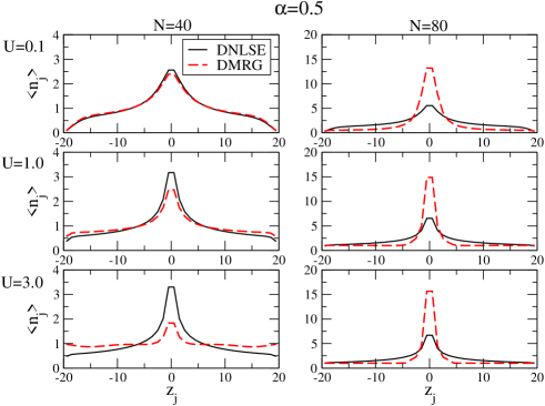
Figure 1: (Color online) DNLSE (mean-field) and DMRG density profiles, $n_{j}$, for $\alpha=0.5$, $J=1.0$ and several values of $U$ in the system with $L=40$ sites and two different values of the numbers of bosons, $N$.

In Fig. 1 we can see that, as predicted by the MF, at $\alpha=0.5$, the density profile is not self-trapped (i.e., it is not a soliton) for weak interaction $U$ and average density $n\equiv N/L=1$ (the first two panels in the left column), the MF and DMRG methods being in very good agreement. This agreement is explained by the fact that, in certain regimes, quantum fluctuations are weak and their effect is practically negligible, thus allowing semi-classical methods, such as the MF approximation, to predict the correct behavior. Non-self-trapped states are also found in the case of the weak interaction for a larger number of bosons.

On the other hand, the DMRG calculations produce sort of a bright soliton for stronger interaction (higher $U$), at average densities $n=1$ and $n=2$ alike. More precisely, the DMRG results show that a well-defined peak appears at the center of the system, surrounded by a nearly flat distribution of the bosons. Furthermore, while the shape of the density profiles produced by the MF is actually unchanged, i.e., the shape of the peak depends solely on the density, but not on the interaction strength, $U$, the DMRG-produced results do not share this feature. Indeed, for average density $n=1$, we observe that, in the DMRG states, the fraction of particles located at the center of the lattice decreases for higher $U$ and, at the same time, the number of bosons composing the background around the soliton increases. The latter feature is still more salient for higher average density, i.e. $n=2$. This effect can be explained as the possible approach of the system towards an insulating phase (the Mott phase), in a region where the interaction strength in Eq. (10) exceeds a critical value of $U$. Further details regarding this point are given below in the section addressing the Mott phase.

III.1.2 The self-trapping case ($\alpha>1$)

The MF theory predicts that spatial inhomogeneity (10) with $\alpha>D$ gives rise to self-trapping into localized states Barcelona0 ; boris . To delve deep enough in this regime, we now set $\alpha=2$.

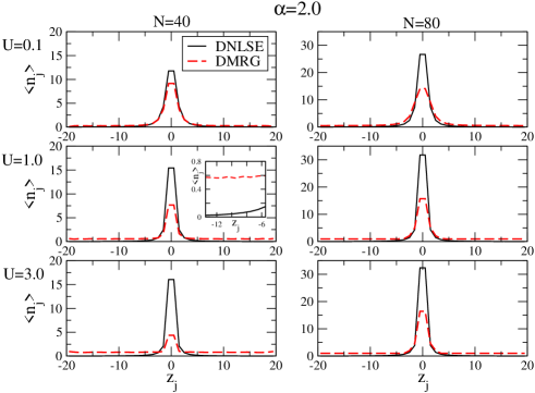
Figure 2: (Color online) DNLSE and DMRG density profiles, $n_{j}$. for $\alpha=2.0$, $J=1.0$, and several different values of $U$ in the system with $L=40$ sites and two different values of the numbers of particles, $N$. Inset: density profile $n_{j}$ at the first 10 sites of the chain, for $\alpha=2$, $J=1.0$, $N=40$ and $L=40$

In Fig. 2 it is clearly seen that the MF solutions, produced by the DNLSE, indeed yield well self-trapped states, with vanishing density around the central peak. Of course, in this case the peak is higher than at $\alpha=0.5$, because the corresponding effective interaction is much stronger in Eq. (10).

In the present case, the DMRG results also exhibit, in agreement with their MF counterparts, self-localized states. Nevertheless, a finite constant background, which is higher for larger $U$, is again observed around the quasi-soliton states. Furthermore, due to the stronger interaction, in comparison to the case of $\alpha=0.5$, the full quantum approach demonstrates a larger disagreement with MF even at $U=0.1$.

III.2 Transition from weakly localized to self-trapped states

Figures 1 and 2 clearly demonstrate that the transition from a weakly localized state to a self-trapped one is driven by the interaction strength $U$. In particular, the soliton-like state always comes with a constant finite background, while both the height and the width of the central peak depend on the interaction strength. In order to clearly define weakly and strongly localized states, in Fig 3 we plot the standard deviation relative to the external sites of the lattice,

$$\sigma=\sqrt{\frac{\sum_{j}(\langle n_{j}\rangle-\bar{n})^{2}}{\tilde{L}}}$$ (13)

where $\bar{n}$ is the average value $\langle n_{j}\rangle$ over $\tilde{L}$, which is the number of external lattice sites. In Fig. 3 it is possible to clearly identify, for all the values of $\alpha$ that we considered, two distinct regimes: one where the value of $\sigma$ changes for different $U$, meaning that there is no constant background, and another one, where $\sigma$ is insensitive to the interaction strength, signaling the appearance of a practically constant background density profile and thus revealing the presence of a soliton-like solution existing on top of the background. It is worthy to note that, for the strong interaction, a self-trapped solution is possible even for $\alpha<1$.

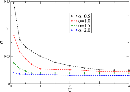
Figure 3: (Color online) DMRG results for the standard deviation $\sigma$ computed for $\tilde{L}=10$ [see Eq. (13)], in a system with $L=40$, $N=40$, $J=1.0$ and different values of $U$ and $\alpha$.

III.3 Quantum effects

The purely quantum part in interaction density, $n_{j}(n_{j}-1)$, in the BHM Hamiltonian (6) is represented by term $-1$ book-lattice . To understand if it is responsible for the appearance of the above-mentioned nonvanishing background surrounding the soliton peak in the DMRG density profiles, i.e., if this quantum term is the source of discrepancies between the MF and DMRG solutions, we have additionally performed the quasi-exact DMRG-based calculations, but in the “truncated” form, with $\left(n_{j}-1\right)$ replaced by $n_{j}$ in Eq. (6).

Figure 4: (Color online) The DNLSE and “truncated-DMRG” density profiles, $n_{j}$ (without the quantum term $-1$ term in the latter case, see the text). Upper panel: $\alpha=2$, $J=1.0$ and $U=3.0$ in the system with $L=40$ sites and $N=40$ particles. Lower panel: $\alpha=0.5$, $J=1.0$ and $U=3.0$ in the system with $L=40$ sites and $N=40$ particles.

In Fig 4 we compare the MF and the truncated-DMRG profiles, for two different values of $\alpha$, with average density $n=1$ and $U=3.0$. As shown above in Figs. 1 and 2, the MF and normal DMRG methods are strongly discordant at these values of the parameters. Here we see that, without the above-mentioned $-1$ term, the finite background around the peak disappears in the truncated-DMRG state, making it perfectly similar to the MF counterpart at $\alpha=2$. At $\alpha=0.5$, when non-self-trapped states are produced by the DNLSE, it also matches well to the truncated-DMRG counterpart, but in this case small discrepancies are still visible. Interestingly, the comparison between the lower panel in the left column of Fig. 1 and the lower panel in Fig. 4 shows that the truncated-DMRG results still produce a conspicuous self-trapped peak, whereas in the case of the full quantum description the peak is very weak. This comparison demonstrates that truly quantum ingredients of the system (as a matter of fact, quantum fluctuations) may account for peculiar effects which are not captured by the MF or nearly-MF description.

IV Transition from self-trapped states to the Mott phase

To check if self-trapped states can be always found in the true quantum system, in Fig. 5 we plot the density at the central sites, $\left\langle n_{L/2+1}\right\rangle=\left\langle n_{L/2}\right\rangle$ comment1 , for several values of the interaction strength, $U$, and spatial growth rate, $\alpha$ in Eq. (9). More precisely, we aim to find out how the variation of $U$ modifies the shape of the bosonic cloud which, as shown before, may be characterized by the density at the two central sites, where the repulsive interaction is weakest.

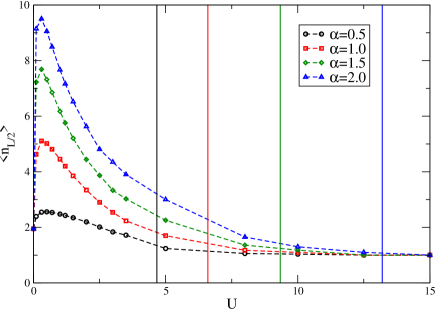
Figure 5: (Color online) DMRG results for the density at the center, $\left\langle n_{L/2}\right\rangle$, for $L=40$, $N=40$, $J=1.0$ and different values of $U$ and $\alpha$. Vertical lines correspond to the respective critical values for the Mott-superfluid transition in the finite-size homogeneous system, estimated as per Eq. (14).

Figure 5 clearly demonstrates that, at fixed $\alpha$, the height of the soliton peak in the BHM depends by $U$, on the contrary to the MF prediction. In particular for weak interactions we find a maximum in $\left\langle n_{L/2}\right\rangle$ at a certain value of $U$, which is nearly the same for all $\alpha$. Then, with the further increase of $U$, the double occupation become more energetically expensive and the number of bosons forming the soliton peak decreases, while the boson number increases in the background surrounding the peak, making the background density closer to $1$. As seen in Fig. 5, this behavior persists, at all values of $\alpha$, up to a critical point, $U=U_{c}(\alpha)$ (the critical values are represented by vertical lines in Fig. 5. At $U>U_{c}(\alpha)$, the behavior is different, featuring $\left\langle n_{L/2}\right\rangle=\left\langle n_{j}\right\rangle\equiv 1$. The latter regime means that the inhomogeneous BHM, resembling its homogeneous counterpart fisher , has entered a state with the spatially uniform boson density, which is the insulating Mott phase, where the superfluid density vanishes. It is well known that the Mott-superfluid transition in 1D is of the Kosterlitz-Thouless type sachdev , which means that the respective gap opens up exponentially, hence precise determination of the transition point requires an accurate finite-size scaling to extract the information pertaining to the thermodynamic limit (the infinite system) kunen ; white2 ; kollath . As Hamiltonian (6) is extensive, we cannot extrapolate to this limit; nevertheless, a crude finite-size estimate of the transition point can be worked out. In particular, as the repulsive interaction is weakest at the two central sites, see Eq. (11), one may conjecture that, once $U_{\min}$ exceeds the critical value $U_{c}(\alpha=0)$, corresponding to the Mott-superfluid transition in the homogeneous BHM, the transition to the insulating Mott phase has occurred in the inhomogeneous system. From this argument, the following value for the transition point can be extrapolated, making use of Eq. (11):

$$U_{c}(\alpha)=2^{\alpha}U_{c}(\alpha=0)~{}.$$ (14)

Here we take the value of $U_{c}(\alpha=0)$ from Ref. kollath , where it was extrapolated to the thermodynamic limit. In Fig. 5 the vertical lines given by Eq. (14) are in qualitative agreement with the numerical results. Moreover, as expected, the transition to the Mott phase happens at smaller $U$ for lower $\alpha$.

V Conclusion

In this work, we have introduced the 1D spatially inhomogeneous BHM (Bose-Hubbard model) with the strength of the onsite self-repulsive interaction growing from the center to periphery $\sim|j|^{\alpha}$, where $j$ is the discrete coordinate. This model is the first one manifesting both bright-soliton states and the insulating phase for purely repulsive interactions. The model’s Hamiltonian (6) is a quantum counterpart of the semi-classical MF (mean-field) system, in the form of the DNLSE with the strength of the onsite self-repulsion growing faster than $|j|$, which gives rise to self-trapping of unstaggered localized modes boris . Here we have used the DMRG technique to construct the ground states of the inhomogeneous BHM. In particular, in contrast with the previous results produced by the MF system, we have shown that the quantum BHM gives rise to weakly localized ground state at $\alpha<1$ just by tuning the strength of the on-site interaction. Soliton-like self-trapped states have been found at $\alpha>1$ for a broad range of the interaction strength, in agreement with the MF limit. However, the essential difference from the MF counterpart is that the soliton peak in the BHM is always surrounded by the background with nonvanishing residual density. Eventually, still stronger repulsive interactions destroy the soliton-like state, replacing it by the spatially uniform Mott phase. An estimate for the critical interaction strength at the transition point has been obtained.

To extend the present work, it may be interesting to construct higher-order states (in particular, spatially odd modes), in the framework of both the BHM and MF systems. A challenging issue is to extend the present analysis to a two-dimensional inhomogeneous BHM.

References

- (1) M. P. A. Fisher, G. Grinstein, and D. S. Fisher, Phys. Rev. B 40, 546-70 (1989).
- (2) M. Greiner, O. Mandel, T. Esslinger, T. Hänsch, and I. Bloch, Nature 415, 39 (2002).
- (3) I. Bloch, J. Dalibard, and W. Zwerger, Rev. Mod. Phys. 80, 885 (2008).
- (4) W. S. Bakr, J. I. Gillen, A. Peng, S. Foelling, M. Greiner, Nature 462, 74 (2009).
- (5) J. F. Sherson, C. Weitenberg, M. Endres, M. Cheneau, I. Bloch, S. Kuhr, Nature 467, 68 (2010).
- (6) T. Giamarchi, Quantum Physics in One Dimension (Oxford Univ. Press, Oxford, 2004).
- (7) M. A. Cazalilla, R. Citro, T. Giamarchi, E. Orignac, and M. Rigol, Rev. Mod Phys. 83, 1405 (2011).
- (8) R. V. Mishmash, I. Danshita, C. W. Clark, and L. D. Carr, Phys. Rev. A 80, 053612 (2009); K. V. Krutitsky, J. Larson, and M. Lewenstein, ibid. 82, 033618 (2010).
- (9) P. G. Kevrekidis, The Discrete Nonlinear Schrödinger Equation: Mathematical Analysis, Numerical Computations, and Physical Perspectives (Springer: Berlin and Heidelberg, 2009).
- (10) F. K. Abdullaev, B. B. Baizakov, S. A. Darmanyan, V. V. Konotop, and M. Salerno, Phys. Rev. A 64, 043606 (2001); A. Trombettoni and A. Smerzi, Phys. Rev. Lett. 86, 2353 (2001).
- (11) L. Barbiero and L. Salasnich, Phys. Rev. A 89, 063605 (2014).
- (12) L. Khaykovich, F. Schreck, G. Ferrari, T. Bourdel, J. Cubizolles, L. D. Carr, Y. Castin, and C. Salomon, Science 296, 1290 (2002).
- (13) K. E. Strecker, G. B. Partridge, A. G. Truscott, and R. G. Hulet, Nature (London) 417, 150 (2002).
- (14) S. L. Cornish, S. T. Thompson, and C. E. Wieman, Phys. Rev. Lett. 96, 170401 (3 May 2006).
- (15) A. L. Marchant, T. P. Billam, T. P. Wiles, M. M. H. Yu, S. A. Gardiner and S. L. Cornish, Nature Commun. 4, 1865 (2013).
- (16) J. H. V. Nguyen, P. Dyke, D. Luo, B. A. Malomed and R. G. Hulet, arXiv:1407.5087v1
- (17) B. Eiermann, B. Th. Anker, M. Albiez, M. Taglieber, P. Treutlein, K.-P. Marzlin, and M. K. Oberthaler, Phys. Rev. Lett. 92, 230401 (2004).
- (18) O. Morsch and M. Oberthaler, Rev. Mod. Phys. 78, 179 (2006).
- (19) O. V. Borovkova, Y. V. Kartashov, B. A. Malomed, and L. Torner, Opt. Lett. 36, 3088 (2011).
- (20) O. V. Borovkova, Y. V. Kartashov, L. Torner, and B. A. Malomed, Phys. Rev. E 84, 035602 (R) (2011).
- (21) G. Gligorić, A. Maluckov, L. Hadzievski, and B. A. Malomed, Phys. Rev. E 88, 032905 (2013).
- (22) Y. Lai and H. A. Haus, Phys. Rev. A 40, 854 (1989).
- (23) P. D. Drummond, R. M. Shelby, S. R. Friberg, and Y. Yamamoto, Nature (London) 365, 307 (1993).
- (24) Y. Castin and C. Herzog, Compt. Rendus Paris, serie IV, 2, 419 (2001).
- (25) C. Weiss and Y. Castin, Phys. Rev. Lett. 102, 010403 (2009).
- (26) D. I. H. Holdaway, C. Weiss, and S. A. Gardiner, Phys. Rev. A 85, 053618 (2012).
- (27) D. Delande, K. Sacha, M. Podzien, S. K. Avazbaev, and J. Zakrzewski, New J. Phys. 15, 045021 (2013).
- (28) B. Gertjerenken, T. P. Billam, C. L. Blackley, C. R. Le Sueur, L. Khaykovich, S. L. Cornish, and C. Weiss, Phys. Rev. Lett. 111, 100406 (2013).
- (29) S. R. White, Phys. Rev. Lett. 69, 2863 (1992).
- (30) M. Lewenstein, A. Sanpera, and V. Ahufinger, Ultracold Atoms in Optical Lattices: Simulating Quantum Many-Body Systems (Oxford University Press, Oxford, 2012).
- (31) A. J. Leggett, Quantum Liquids. Bose condensation and Cooper Pairing in Condensed-Matter Systems (Oxford University Press, Oxford, 2006).
- (32) Y. V. Kartashov, B. A. Malomed, and L. Torner, Rev. Mod. Phys. 83, 247 (2011).
- (33) T. Mayteevarunyoo, B. A. Malomed, and G. Dong, Phys. Rev. A 78, 053601 (2008).
- (34) G. Roati, M. Zaccanti, C. D’Errico, J. Catani, M. Modugno, A. Simoni, M. Inguscio, and G. Modugno, Phys. Rev. Lett 99, 010403 (2007).
- (35) S. E. Pollack, D. Dries, M. Junker, Y. P. Chen, T. A. Corcovilos, and R. G. Hulet, Phys. Rev. Lett 102, 090402 (2009).
- (36) B. A. Malomed, D. Mihalache, F. Wise, and L. Torner, J. Optics B: Quant. Semicl. Opt. 7, R53 (2005).
- (37) P. O. Fedichev, Yu. Kagan, G. V. Shlyapnikov, and J. T. M. Walraven Phys. Rev. Lett 77, 2913 (1996).
- (38) D. M. Bauer, M. Lettner, C. Vo, G. Rempe, and S. Dürr, Nature Phys. 5, 339 (2009)
- (39) K. Henderson, C. Ryu, C. MacCormick, and M. G. Boshier, New J. Phys. 11, 043030 (2009)
- (40) Mean-field results obtained from the DNLSE are fully reliable only when and with taken constant, see Ref. salasnich and references therein.
- (41) L. Salasnich, Quantum Physics of Light and Matter: A Modern Introduction to Photons, Atoms and Many-Body Systems (Springer, Berlin, 2014).
- (42) E. Cerboneschi, R. Mannella, E. Arimondo, and L. Salasnich, Phys. Lett. A 249, 495 (1998); G. Mazzarella and L. Salasnich, Phys. Lett. A 373, 4434 (2009).
- (43) C. P. Rubbo I. I. Satija, W. P. Reinhardt, R. Balakrishnan, A. M. Rey and S. R. Manmana, Phys. Rev. A 85, 053617 (2012).
- (44) T. Mishra, R. V. Pai, S. Ramanan, M. S. Luthra and B. P. Das, Phys. Rev. A 80, 043614 (2009).
- (45) D. Delande, K. Sacha, M. Plodzien, S. K. Avazbaev, and J. Zakrzewski, New J. Phys. 15 045021 (2013).
- (46) T. Fukuhara, P. Schauss, M. Endress, S. Hild, M. Cheneau, I. Bloch, and C. Gross, Nature 502, 76 (2013)
- (47) Of course this equality is true only for even , as in the present case.
- (48) S. Sachdev, Quantum Phase Transitions (Cambridge University Press, 1999).
- (49) T. D. Kuhner and H. Monien, Phys. Rev. B 58, R14741 (1998).
- (50) T. D. Kuhner, S. R. White and H. Monien, Phys. Rev. B 61, 18 (2000).
- (51) A. Läuchli and C. Kollath, J. Stat. Mech., P05018 (2008).