Energy-Aware Cloud Management through
Progressive SLA Specification

Abstract

Novel energy-aware cloud management methods dynamically reallocate computation across geographically distributed data centers to leverage regional electricity price and temperature differences. As a result, a managed virtual machine (VM) may suffer occasional downtimes. Current cloud providers only offer high availability VM s, without enough flexibility to apply such energy-aware management. In this paper we show how to analyse past traces of dynamic cloud management actions based on electricity prices and temperatures to estimate VM availability and price values. We propose a novel service level agreement (SLA) specification approach for offering VM s with different availability and price values guaranteed over multiple SLA s to enable flexible energy-aware cloud management. We determine the optimal number of such SLA s as well as their availability and price guaranteed values. We evaluate our approach in a user SLA selection simulation using Wikipedia and Grid’5000 workloads. The results show higher customer conversion and $39\%$ average energy savings per VM.

1 Introduction

Energy consumption of data centers accounts for 1.5% of global electricity usage [11] and annual electricity bills of $40M for large cloud providers [18]. In an effort to reduce energy demand, new energy-aware cloud management methods leverage geographical data center distribution along with location- and time-dependent factors such as electricity prices [21] and cooling efficiency [23] that we call geotemporal inputs. By dynamically reallocating computation based on geotemporal inputs, promising cost savings can be achieved [18].

Energy-aware cloud management may reduce VM availability, because certain management actions like VM migrations cause temporary downtimes [14]. As long as the resulting availability is higher than the value guaranteed in the SLA, cloud providers can benefit from the cost savings. However, current cloud providers only offer high availability SLA s, e.g. 99.95% in case of Google and Amazon. Such SLA s do not leave enough flexibility to apply energy-aware cloud management or result in SLA violations.

Alternative SLA approaches exist, such as auction-based price negotiation in Amazon spot instances [6] or calculating costs per resource utilisation [5]. However, estimating availability and price values that can be guaranteed in SLA s for VM s managed based on geotemporal inputs is still an open research issue. This problem is challenging, because exact VM availability and energy costs depend on electricity markets, weather conditions, application memory access patterns and other volatile factors.

In this paper, we propose a novel approach for estimating the optimal number of SLA s, as well as their availability and price values under energy-aware cloud management. Specifically, we present a method to analyse past traces of dynamic cloud management actions based on geotemporal inputs to estimate VM availability and price values that can be guaranteed in an SLA. Furthermore, we propose a progressive SLA specification where a VM can belong to one of multiple treatment categories, where a treatment category defines the type of energy-aware management actions that can be applied. An SLA is generated for each treatment category using our availability and price estimation method.

We evaluate our method by estimating availability and price values for SLA s of VM s managed by two energy-aware cloud management schedulers – the live migration scheduler adapted for clouds from [3, 15] and the peak pauser scheduler [16]. We evaluate the SLA specification in a user SLA selection simulation based on multi-auction theory [10] using Wikipedia and Grid’5000 workloads to represent multiple user types. Our results show that more users with different requirements and payment willingness can find a matching SLA using our specification, compared to existing high availability SLA s. Average energy savings of $39\%$ per VM can be achieved due to the extra flexibility of lower availability SLA s. Furthermore, we determine the optimal number of offered SLA s based on customer conversion.

2 Related Work

The related work we cover in this section can be split into two categories: (1) energy-aware distributed system management methods adapted to geotemporal inputs and (2) alternative VM pricing models suited for energy-aware cloud management. 

Qureshi et al. simulate gains from temporally- and geographically-aware content delivery networks in [18], with predicted electricity cost savings of up to 45%. Lin et al. [13] analyse a scenario with temporal variations in electricity prices and renewable energy availability for computation consolidation. Liu et al. [15] define an algorithm for power demand shifting according to renewable power availability and cooling efficiency. A job scheduling algorithm for geographically-distributed data centers with temperature-dependent cooling efficiency is given in [22]. A method for using migrations across geographically distributed data centers based on cooling efficiency is shown in [12]. These approaches, however, do not consider the implications of energy-aware cloud management on quality of service (QoS) and costs in the SLA specification.

The disadvantages of current VM pricing models relying on constant rates have been shown by Berndt et al. [5]. They propose a method for variable VM pricing, based on the actual VM utilisation. A new charging model for platform as a service (PaaS) providers, where variable-time requests can be specified by the users, is developed in [20]. Ibrahim et al. applied machine learning to compensate interferences between VM s for a pay-as-you-consume pricing scheme [9]. Though related, Amazon spot instances [6] permanently terminate VM s that get outbidden, hence requiring fault-resilient application architectures. Aside from this, they perform exactly like other Amazon instances,  again not allowing temporary downtimes necessary every day for energy-aware cloud management. Amazon spot instances do show that end users are willing to accept a more complex pricing model to lower their costs for certain applications, indicating the feasibility of such approaches in real cloud deployments.  None of the mentioned pricing approaches consider energy-aware cloud management based on geotemporal inputs or the accompanying QoS and energy cost uncertainty, which is the focus of our work.

3 Progressive SLA Specification

To be able to reason about energy-aware cloud management in terms of SLA specification, we analyse two concrete schedulers:  (1) migration scheduler (adapted for clouds from [3, 15]) –  applies a genetic algorithm to dynamically migrate VMs, such that energy costs based on geotemporal inputs are minimised, while also minimising the number of migrations per VM  to retain high availability. (2) peak pauser scheduler [16] –  pauses the managed VM s for a predefined duration every day, choosing the hours of the day that are statistically most likely to have the highest energy cost, thus reducing VM availability, but also the average energy cost. Both schedulers depend on geotemporal inputs. To illustrate the inputs affecting scheduling decisions, a three-day graph of real-time electricity prices and temperatures in four US cities is shown in Fig. 1 (we describe the source dataset in the following section). We can see rapid changes in electricity prices on January 13th, and very small changes on the following day. Subsequently, more frequent VM migrations would be triggered on the first day, in case of the migration scheduler. As we cannot predict future geotemporal inputs with 100% accuracy, we can neither exactly predict the scheduling actions that would be applied. Instead, only an estimation based on historical data is possible.

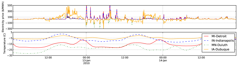
Figure 1: Real-time electricity prices and temperatures in four US cities over three days

With such energy-aware cloud management methods in mind, we propose a progressive SLA specification, where services are divided among multiple treatment categories, each under a different SLA with different availability and price values. Hence, different schedulers can be used for VM s in different treatment categories (or the same scheduler with different QoS constraint parameters). The goal of this approach is to allow different levels of energy-aware cloud management and thus achieve higher energy savings on VM s with lower availability requirements. What is given, therefore, are the schedulers for each treatment category, and the historical traces of generated schedules. What we have to find are the availability and price values that can be guaranteed in the SLAs for each treatment category and the optimal number of such SLAs to balance SLA flexibility and search difficulty for users.

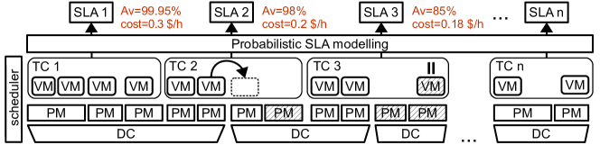
Figure 2: Progressive SLA specification

We illustrate this approach in Fig. 2. A cloud provider operates a number of VM s, each hosted on a physical machine (PM) located in one of the geographically-distributed data centers (DC). Each VM belongs to a treatment category (TC) that determines the type of scheduling that can be applied to it. For example, TC 1 is a high availability category where no actions are applied on running VM s. TC 2 is a category for moderate cloud management actions, such as live VM migrations (marked by an arrow) which result in short downtimes. TC 3 is a more aggressive category where VM s can be paused (marked as hatched with two vertical lines above it) for longer downtimes. Other TC s can be defined using other scheduling algorithms or by varying parameters, e.g. the maximum pause duration. The optimal number of TC s (and therefore also SLA s) $n$ is determined by analysing user SLA selection to have enough variety to satisfy most user types, yet not make the search too difficult, which we explore in Section 6. Aside from selecting the number of SLA s, another task is setting availability and price values for every SLA. As energy-aware cloud management that depends on geotemporal inputs introduces a degree of randomness into the resulting availability and price values of a VM, we can only estimate the values that can be guaranteed. We do this using a probabilistic SLA modelling method for analysing historical cloud management action traces to calculate the most likely worst-case availability and average energy cost for a VM in a TC. For the example in Fig. 2, sample values are given for the SLA s. SLA 1 might have an availability (Av) of $99.95\%$ and a high cost of $0.3$ $/h due to no energy-aware management, SLA 2 might have slightly lower values due to live migrations being applied on VM s in TC 2, SLA 3 might have even lower values due to longer downtimes caused by VM pausing… In the following section, we will show how to actually estimate availability and price values for the SLA s using probabilistic SLA modelling.

4 Probabilistic SLA Modelling

To estimate availability and price values that can be guaranteed in an SLA using probabilistic modelling for a certain TC, we require historical cloud management traces. Cloud management traces can be obtained through monitoring, but for evaluation purposes we simulate different scheduling algorithm behaviour.  VM price is estimated by accounting for the average energy costs. To calculate VM availability, we analyse the factors that cause VM downtime. While the downtime duration of the peak pauser scheduler can be specified beforehand, the total downtime caused by the migration scheduler depends on VM migration duration and rate as dictated by geotemporal inputs, so we individually analyse both factors.

4.1 Cloud Management Simulation

Our modelling method can be applied to different scheduling algorithms and cloud environments. To generate a concrete SLA offering for evaluation purposes, we consider a use case of a cloud consisting of six geographically distributed data centers. We use a dataset of electricity prices described in [4] and temperatures from the Forecast web service [1]. We represent a deployment with world-wide data center distribution shown in Fig. 3. Indianapolis and Detroit were used as US locations. Due to limited data availability, we modified data for Mankato and Duluth to resemble Asian locations and Alton and Madison to resemble European locations (using inter-continent differences in time zones and annual mean values). The effects of the migration and peak pauser scheduler are determined in a simulation using the Philharmonic cloud simulator we developed [7]. The cloud simulation parameters are summarised in Table 1. We illustrate the application of the presented methods with this use case as a running example.

Figure 3: Simulated world-wide data centers

duration	DCs	PMs	VMs
3 months	6	20	80

Table 1: Cloud simulation

4.2 Migration Duration

Even a live VM migration incurs a temporary downtime, in the stop-and-copy phase of VM memory transferring. A very accurate model, with less than 7% estimation errors, for calculating this downtime overhead is presented in [14]. The total VM downtime during a single live migration $T_{down}$ is a function of the VM’s memory $V_{mem}$, data transmission rate $R$, memory dirtying rate $D$, pre-copying termination threshold $V_{thd}$ and $T_{resume}$, the time necessary to resume a VM.

$$T_{down}=\frac{V_{mem}D^{n}}{R^{n+1}}+T_{resume}\quad\text{, where}\hskip 10.00002ptn=\bigg{\lceil}log_{\frac{D}{R}}\frac{V_{thd}}{V_{mem}}\bigg{\rceil}$$ (1)

All of the parameters can be determined beforehand by the cloud provider, except for $R$ and $D$ which depend on the dynamic network conditions and application-specific characteristics. Based on historical data, it is possible to reason about the range of these variables. In our running example, we assume a historical range from low to high values. $R$ values in the 10–1000 Mbit/s range were taken based on an independent benchmark of Amazon EC2 instance bandwidths. $D$ values from 1 kbit/s (to represent almost no memory dirtying) to 1 Gbit/s were taken (the maximum is not important, as will be shown). We assumed constant $V_{mem}=4GB,\ V_{thd}=1GB,\ T_{resume}=5s$, as these values do not affect the order of magnitude of $T_{down}$. We show how $T_{down}$ changes for different $R$ and $D$ in Fig. 4. Looking at the graph, we can see that higher $R$ and $D$ values result in convergence towards negligible downtime durations and the only area of concern is the peak happening when $R$ and $D$ are both very low. This happens, because close $R$ and $D$ values lead to a small number of pre-copying rounds and copying the whole VM under slow speeds leads to long downtimes. $T_{down}$ is under 400 s in the worst-case scenario,  which will be our SLA estimation as suggested in [5].

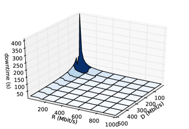
Figure 4: VM downtime during a live migration

4.3 Migration Rate

Aside from understanding migration effects, we need to analyse how often they occur, i.e. the migration rate. We present a method to analyse migration traces obtained from the cloud manager’s past operation. A histogram of migration rates for the migration traces from our running example described in Section 4.1 can be seen in Fig. 6. The two plots show different zoom levels, as there are few hours with higher migration rates. Most of the time, no migrations are scheduled, with one migration per hour happening about 3% of the time. 

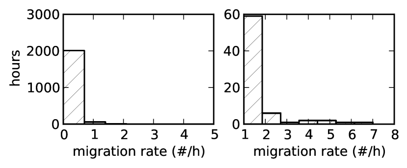
Figure 5: Hourly migration rate histogram

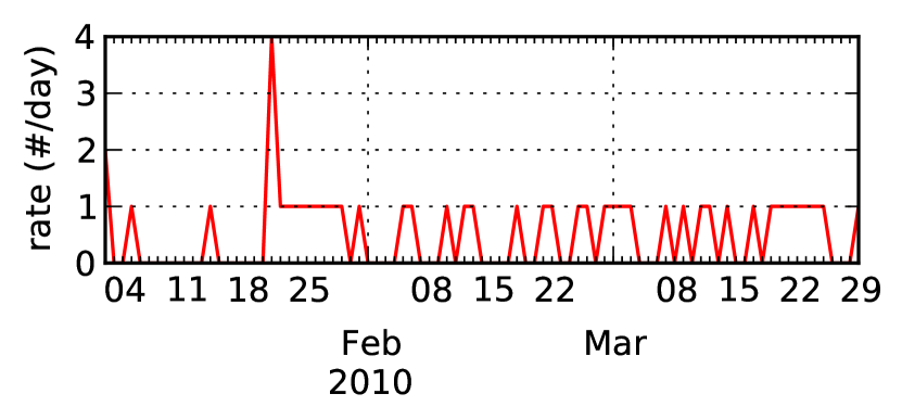
Figure 6: Aggregated worst-case migration rate

The idea is to group migrations per VM and process them in a function that aggregates migrations in intervals meaningful to the user. We consider an aggregation interval of 24 hours. The aggregated worst-case function counts the migrations per VM per day and selects the highest migration count among all the VM s in every interval. The output time series is shown in Fig. 6. There is one or zero migrations per VM most of the time, with an occasional case with a higher rate, such as the peak in January. Such peaks can occur due to more turbulent geotemporal input changes.

Given that this data is highly dependent of the scheduling algorithm used and the actual environmental parameters, fitting one specific statistical distribution to the data to get the desired percentile value would be hard to generalise for different use cases and might require manual modelling. Instead, we propose applying the distribution-independent bootstrap confidence interval method [8] to predict the maximum aggregated migration rate. For our migration dataset, the 95% confidence interval for the worst-case migration rate is from three to four migrations per day. 

4.4 SLA Options

By combining the migration rate and duration analyses, we can estimate the upper bound for the total VM downtime and, therefore, the availability that can be warranted in the SLA. We define availability ($Av$) of a VM as:

$$Av=1-\frac{\text{total VM downtime}}{\text{total VM lease time}}$$ (2)

For our migration dataset and the previously discussed migration duration and rate, we estimate the total downtime of a VM  controlled by the migration scheduler to be 27 minutes per day in the worst case, meaning we can guarantee an availability of 98.12%. We can precisely control the availability of the VM s managed by the peak pauser.

The average energy savings ($en\_savings$) for a VM running in a treatment category $TC_{i}$ can be calculated by comparing it to the high availability $TC_{1}$. From the already described simulation, we calculate $en\_cost$, the average cost of energy consumed by a VM  based on real-time electricity prices and temperatures. We divide the energy costs equally among VM s within a TC. This is an approximation, but serves as an estimation of the energy saving differences between TC s. We calculate energy savings as:

$$en\_savings(VM_{TC_{i}})=1-\frac{en\_cost(VM_{TC_{i}})}{en\_cost(VM_{TC_{1}})}$$ (3)

where $en\_cost(VM_{TC_{1}})$ is the average energy cost for a VM in $TC_{1}$ with no actions applied and $en\_cost(VM_{TC_{i}})$ is the average energy cost for a VM in the target $TC_{i}$.

The VM cost consists of several components.  Aside from $en\_cost$, $service\_cost$ groups other VM upkeep costs (manpower, hardware amortization, profit margin etc.) during a charge unit (typically one hour in infrastructure as a service (IaaS) clouds). We assume the service component to be charged linearly to the VM’s availability.

$$cost=en\_cost+Av\cdot service\_cost$$ (4)

To generate the complete SLA offering we consider an Amazon m3.xlarge instance which costs 0.280 $/h (Table 2) as a base VM with no energy-aware scheduling. Base instances with different resource values (e.g. RAM, number of cores) can be used, but this is orthogonal to the QoS requirements of availability that we consider and would not influence the energy-aware cloud management potential. Similarly, Amazon spot instances were not considered specially as they perform exactly the same as normal instances while running, as we explained in Section 2. We assumed the service component to be 0.1 $/h, about a third of the VM’s price. The prices of VM s controlled by the two energy-efficient schedulers were derived from it, applying $en\_savings$ obtained in the cloud simulation. The resulting SLA s are shown in Fig. 7. SLA 1 is the base VM. SLA 2 is the VM controlled by the migration scheduler. The remaining SLA s are VM s controlled by the peak pauser scheduler with downtimes uniformly distributed from 12.5% to 66.67% to represent a wide spectrum of options. We chose eight SLA s to analyse how SLA selection changes from the user perspective. We later show that this number is in the 95% confidence interval for being the optimal number of SLA s based on our simulation. We analyse a wider range of 1–60 offered SLA s and how they impact customer conversion from the cloud provider’s perspective in Section 6. The lines in the background illustrate value progression. $Av$ decreases only slightly for the migration SLA, yet the energy savings are significant due to dynamic VM consolidation and PM suspension. For peak pauser SLA s, availability and costs decrease linearly, from high to low values. The $en\_savings$ values are at first lower than those attainable with the migration scheduler, as the peak pauser scheduler cannot migrate VM s to a fewer number of PM s, but can only pause them for a certain time. With lower availability requirements, however, the peak pauser can achieve higher $en\_savings$ and lower prices, which could not be reached by VM migrations alone.

Figure 7: SLA s generated for different TC s

type	m3.xlarge
Av	99.95%
cost	0.28 $/h
service	0.1 $/h

Table 2: Base VM

5 User Modelling

Knowing the SLA offering, the next step is to model user SLA selection in order to analyse the benefits of our progressive SLA specification. We first describe how we derive user requirements and then the utility model used to simulate user SLA selection based on their requirements.

5.1 User Requirements Model

To model user requirements, we use real traces of web and high-performance computing (HPC) workload, since I/O-bound web and CPU-bound HPC applications represent two major usage patterns of cloud computing. As we do not have data on availability requirements of website owners, we generate this dataset based on the frequency of end user HTTP requests directed at different websites and counting missed requests, similarly to how reliability is determined from the mean time between failures [17]. A public dataset of HTTP requests made to Wikipedia [19] is used. To obtain data for different websites, we consider Wikipedia in each language as an individual website, because of its unique group of end users (different in number and usage pattern). In this scenario we consider a website owner to be the user of an IaaS service (not to be confused with the end user, a website visitor). The number of HTTP requests for a small subset of four websites (German, French, Italian and Croatian Wikipedia denoted by their two-letter country codes) is visualised in Fig. 8 (a) for illustration purposes (we use the whole dataset with 38 websites for actual requirements modelling). The data exemplifies significant differences in amplitudes. Users of the German Wikipedia send between 1k and 2k requests per minute, while the Italian and Croatian Wikipedia have less than 300 requests per minute. Due to this variability, we assume that different Wikipedia websites represent diverse requirements of website owners. We model availability requirements by applying a heuristic – a website’s required availability is the minimum necessary to keep the number of missed requests below a constant threshold (we assume 100 requests per hour). Using this heuristic, we built an availability requirements dataset for the web user type from 5.6 million requests divided among 38 Wikipedia language subdomains. The resulting availability requirement histogram can be seen in Fig. 8 (b). It follows an exponential distribution (marked in red). There is a high concentration of sites that need almost full availability, with a long tail of sites that need less (0.85–1.0).

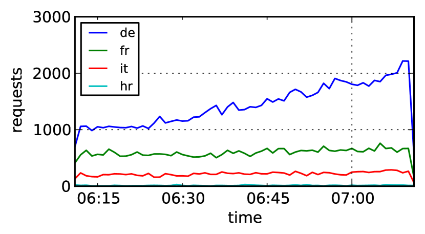
(a) Wikipedia requests per minute

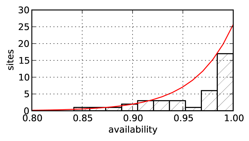
(b) Wikipedia availability distribution

Figure 8: Web user modelling

For HPC workload, we use a dataset of job submissions made to Grid’5000 (G5k) [2], a distributed job submission platform spread across 9 locations in France. The number of jobs submitted by a small subset of users is visualised in Fig. 9 (a). While some users submit jobs over a wide period (blue), others only submit jobs in small bursts (green), but the load is not nearly as constant as the web requests from the Wikipedia trace. To model HPC users’ availability requirements, where jobs have variable duration as well as rate (unlike web requests, which typically have a very short duration), we use another heuristic. Every user’s availability requirement is mapped between a constant minimum availability (we assume 0.5) and full availability using $mean\_duration\cdot mean\_rate$, which stands for mean job duration and mean job submission rate per user. Using this heuristic, we built a dataset of availability requirements for the HPC user type from jobs submitted over 2.5 years by 481 G5k users. The resulting availability requirement distribution (normalised such that the area is 1) can be seen in Fig. 9 (b). The distribution marked red again follows an exponential distribution (the first bin, cut off due to the zoom level, shows a density of 100), but with the tail facing the opposite direction than the web requirements. HPC users submit smaller and less frequent jobs most of the time, with a long tail of longer and/or more frequent jobs (from 0.5 to 0.75).

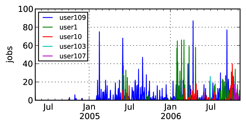
(a) G5k example job submissions

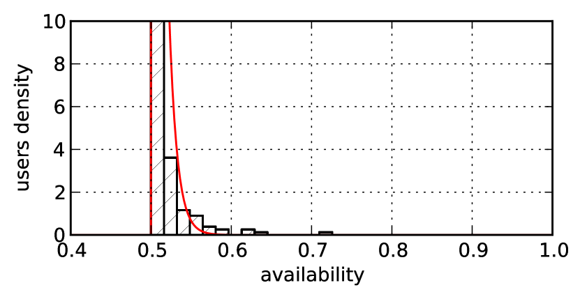
(b) G5k availability distribution

Figure 9: HPC user modelling

Every user’s willingness to pay (WTP) is derived by multiplying his/her availability requirement with the base VM price and adding Gaussian noise $\mathcal{N}(0,\,0.05^{2})$ to express subjective value perception. We selected the noise standard deviation to get positive WTP values considering the availability model. The resulting WTP histogram is shown in Fig. 11. It can be seen that HPC users have lower WTP values, but there is also an overlap area with web users who have similar requirements.

5.2 Utility Model

The utility-based model is used to simulate how users select services based on their requirements. We use a quasi-linear utility function adopted from multi-attribute auction theory [10] to quantify the user’s preference for a provided SLA. The utility is calculated by multiplying the user’s SLA satisfaction score with WTP and subtracting the VM cost charged by the provider. The utility for user $i$ from selecting a VM instance type $t$ with availability $Av_{t}$ is calculated as:

$$U_{i}(VM_{t})=WTP_{i}\cdot f_{i}(Av_{t})-cost(VM_{t})$$ (5)

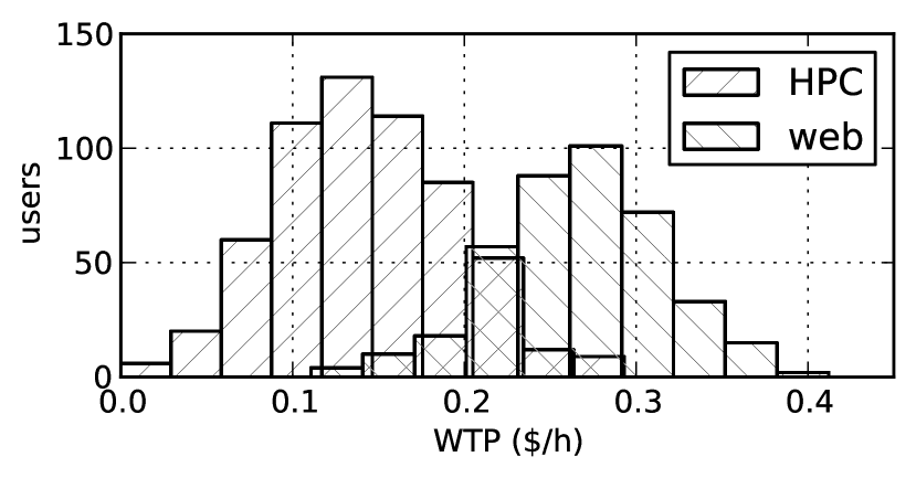
Figure 10: WTP histogram

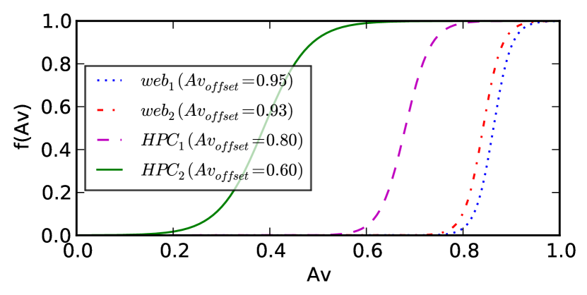
Figure 11: SLA satisfaction function

where $f_{i}(Av_{t})$ is the user’s satisfaction with the offered VM’s availability. We model it using a mapping function $f_{i}:[0,1]\to[0,1]$, extended from [10] with variable slopes:

$$f_{i}(Av_{t})=\frac{\gamma}{\gamma+\beta e^{Av_{offset_{i}}^{2}\alpha(Av_{offset_{i}}-Av_{t})}}$$ (6)

where $Av_{offset_{i}}$ is the required availability specific to each user, which we select based on the exponential models of Wikipedia and G5k data presented earlier. $\alpha$, $\beta$ and $\gamma$ are positive constants common for all users, which we set to 60, 0.01 and 0.99 respectively. These values were chosen for a satisfaction of close to 1 for the desired availability value and a steep descent towards 0 for lower values, similar to earlier applications of this satisfaction function [10]. The slope of the function also depends on $Av_{offset_{i}}$, to model that users who require a lower availability have a wider range of acceptable values. The mapping function is visualised in Fig. 11 for a small sample of two HPC and two web users. We can see that for the two web users, the slope is almost the same and very steep (at 0.93 their satisfaction is close to 1 and at 0.8 it is almost 0). The $HPC_{1}$ user is similar to the web users, only with lower availability requirements and a slightly wider slope. The $HPC_{2}$ user has low requirements and a wide slope from an availability of 0.2 to 0.6. Later in our evaluation, we generate 1000 users, each with different mapping functions, distributed according to the user requirements model.

User $i$ chooses a VM instance type $VM_{selected}$ offering the best utility value:

$$U_{i}(VM_{selected})=\max_{\forall t}\ U_{i}(VM_{t})$$ (7)

unless all types result in a negative utility, in which case the user selects none. Additionally, we model search difficulty by defining $P_{stop}$, a probability that a user will give up the search after an SLA has been examined. We model this probability as increasing after every new SLA check, by having $P_{stop_{j}}=j\cdot check\_cost$, where $j$ is the number of checks already performed and $check\_cost$ is a constant parameter standing for the probability of stopping after the first check. Based on every user’s requirements and the SLA offering, $min\_checks$ is the minimum number of checks necessary to reach a VM type that yields a positive $U_{i}(VM)$. We define $P_{quit}$ to be the total probability that a user will quit the search before reaching a positive-utility SLA. By applying the chain probability rule, we can calculate $P_{quit}$ as:

$$P_{quit}={\sum}_{j=1}^{min\_checks-1}P_{stop_{j}}\prod_{k=1}^{j-1}(1-P_{stop_{k}})$$ (8)

The outer sum is the joint distribution of all possible stop events that may occur for a user and the inner product stands for all event outcomes when searching continued until the $j$-th event was realised as stopping. We use this expression in the evaluation as a measure of difficulty for users to find a matching SLA.

6 Evaluation

In this section we describe the simulation of the proposed progressive SLA specification using user models based on real data traces and analyse the results.

6.1 Simulation Environment

The simulation parameters are summarised in Table 3. The first step of the simulation is to generate a population of web and HPC users based on the requirement models derived from the Wikipedia and Grid’5000 datasets, respectively. We simulated 1000 users to represent a population with enough variety to explore different WTP and availability requirements. We assume the ratio between web and HPC users of 1 : 1.5, based on an anlysis of a real system performed in [15]. We determine each user’s WTP from the desired availability with Gaussian noise, as already explained in the previous section. The SLA offering was derived from the migration and peak pauser scheduler using the probabilistic modelling technique (Section 4). For the examination of SLA selection from the user’s perspective, the eight SLA s we already defined in Section 4.4 were used. To examine the cloud provider’s perspective, we evaluated 1–60 SLA s, doing 100 simulation runs per offering to calculate the most likely optimal number of SLA s. A $check\_cost$ of 0.015 is selected to initially start with a low chance of the user quitting and then subsequently increase it for every SLA check per Eq. 8. The same $\alpha,\ \beta,\ \gamma$ values that we already explained in the previous section were set that result in a utility of 1 for the required availability and a gradual decline towards a utility of 0 for lower availabilities. The core of the simulation is to determine each user’s SLA selection (if any) based on the utility model (Section 5).

Table 3: Simulation settings

Parameter	users	web : HPC	#SLAs	runs	$check\_cost$	$\alpha$	$\beta$	$\gamma$
Value	1000	1 : 1.5	1–60	100	0.015	60	0.01	0.99

6.2 User Benefits

Simulation results showing the distribution of users among the eight offered SLA s from Section 4.4 are presented in Fig. 13. Different colours are used for web and HPC users types. It can be seen that most of the users successfully found a service that matches their requirements, with less than 5% of unmatched requests. The majority of HPC users are distributed between SLA 7 and 8 offering 42% and 33% availability, respectively. The majority of web users selected SLA 2, the migration scheduler TC, due to its high availability comparable to a full availability service, but a more affordable price due to the energy cost savings. 26% of web users opted for SLA 3, the peak pauser instance which still offers a high availability (87.5%), but at almost half the price of SLA 2.

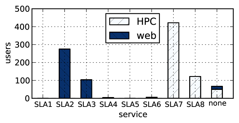
Figure 12: Simulated service selection

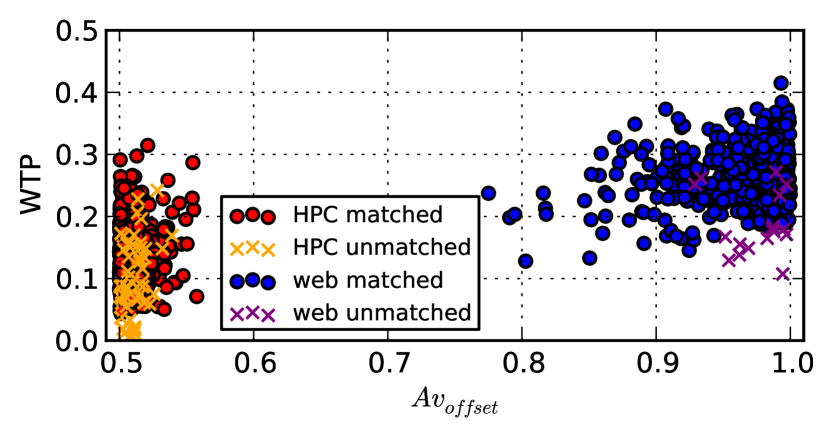
Figure 13: Matched and unmatched users

The distribution of unmatched users who did not select any of the offered services (where utility was negative for all SLA s) is shown alongside the matched users in Fig. 13, showing their $Av_{offset}$ and WTP values. We can see that unmatched users have low WTP values, the cause of them not being able to find a suitable service option.

6.3 Cloud Provider Benefits

Customer conversion means the number of users who looked at the SLA offering and found an SLA that matches their needs. This metric is an indicator of the provider’s economic success.  To compare the multiple treatment category system with the traditional way of only having a full availability option, we simulated different SLA offerings.  Fig. 15 shows customer conversion with colour indicating the selection distribution for different offering combinations of the eight previously examined SLA s. Customer conversion growth can be seen with more service types, due to users having a higher chance of finding a category that matches their requirements.  With SLA s 1–2 offered, only SLA 2 was selected, as it still offers a high-enough availability to satisfy user requirements and the price is lower than in SLA 1. As we widen the offering, more SLA s get selected, but the majority of users choose among two SLA s that best suit the two user types that we modelled. Still, a small number of users select other SLA s (SLA 3 and, if offered, SLA 8) which better suit their needs. SLA 5 is never selected due to user requirements and in real clouds such SLA s should be removed to simplify selection.

The introduced service types can be managed in a more energy efficient manner. The average energy savings weighted based on the lease time per VM for the SLA 1-8 offering, compared to the current 99.95% availability Amazon instances represented by SLA 1, are $39\%$. Full annual lease time was assumed for web users (as web applications are typically running all the time) and was varied based on job runtime and frequency for HPC users (we assume that a VM is provisioned just to perform the submitted job). This shows that more energy efficient management is possible if users declare the QoS levels they require through SLA selection. For the SLA 1-8 scenario, where $5.89\times$ more users can be converted and the annual lease times explained above, a $43\%$ revenue increase is calculated from the service component of the selected VM s. Exact numbers depend on the user type ratio that will vary between cloud providers. 

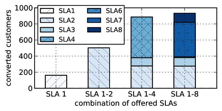
Figure 14: Matched users per SLA combination

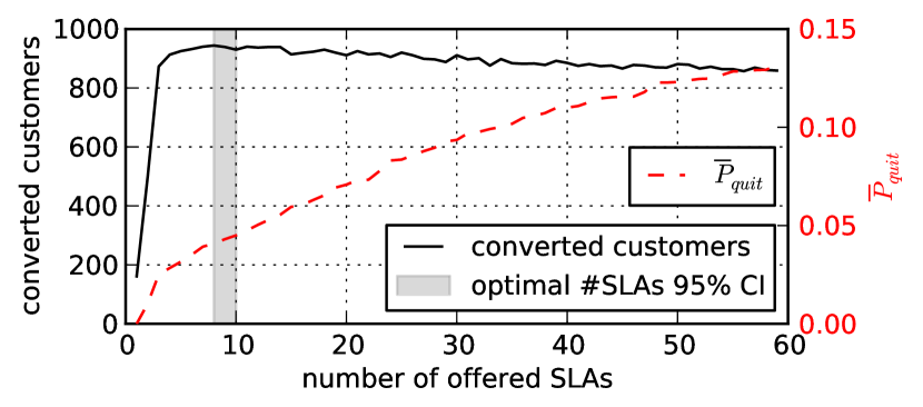
Figure 15: Users and $\overline{P}_{quit}$ per SLA number

To find the optimal number of offered SLA s, we performed a simulation where we explore customer conversion for a higher number of SLA s. The extra SLA s were generated for the peak pauser scheduler, which allows for arbitrary control of VM availability and price. The peak pauser SLA s were uniformly interpolated between full and no availability to avoid duplicates. Fig. 15 shows how the number of offered SLA s affects the user conversion count and $\overline{P}_{quit}$, the mean $P_{quit}$ value over all the users (including unmatched ones). After an initial linear growth, we can see that the number of users begins to stagnate and slowly decrease. Once a sufficient offering to satisfy the majority of users is achieved, adding extra SLA options only increases search difficulty. This is seen from the steadily increasing $\overline{P}_{quit}$, the probability that a user will quit the search before finding a positive-utility SLA. For our scenario, the optimal number of converted customers is achieved between 6 and 14 SLA s, depending on the $P_{quit}$ random variable realisations. By applying the bootstrap confidence interval method, we calculate the 95% confidence interval (CI) for the optimal number of SLA s to be between 8 and 10.

7 Conclusion

We presented a novel progressive SLA specification suitable for energy-aware cloud management. We obtained cloud management traces from two schedulers optimised for real-time electricity prices and temperature-dependent cooling efficiency. The SLA s are derived using a method for a posteriori probabilistic modelling of cloud management data to estimate upper bounds for VM availability, energy savings and the resulting VM prices. The SLA specification is evaluated in a utility-based user SLA selection simulation using realistic workload traces from Wikipedia and Grid’5000. Results show mean energy savings per VM of up to $39\%$ due to applying more aggressive energy preservation actions on users with lower QoS requirements. Furthermore, a wider spectrum of user types with requirements not matched by the traditional high availability VM s can be reached, increasing customer conversion.

In the future, we plan on expanding the probabilistic model with time series forecasting for more accurate SLA metrics. Additional TC s could be added to represent other cloud management methods, such as the kill-and-restart pattern used on stateless application containers in modern web application architectures. We also plan to explore SLA violation detection and how it could be integrated into our SLA specification. Furthermore, as predictions change based on day-night and seasonal changes, exploring time-changing SLA s in the manner of stocks and bonds to match the volatile geotemporal inputs would be feasible.

Acknowledgements. The work described in this paper has been funded through the Haley project (Holistic Energy Efficient Hybrid Clouds) as part of the TU Vienna Distinguished Young Scientist Award 2011.

References

- [1] Forecast, http://forecast.io/
- [2] GWA-t-2 grid5000, http://gwa.ewi.tudelft.nl/datasets/gwa-t-2-grid5000
- [3] Abbasi, Z., Mukherjee, T., Varsamopoulos, G., Gupta, S.K.S.: Dynamic hosting management of web based applications over clouds. In: 2011 18th International Conference on High Performance Computing (HiPC). pp. 1–10 (Dec 2011)
- [4] Alfeld, S., Barford, C., Barford, P.: Toward an analytic framework for the electrical power grid. In: Proceedings of the 3rd International Conference on Future Energy Systems: Where Energy, Computing and Communication Meet. pp. 9:1–9:4. e-Energy ’12, ACM, New York, NY, USA (2012)
- [5] Berndt, P., Maier, A.: Towards sustainable IaaS pricing. In: Altmann, J., Vanmechelen, K., Rana, O.F. (eds.) Economics of Grids, Clouds, Systems, and Services, pp. 173–184. No. 8193 in Lecture Notes in Computer Science, Springer International Publishing (Jan 2013)
- [6] Chen, J., Wang, C., Zhou, B.B., Sun, L., Lee, Y.C., Zomaya, A.Y.: Tradeoffs between profit and customer satisfaction for service provisioning in the cloud. In: Proceedings of the 20th International Symposium on High Performance Distributed Computing. pp. 229–238. HPDC ’11, ACM, New York, NY, USA (2011)
- [7] Dražen Lučanin: Philharmonic (2014), https://philharmonic.github.io/
- [8] Efron, B., Tibshirani, R.J.: An Introduction to the Bootstrap. CRC Press (May 1994)
- [9] Ibrahim, S., He, B., Jin, H.: Towards pay-as-you-consume cloud computing. In: 2011 IEEE International Conference on Services Computing (SCC). pp. 370–377 (Jul 2011)
- [10] Jrad, F., Tao, J., Knapper, R., Flath, C.M., Streit, A.: A utility-based approach for customised cloud service selection. Int. J. Computational Science and Engineering (forthcoming)
- [11] Koomey, J.G.: Worldwide electricity used in data centers. Environmental Research Letters 3, 034008 (Jul 2008)
- [12] Le, K., Bianchini, R., Zhang, J., Jaluria, Y., Meng, J., Nguyen, T.D.: Reducing electricity cost through virtual machine placement in high performance computing clouds. In: Proceedings of 2011 International Conference for High Performance Computing, Networking, Storage and Analysis. pp. 22:1–22:12. SC ’11, ACM, New York, NY, USA (2011)
- [13] Lin, M., Liu, Z., Wierman, A., Andrew, L.: Online algorithms for geographical load balancing. In: Green Computing Conference (IGCC), 2012 International. pp. 1–10 (Jun 2012)
- [14] Liu, H., Xu, C.Z., Jin, H., Gong, J., Liao, X.: Performance and energy modeling for live migration of virtual machines. In: Proceedings of the 20th international symposium on High performance distributed computing. pp. 171–182 (2011)
- [15] Liu, Z., Chen, Y., Bash, C., Wierman, A., Gmach, D., Wang, Z., Marwah, M., Hyser, C.: Renewable and cooling aware workload management for sustainable data centers. In: Proceedings of the 12th ACM SIGMETRICS/PERFORMANCE joint international conference on Measurement and Modeling of Computer Systems. pp. 175–186. SIGMETRICS ’12, ACM, New York, NY, USA (2012)
- [16] Lučanin, D., Brandic, I.: Take a break: cloud scheduling optimized for real-time electricity pricing. In: Cloud and Green Computing (CGC), 2013 Third International Conference on. pp. 113–120. IEEE (2013)
- [17] O’Connor, P., Kleyner, A.: Practical reliability engineering. John Wiley & Sons (2011)
- [18] Qureshi, A., Weber, R., Balakrishnan, H., Guttag, J., Maggs, B.: Cutting the electric bill for internet-scale systems. SIGCOMM Comput. Commun. Rev. 39(4), 123–134 (Aug 2009)
- [19] Urdaneta, G., Pierre, G., van Steen, M.: Wikipedia workload analysis for decentralized hosting. Elsevier Computer Networks 53(11), 1830–1845 (Jul 2009)
- [20] Vieira, C.C.A., Bittencourt, L.F., Madeira, E.R.M.: Towards a PaaS architecture for resource allocation in IaaS providers considering different charging models. In: Altmann, J., Vanmechelen, K., Rana, O.F. (eds.) Economics of Grids, Clouds, Systems, and Services, pp. 185–196. No. 8193 in Lecture Notes in Computer Science, Springer International Publishing (Jan 2013)
- [21] Weron, R.: Modeling and Forecasting Electricity Loads and Prices: A Statistical Approach. Wiley, 1 edn. (Dec 2006)
- [22] Xu, H., Feng, C., Li, B.: Temperature aware workload management in geo-distributed datacenters. In: Presented as part of the 10th International Conference on Autonomic Computing. pp. 303–314. USENIX, Berkeley, CA (2013)
- [23] Zhou, R., Wang, Z., McReynolds, A., Bash, C.E., Christian, T.W., Shih, R.: Optimization and control of cooling microgrids for data centers. In: Thermal and Thermomechanical Phenomena in Electronic Systems (ITherm), 2012 13th IEEE Intersociety Conference on. pp. 338–343. IEEE (2012)