Charge-exchange excitations with finite range interactions including tensor terms

Abstract

We study charge-exchange excitations in doubly magic-nuclei by using a self-consistent Hartree-Fock plus Random Phase Approximation model. We use four Gogny-like finite-range interactions, two of them containing tensor forces. We investigate the effects of the various parts of the tensor forces in the two computational steps of our model, and we find that their presence is not negligible and improves the agreement with the experimental data.

I Introduction

The study of charge-exchange excitations in neutron-rich nuclei is an important issue not only for its intrinsic interest ost92 ; ich06 ; fuj11 , but also for the special role that these excitations play in many astrophysical processes such as beta decay, electron capture and r-process in nucleosynthesis arn07 . From the theoretical point of view, it is desirable to have models which can describe these excitations in every nucleus, also in systems too short-lived to allow for experimental studies.

Collective nuclear excitations have been successfully described by the Random Phase Approximation (RPA) theory spe91 whose extension to handle charge-exchange excitations was formulated some time ago hal67 ; lan80 ; aue81 ; aue83 . The description of available data has been conducted by using a phenomenological input of the RPA, where the single particle (s.p.) wave functions and energies were generated by mean-field potentials, for example of Woods-Saxon type, and the effective nucleon-nucleon interaction had Landau-Migdal form spe91 . From these studies it has been possible to select the value of the parameter defining the spin-isospin dependent term of the interaction ost92 ; ich06 . The application of this phenomenological approach is limited to nuclei whose ground state properties are experimentally known. The theoretical exploration of nuclei in the experimentally unknown regions of the nuclear chart requires a more microscopic approach.

In this perspective, the combination of Hartree-Fock (HF) and RPA calculations carried out with a unique effective interaction has been able to provide a good description of known nuclear properties in a wide range of the nuclear chart, from light nuclei, around the oxygen region, up to very heavy nuclei such as the uranium. This success induces to believe that this computational scheme can provide good predictions of the properties of exotic nuclei which will be produced in the next few years in radioactive ion beams facilities. This possibility has increased the interest in defining more precisely the details of the self-consistent HF+RPA calculations.

Self-consistent studies of charge-exchange excitations have been conducted mainly with zero-range Skyrme-type interactions ham00 ; fra07 . Recently, these interactions have been implemented with tensor terms, and the effects of these new terms on charge-exchange excitations have been studied bai09a ; bai09b ; bai10 ; bai11a ; bai11b ; min13 . Other authors have studied charge-exchange excitations within quasi-particle RPA using the Bonn-A two-body potential in Woods-Saxon s.p. bases. bes12 ; civ14 .

In this work we apply a HF+RPA computational scheme based on Gogny-like finite-range interactions to study isobaric analog states, Gamow-Teller, spin-quadrupole and spin-dipole excitations in ⁴⁸Ca, ⁹⁰Zr  and ²⁰⁸Pb. Our first task is to test the validity of our model against the available experimental data. We use four parametrizations of the Gogny-like interaction. The D1S ber91 and D1M gor09 forces contain the traditional set of parameters of the original Gogny interaction. Following the procedure outlined in Ref. gra13 we add to these two parametrizations a tensor force, and we call D1ST2c and D1MT2c these new interactions. The second task of the present work is the study of the tensor effects on the various observables related to charge-exchange excitations.

The paper is structured as follows. In Sec. II we briefly present our HF+RPA model, and also the quantities we calculate to compare our results with the experiment. The interactions we use in this investigation are discussed in Sect. III. In the same section we provide some information about the numerical details of the calculations. We dedicate Sect. IV to the presentation of our results. In the first part of the section we compare those results obtained by using interactions with and without tensor forces. In the second part we study the effects of the various terms of the interaction on the different charge-exchange excitations we have considered. Finally, in Sect. V we summarize the main results of our investigation and we draw our conclusions.

II Model

The RPA theory describes the excited state of a many-body system as a linear combination of particle-hole and hole-particle excitations. Because the states of the nucleus are characterized by a total angular momentum $J$, it is convenient to work in an angular momentum coupling scheme, where the RPA excited states are eigenstates of the $\boldsymbol{J}^{2}$ and $J_{z}$ operators:

$$|JM\rangle\,=\,\sum_{qk}\left[X_{qk}^{J}\,{\cal A}^{{\dagger}}_{qk}(JM)\,-\,Y_{qk}^{J}\,\tilde{\cal A}_{qk}(J{M})\,\right]|0\rangle\,,$$ (1)

where $X^{J}$ and $Y^{J}$ are the RPA amplitudes and we have defined

$${\cal A}^{{\dagger}}_{qk}(JM) = \sum_{\mu_{q}\mu_{k}}\,\langle j_{q}\mu_{q}j_{k}\mu_{k}|JM\rangle\,a^{{\dagger}}_{j_{q},\mu_{q}}\,(-1)^{j_{k}+\mu_{k}}\,a_{j_{k},-\mu_{k}}\,,$$ (2)

$$\tilde{\cal A}_{qk}(J{M}) = \sum_{\mu_{q}\mu_{k}}\,(-1)^{J-M}\,\langle j_{q}\mu_{q}j_{k}\mu_{k}|J-M\rangle\,a^{{\dagger}}_{j_{k},\mu_{k}}\,(-1)^{j_{q}+\mu_{q}}\,a_{j_{q},-\mu_{q}}\,.$$ (3)

In the above equations $a^{{\dagger}}$ and $a$ indicate the usual creation and annihilation single nucleon operators, $k$ the quantum numbers characterizing a s.p. state below the Fermi surface and $q$ those of a state above it. Besides, $j$ and $\mu$ are, respectively, the angular momentum and its projection on the $z$-axis of the nucleon. In the above expressions, we understood the explicit dependence of the excited state and of the $X$ and $Y$ amplitudes on the parity $\Pi$ and on the excitation energy $\omega$.

Charge-exchange excitations can be classified as isospin lowering T_-  when the hole is a neutron and the particle is a proton, and isospin rising T₊  when the hole is a proton and the particle is a neutron. We use the usual convention of $p$ and $n$ for a proton and a neutron state, respectively, and the bar to indicate a hole state, therefore we have $p\overline{n}$ pairs in T_-  , and $n\overline{p}$ pairs in T₊  excitations.

Charge conservation allows to write the secular RPA equations in a compact form lan80 ; aue81 . We define two new variables $U^{J}$ and $W^{J}$ such as in the T_-  channel we have

$$X^{J}_{p\overline{n}}\,=\,U^{J}_{p\overline{n}}\,,\,\,\,Y^{J}_{n\overline{p}}\,=\,W^{J}_{n\overline{p}}\,\,\,{\rm and}\,\,\,\omega\,=\,\Omega\,,$$ (4)

and in the T₊  channel

$$X^{J}_{n\overline{p}}\,=\,W^{J}_{n\overline{p}}\,,\,\,\,Y^{J}_{p\overline{n}}\,=\,U^{J}_{p\overline{n}}\,\,\,{\rm and}\,\,\,\omega\,=\,-\Omega\,.$$ (5)

where we have indicated with $\omega$ the RPA excitation energy. The normalization of the RPA excited states (1) implies

$$\sum_{p\overline{n}}\,(U^{J}_{p\overline{n}})^{2}\,-\,\sum_{n\overline{p}}\,(W^{J}_{n\overline{p}})^{2}\,=\,\pm 1\,,$$ (6)

where the plus sign is for the T_-  excitations and the minus sign for T₊  ones.

With these definitions we write the RPA secular equations as

$$\begin{bmatrix}A^{J}_{p\overline{n}p^{\prime}\overline{n}^{\prime}}&B^{J}_{p\overline{n}n^{\prime}\overline{p}^{\prime}}\\ -B^{J}_{n\overline{p}p^{\prime}\overline{n}^{\prime}}&-A^{J}_{n\overline{p}n^{\prime}\overline{p}^{\prime}}\\ \end{bmatrix}\begin{bmatrix}U^{J}_{p^{\prime}\overline{n}^{\prime}}\\ W^{J}_{n^{\prime}\overline{p}^{\prime}}\\ \end{bmatrix}=\Omega\begin{bmatrix}U^{J}_{p\overline{n}}\\ W^{J}_{n\overline{p}}\\ \end{bmatrix}\,.$$ (7)

where $A$ and $B$ are expressed in terms of the interaction matrix elements and s.p. energies as:

$$A^{J}_{abcd} = (\epsilon_{a}-\epsilon_{b})\,\delta_{bc}\,\delta_{ad}\,+\,\overline{V}^{J}_{abcd}\,,$$ (8)

$$B^{J}_{abcd} = (-1)^{j_{c}-j_{d}-J}\,\overline{V}^{J}_{abdc}\,.$$ (9)

In the above equations, we have indicated with $\epsilon$ the s.p. energies, and with the symbol $\overline{V}^{J}_{abcd}$ the antisymmetrized matrix element of the interaction:

$$\overline{V}^{J}_{abcd} = \sum_{K}\,(-1)^{j_{b}+j_{c}+K}\,\sqrt{2K+1}\left\{\begin{array}[]{ccc}j_{a}&j_{b}&J\\ j_{c}&j_{d}&K\\ \end{array}\right\}$$ (13)

$$\hskip 19.91684pt\left[\langle j_{a}j_{d}K\|V\|j_{b}j_{c}K\,\rangle\,-\,(-1)^{j_{b}+j_{c}+K}\,\langle j_{a}j_{d}K\|V\|j_{c}j_{b}K\rangle\right]\,.$$

In the above equation, the double bar symbol $\|$ indicates the reduced matrix element of the angular part.

The diagonalization of the system (7) produces at the same time the solutions for T_-  and T₊  excitations. For a given excitation multipole, the charge-exchange RPA solution provides the set of excitation energies, and, for each excited state, the full set of RPA amplitudes $X^{J}$ and $Y^{J}$.

The strength function of the transition between the ground state and an excited state $|J^{\pi};\omega\rangle$ of a nucleus with $A$ nucleons induced by a one-body transition operator of the type

$${\cal Q}_{J^{\pi},M}^{\alpha\pm}\,=\,\sum_{i=1}^{A}\,{\eta}_{J^{\pi},M}^{\alpha\pm}(i)\,,$$ (14)

can be expressed as

$$\Gamma_{J^{\pi}}^{\alpha\pm}(\omega) = \sum_{M}|\langle J^{\pi},M;\omega|{\cal Q}_{J^{\pi},M}^{\alpha\pm}|0\rangle|^{2}$$ (15)

$$= \left|\sum_{qk}\left(X^{J}_{qk}\,\langle q\|{\eta}_{J^{\pi}}^{\alpha\pm}\|k\rangle\,+\,(-1)^{j_{q}-j_{k}+J+1}\,Y^{J}_{qk}\,\langle k\|{\eta}_{J^{\pi}}^{\alpha\pm}\|q\rangle\right)\right|^{2}\,,$$

where $M$ is the $z$ axis projection of $J$. In the second line of Eq. (15), we have applied the Wigner-Eckart theorem edm57 , therefore we dropped the explicit dependence on $M$. Also in this case, as in Eq.(1), we understand the dependence of the $X$ and $Y$ amplitudes on the parity $\Pi$ and of the excitation energy $\omega$ of the excitation. Since we consider even-even nuclei only, the angular momentum and the parity, $J^{\pi}$, of the excitation coincide with those of the nuclear final state. We list here below the transition operators which we consider in this work. For the excitation of the $0^{+}$ states, the isobaric analog states, we consider the Fermi (F) operator

$${\cal Q}_{0^{+},0}^{{\rm F}\pm}\,=\,\sum_{i=1}^{A}\,t_{\pm}(i)\,.$$ (16)

For the excitation of the $1^{+}$ states we use the Gamow-Teller (GT) operator

$${\cal Q}_{1^{+},M}^{{\rm GT}\pm}\,=\,\sum_{i=1}^{A}\,\mbox{\boldmath$\sigma$}_{M}(i)\,t_{\pm}(i)\,=\,\sqrt{4\pi}\,\sum_{i=1}^{A}\,[Y_{0}(i)\otimes\mbox{\boldmath$\sigma$}(i)]^{1}_{M}\,t_{\pm}(i)\,,$$ (17)

and the spin quadrupole (SQ) operator

$${\cal Q}_{1^{+},M}^{{\rm SQ}\pm}\,=\,\sum_{i=1}^{A}\,r^{2}_{i}\,[Y_{2}(i)\otimes\mbox{\boldmath$\sigma$}(i)]^{1}_{M}\,t_{\pm}(i)\,.$$ (18)

Finally, we consider the excitations induced by the spin dipole (SD) operator

$${\cal Q}_{J^{-},M}^{{\rm SD}\pm}\,=\,\sum_{i=1}^{A}\,r_{i}\,[Y_{1}(i)\otimes\mbox{\boldmath$\sigma$}(i)]^{J}_{M}\,t_{\pm}(i)\,,$$ (19)

which excites the multipoles $0^{-}$, $1^{-}$ and $2^{-}$. In this case, apart from the strength functions corresponding to each individual multipolarity, also the total strength

$$\Gamma^{{\rm SD}\pm}(\omega)\,=\,\sum_{J^{\pi}=0^{-},1^{-},2^{-}}\Gamma_{J^{\pi}}^{{\rm SD}\pm}(\omega)$$ (20)

has been calculated. In the previous equations we used $t_{\pm}=\tau_{\pm}/2$ where $\tau_{+}$ and $\tau_{-}$ are the isospin operators transforming, in our convention, a proton into a neutron and vice-versa, respectively. Furthermore, we have indicated with $Y_{L}$ the spherical harmonics and with $\sigma$ the Pauli matrix operator acting on the spin variable. The symbol $[A\otimes B]$ indicates the usual tensor product between irreducible sperical tensors edm57 . The expressions of the reduced matrix elements of Eq. (15) are given in Appendix A for the operators we have presented above.

The sum rules are an important tool to investigate the global properties of the charge-exchange excitations. In order to obtain the sum rule expressions, it is useful to define the energy moments:

$$m_{\lambda}^{\alpha\pm}\,=\,\sum_{J^{\pi}}\,m_{\lambda}({\cal Q}^{\alpha\pm}_{J^{\pi}})\,,$$ (21)

where

$$m_{\lambda}({\cal Q}^{\alpha\pm}_{J^{\pi}})\,=\,\int_{0}^{\infty}{\rm d}\omega\,\omega^{\lambda}\,\Gamma_{J^{\pi}}^{\alpha\pm}(\omega)\,.$$ (22)

According to these expressions, we define the centroid energy of an excitation induced by the $\alpha$-type operator as

$${\omega}_{\rm cen}^{\alpha\pm}\,=\,\frac{m_{1}^{\alpha\pm}}{m_{0}^{\alpha\pm}}\,.$$ (23)

In the case of the SD transitions, we have also calculated the centroid of the distributions of the individual multipolarities

$${\omega}_{{\rm cen},J^{\pi}}^{{\rm SD}\pm}\,=\,\frac{m_{1}({\cal Q}^{{\rm SD}\pm}_{J^{\pi}})}{m_{0}({\cal Q}^{{\rm SD}\pm}_{J^{\pi}})}\,.$$ (24)

By using the property $(\tau_{\pm})^{{\dagger}}=\tau_{\mp}$, and the completeness of the RPA excited states we have that aue81 ; aue83

$$m_{0}^{\alpha-}\,-\,m_{0}^{\alpha+} = \sum_{J^{\pi}}\,\int_{0}^{\infty}{\rm d}\omega\,\left(|\langle J^{\pi};\omega|{\cal Q}^{\alpha-}_{J^{\pi}}|0\rangle|^{2}\,-\,|\langle J^{\pi};\omega|{\cal Q}^{\alpha+}_{J^{\pi}}|0\rangle|^{2}\right)$$ (25)

$$= \langle 0|[{\cal Q}^{\alpha-}_{J^{\pi}},{\cal Q}^{\alpha+}_{J^{\pi}}]|0\rangle\,,$$

which depends only on the nuclear ground state. In particular, the F operator satisfies the IAS sum rule ost92

$$\Delta_{\rm F}\equiv m_{0}^{{\rm F}-}\,-\,m_{0}^{{\rm F}+}\,=\,N-Z\,,$$ (26)

which is the difference between neutron and proton numbers. For the GT operator we have the well known sum rule, often called Ikeda sum rule gaa80 ,

$$\Delta_{\rm GT}\equiv m_{0}^{{\rm GT}-}\,-\,m_{0}^{{\rm GT}+}\,=\,3\,(N-Z)\,.$$ (27)

The SD transitions satisfy:

$$\Delta_{\rm SD}\equiv m_{0}^{{\rm SD}-}\,-\,m_{0}^{{\rm SD}+}\,=\,\frac{9}{4\pi}\,\left[N\,r^{2}_{n}\,-\,Z\,r^{2}_{p}\right]\,,$$ (28)

where $r_{n}$ and $r_{p}$ are the mean square radii of neutrons and protons, respectively.

III Details of the calculations

The only input required by our self-consistent approach is the effective nucleon-nucleon force. In this work we use Gogny-like interactions which are composed by five finite-range terms: the scalar, isospin, spin, spin-isospin and Coulomb terms. These interactions contain, in addition, a density dependent and a spin-orbit zero-range terms. We carried out calculations with the D1M force gor09 , with the more traditional D1S ber91 parametrization, and also with other two forces, which we built by adding tensor terms to the two basic parameterizations. In these new forces, which we name D1MT2c and D1ST2c, we did not change any value of the parameters of the original D1S and D1M interactions, but that related to the spin-orbit force. Following the work of Refs. gra13 ; ang12 ; oni78 , we include two tensor terms of the form

$$V_{\rm tensor}(i,j)\,=\,(V_{\rm T1}\,+\,V_{\rm T2}\,P^{\tau}_{ij})\,S_{ij}\,\exp\left[\displaystyle-\frac{(r_{i}-r_{j})^{2}}{\mu^{2}_{\rm T}}\right]\,,$$ (29)

where $\mu_{\rm T}=1.2$ fm corresponds to the longest range used in the D1M and D1S forces, $P^{\tau}_{ij}$ is the usual isospin exchange operator defined as

$$P^{\tau}_{ij}\,=\,\frac{1\,+\,\mbox{\boldmath$\tau$}(i)\cdot\mbox{\boldmath$\tau$}(j)}{2}\,\,,$$ (30)

and $V_{\rm T1}$ and $V_{\rm T2}$ are two constants. Eq.(29) can be rewritten as

$$V_{\rm tensor}(i,j)\,=\,\left[V_{\rm T}\,+\,V_{{\rm T}\tau}\,\mbox{\boldmath$\tau$}(i)\cdot\mbox{\boldmath$\tau$}(j)\right]\,S_{ij}\,\exp\left[\displaystyle-\frac{(r_{i}-r_{j})^{2}}{\mu^{2}_{\rm T}}\right]\,,$$ (31)

and, in the following, we shall call pure tensor the term dependent on $V_{\rm T}=V_{\rm T1}+V_{\rm T2}/2$ and tensor-isospin that dependent on $V_{{\rm T}\tau}=V_{\rm T2}/2$. In the previous equations we have used the following definition of the tensor operator

$$S_{ij}\,=\,3\,\frac{\mbox{\boldmath$\sigma$}(i)\cdot{\bf r}_{ij}\,\mbox{\boldmath$\sigma$}(j)\cdot{\bf r}_{ij}}{r_{ij}^{2}}\,-\,\mbox{\boldmath$\sigma$}(i)\cdot\mbox{\boldmath$\sigma$}(j)\,,$$ (32)

where

$${\bf r}_{ij}\,=\,{\bf r}_{i}\,-\,{\bf r}_{j}$$ (33)

represents the relative coordinate of the two interacting nucleons.

We select the values of $V_{\rm T1}$ and $V_{\rm T2}$ by following the procedure described in Ref. gra13 consisting in reproducing the experimental energy splitting between the neutrons $1f_{7/2}$ and $1f_{5/2}$ states in ⁴⁰Ca, ⁴⁸Ca  and ⁵⁶Ni nuclei, whose values are 6.8, 8.8 and 7.16 MeV, respectively firestone . These observables are also sensitive to the spin-orbit term of the force, whose strength is characterized by the parameter $W_{\rm LS}$. The number of experimental data we have reproduced corresponds to the number of the free parameters we have to choose. The values of the tensor and spin-orbit parameters which characterize the D1MT2c and D1ST2c forces are given in Table 1.

	$V_{\rm T1}$ [MeV]	$V_{\rm T2}$ [MeV]	$W_{\rm LS}$ [MeV fm5]
D1ST2c	-135	60	103
D1MT2c	-175	40	95

Table 1: Values of the parameters of the tensor force, given in Eq. (29), and of the spin-orbit term of the nucleon-nucleon interactions considered in the present work.

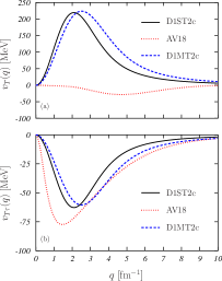
Figure 1: (Color online) Pure tensor (panel (a)) and tensor–isospin (panel (b)) terms of the D1ST2c and D1MT2c parameterizations used in this work as a function of the relative momentum of the interacting nucleon pair, compared with the analogous terms of the realistic interaction AV18 wir95 .

We show, in Fig. 1, the pure tensor, $v_{\rm T}$, and tensor-isospin, $v_{{\rm T}\tau}$, terms of the D1ST2c and D1MT2c forces as a function of the relative momentum of the two interacting nucleons, and we compare them with the analogous terms of the microscopic Argonne V18 (AV18) interaction wir95 . In this figure, the differences between the microscopic and, our, effective interactions become evident. The AV18 interaction has an actractive tensor-isospin term almost three times larger than the pure tensor term, which is again attractive. If the tensor-isospin terms of our effective interaction are similar to that of the AV18, the pure tensor terms are remarkably different. The sign is different, these terms are repulsive instead than actractive. In addition their size is much larger than that of the analogous AV18 term and also, in absolute value, of that of the tensor-isospin terms. Understanding the origin of these differences is an interesting topic, but we do not tackle it in this paper. We take for granted our effective interaction and we are interested in identifying eventual observables in charge-exchange excitations which are sensitive to the presence of the tensor force.

The first step of our calculations consists in constructing the s.p. basis by solving the HF equations with the bound-state boundary conditions at the edge of the discretization box. The technical details concerning the iterative procedure used to solve the HF equations for a density-dependent finite-range interaction can be found in Refs. co98b ; bau99 . When the stable solution, corresponding to the minimum of the binding energy, is reached, we construct the local Hartree and the non local Fock-Dirac potentials by using the s.p. wave functions lying below the Fermi surface. By using these potentials, we solve the HF equations also for those states above the Fermi surface. In this way, we generate a set of discrete bound states also in the positive energy region, which should be characterized by the continuum. The level density in the continuum region is strictly related to the size of the space integration box: the larger is the box the higher is the level density.

The second step of our calculations consists in solving the RPA secular equations by diagonalization. The explicit expressions of the $A^{J}$ and $B^{J}$ matrix elements in Eqs. (8) and (9) for Gogny interactions can be found in Refs. don14 ; don09 . The dimensions of the matrix to diagonalize are given by the sum of the $p\overline{n}$ and $n\overline{p}$ pairs that depends on the number of the s.p. states composing the configuration space.

In our approach, the stability of the RPA results depends on two parameters: the size of the integration box, and the maximum s.p. energy. We have chosen the values of these two parameters by controlling that the centroid energies of the electric giant dipole resonances in charge conserving RPA do not change by more than 0.5 MeV when either the box size or the maximum s.p. energies are increased. We have done calculations for the ⁴⁸Ca, ⁹⁰Zr  and ²⁰⁸Pb  nuclei. The most demanding calculations are those we carried out for the ²⁰⁸Pb  nucleus. In this nucleus, by using a box radius of 25 fm and an upper limit of s.p. energy of 100 MeV, we diagonalized matrices of dimensions of about 1300 $\times$ 1300.

Our HF+RPA calculations are fully self-consistent, we have used for the evaluation of the RPA excited states the same interaction adopted to generate the s.p. wave functions and energies, including the Coulomb and the spin-orbit channels. Of course, the former interaction is not active in charge-exchange excitations. These terms of the effective nucleon-nucleon interaction are usually neglected in RPA calculations, since the evaluation of their contribution, considered small as compared to that of the other terms of the interaction, is computationally quite heavy. Recently, we studied the relevance of these two terms of the interaction in charge conserving HF+RPA calculations don14 .

		D1M	D1MT2c	D1S	D1ST2c		exp
48Ca	$B/A$	8.590	8.614	8.690	8.632		8.667 aud03 ; audw
	$r_{n}$	3.550	3.552	3.586	3.597		–
	$r_{p}$	3.415	3.418	3.441	3.460		–
	$r_{c}$	3.525	3.528	3.548	3.557		3.451 $\pm$ 0.009 vri87
	$r_{n}-r_{p}$	0.135	0.134	0.145	0.097		–
90Zr	$B/A$	8.636	8.670	8.736	8.692		8.710 aud03 ; audw
	$r_{n}$	4.231	4.230	4.269	4.277		–
	$r_{p}$	4.179	4.177	4.209	4.217		–
	$r_{c}$	4.269	4.269	4.298	4.305		4.258$\pm$ 0.008 vri87
	$r_{n}-r_{p}$	0.052	0.053	0.060	0.060		0.09 $\pm$ 0.07 ray78
							0.07 $\pm$ 0.04 yak06
208Pb	$B/A$	7.830	7.815	7.889	7.801		7.867 aud03 ; audw
	$r_{n}$	5.505	5.514	5.554	5.570		$5.78^{+0.16}_{-0.18}$ abr12
	$r_{p}$	5.413	5.420	5.433	5.446		–
	$r_{c}$	5.480	5.488	5.498	5.512		5.503$\pm$ 0.002 vri87
	$r_{n}-r_{p}$	0.092	0.094	0.121	0.124		$0.083<r_{n}-r_{p}<0.111$ cla03
							0.19 $\pm$ 0.09 kra91

Table 2: Binding energies per nucleon, $B/A$, in MeV, and neutron, $r_{n}$, proton, $r_{p}$, and charge, $r_{c}$, rms radii, in fm, of ⁴⁸Ca, ⁹⁰Zr  and ²⁰⁸Pb  nuclei obtained in HF calculations by using the various interactions adopted in our work.

IV Results

In this section we show some results of our investigation of charge-exchange excitations of three nuclei: ⁴⁸Ca, ⁹⁰Zr  and ²⁰⁸Pb. We present results related to F, GT, SQ and SD excitations. First, we address our attention to the differences between the results obtained with and without the tensor force. Since the tensor effects are rather similar for the two types of forces considered, we show in the figures only the strength distributions obtained by using the D1M and D1MT2c interactions. In the tables we present global results of our calculations obtained with all the interactions considered.

As pointed out in the previous section, the first step of our approach is the generation of the s.p. configuration space for each nucleus considered by means of a HF calculation. We present in Table 2 some results of these calculations: the binding energies per nucleon, $B/A$, the neutron, $r_{n}$, proton, $r_{p}$, charge $r_{c}$, root mean square (rms) radii, and the neutron skin, $r_{n}-r_{p}$. The charge distributions used to extract the $r_{c}$ radii, have been obtained by folding the pointlike proton distributions with a dipole proton electromagnetic form factor. The use of more refined form factors changes the radius values of few parts on a thousand. The experimental values of the binding energies have been taken from Refs. aud03 ; audw and those of the charge radii from the compilation of Ref. vri87 . The empirical value of the ²⁰⁸Pb  neutron rms radius has been obtained by the parity violation electron scattering PREX experiment abr12 and those of the neutron skins from Refs. ray78 ; yak06 for ⁹⁰Zr, and cla03 ; kra91 for ²⁰⁸Pb.

The agreement with the available experimental data is, in general, very good. This is not surprising since the binding energies and rms radii are part of the set of data used in the fit procedure adopted to select the values of the parameters of the D1M and D1S forces cha07t . We observe that the inclusion of the tensor forces does not modify sensitively the values of these observables.

			D1M	D1MT2c	D1S	D1ST2c	exp
48Ca	$p$	$1f_{7/2}$	-9.83	-8.44	-9.90	-8.18	-9.45
	$\overline{n}$	$1f_{7/2}$	-9.33	-9.72	-9.48	-9.68	-9.94
90Zr	$p$	$1g_{9/2}$	-5.78	-4.45	-5.98	-4.36	-5.08
	$\overline{n}$	$1g_{9/2}$	-11.80	-12.10	-11.90	-12.02	-11.97
208Pb	$p$	$1h_{9/2}$	-3.33	-3.87	-3.56	-4.21	-3.71
	$\overline{n}$	$3p_{1/2}$	-8.94	-8.29	-7.85	-8.09	-7.37

Table 3: Energies, in MeV, of the s.p. states near the Fermi surfaces of ⁴⁸Ca  and ⁹⁰Zr  and ²⁰⁸Pb  nuclei. We present the energies of the first proton empty state ($p$), and that of the last neutron occupied state ($\overline{n}$). The experimental values have been taken from the compilation of Ref. firestone .

In Table 3, for each of the three nuclei considered, we show the s.p. energies of the last occupied neutron states and the first empty proton states. It is evident that the HF calculations done with D1M and D1S interactions generate ⁴⁸Ca  ground states which are unstable under beta decay, since the energies of the unoccupied proton $1f_{7/2}$ state are lower than those of the analogous, occupied, neutron state. This instability of the HF ground state against the beta decay is not present in the other nuclei. The inclusion of tensor terms solves this problem, as it is shown by the s.p. energies corresponding to the D1ST2c and D1MT2c forces given in the table. We point out that the parameters of these interactions have been chosen to reproduce other observables, i.e. the spin-orbit splitting of the $1f$ neutron states in ⁴⁰Ca  , ⁴⁸Ca  and ⁵⁶Ni, therefore this is a genuine prediction of our model.

		D1M	D1MT2c	D1S	D1ST2c		expected
48Ca	$m_{0}^{\rm F-}$	8.49	8.34	8.40	8.26
	$m_{0}^{\rm F+}$	0.49	0.34	0.40	0.26
	$\Delta_{\rm F}$	8.00	8.00	8.00	8.00		8.00
90Zr	$m_{0}^{\rm F-}$	10.59	10.41	10.49	10.33
	$m_{0}^{\rm F+}$	0.60	0.41	0.49	0.33
	$\Delta_{\rm F}$	9.99	10.00	10.00	10.00		10.00
208Pb	$m_{0}^{\rm F-}$	46.40	46.66	46.33	46.40
	$m_{0}^{\rm F+}$	2.60	2.66	2.33	2.40
	$\Delta_{\rm F}$	43.80	44.00	44.00	44.00		44.00

Table 4: The IAS sum rule values for F excitations in ⁴⁸Ca, ⁹⁰Zr  and ²⁰⁸Pb  nuclei. The RPA responses have been integrated up to the maximum energy of 250 MeV for ⁴⁸Ca, 200 MeV for ⁹⁰Zr and 150 MeV for ²⁰⁸Pb. The $\Delta_{\rm F}$ values in the columns labelled with the force name are obtained as the difference between $m_{0}^{\rm F-}$ and $m_{0}^{\rm F+}$, while the expected values are $N-Z$ (see Eq. (26)).

We start our discussion about the charge-exchange excitations by considering first the IAS resonance. The validity and the consistency of our RPA calculations can be verified by observing the exhaustion of the sum rules (26) whose values are given in Table 4. The good agreement with the expected values indicates that our configuration spaces are large enough to reach the numerical convergence of our calculations. As expected, in nuclei with neutron excess, the total strength carried by the T_-  excitation is much larger than that of the T₊  excitation.

The IAS resonances in the ⁴⁸Ca  and ⁹⁰Zr  nuclei are dominated by the neutron-proton transitions between the analog $1f_{7/2}$ states in ⁴⁸Ca, and $1g_{9/2}$ states in ⁹⁰Zr. In RPA calculations the IAS excitation presents a well isolated large peak which carries more than the 90% of the total strength. Also in ²⁰⁸Pb  the IAS strength distribution shows a single sharp peak, however the situation is more complicated since there are various particle-hole (p-h) excitations contributing to the main excitation. The energies of the IAS peak, $\omega^{\rm F-}_{\rm max}$, for each nucleus and interaction considered are compared in Table 5 with the experimental values extracted from Refs. bai80 ; and85 ; wak97 ; aki95 ; wak05 ; yak06 ; yak09 ; wak10 ; wak12 .

		D1M	D1MT2c	D1S	D1ST2c		exp
48Ca	$\omega^{\rm F-}_{\rm max}$	5.67	6.26	5.66	6.25		$7.17$ and85
		-0.50	1.28	-0.52	1.50		(IPM)
	$\omega^{\rm GT-}_{\rm max}$	11.64	9.90	12.38	10.17		10.5 and85
	$\omega^{\rm GT-}_{\rm cen}$	9.87	10.35	10.28	10.26		–
	$\omega^{\rm SD-}_{\rm cen}$	21.61	22.48	20.81	20.83		–
90Zr	$\omega^{\rm F-}_{\rm max}$	10.88	11.32	10.79	11.19		$12.0\pm 0.2$ bai80
		6.02	7.65	5.92	7.66		(IPM)
	$\omega^{\rm GT-}_{\rm max}$	17.36	15.64	17.93	15.80		15.6 $\pm$ 0.3 wak97 ; wak05
	$\omega^{\rm GT-}_{\rm cen}$	15.68	15.80	15.84	15.90		16.54 wak05
	$\omega^{\rm SD-}_{\rm cen}$	24.98	24.47	25.56	24.90		30.74 yak06
208Pb	$\omega^{\rm F-}_{\rm max}$	17.23	17.21	17.02	16.97		$18.83\pm 0.02$ aki95
		11.35	11.32	10.77	10.74		(IPM)
	$\omega^{\rm GT-}_{\rm max}$	20.99	18.89	21.12	18.56		$19.2\pm 0.2$ aki95
	$\omega^{\rm GT-}_{\rm cen}$	19.64	18.74	19.02	19.61		–
	$\omega^{\rm SD-}_{\rm cen}$	25.08	25.04	25.40	25.01		28.37 wak10 ; wak12

Table 5: Main peak, $\omega^{\alpha-}_{\rm max}$, and centroid, ${\omega}_{\rm cen}^{\alpha-}$, energies, in MeV, for the F, GT, and SD responses. In the case of the F transitions, also the IPM values of the peak energies are shown, in italic.

Only the RPA calculations can provide a realistic description of these IAS excitations. The excitation energies in a pure independent particle model (IPM) can be obtained as the difference between the energies of the neutron and proton analog s.p. states. For ⁴⁸Ca  and ⁹⁰Zr, these energies are those shown in Table 3. In the case of ²⁰⁸Pb, we considered the $\bar{n}(3p_{1/2})$ and $p(3p_{1/2})$ s.p. states. The IPM values obtained are shown for the three nuclei in Table 5 (in italic). We observe indeed that the IAS energies obtained in the IPM are extremely small with respect to those of the RPA, and they are even negative for ⁴⁸Ca  in the D1M and D1S cases, as we have pointed out above. This indicates that interactions and RPA correlations play an important role in the description of these excitations, even though they are not collective states, indeed their strength is concentrated in a single resonance largely dominated by the IPM p-h transition.

In ⁴⁸Ca  and ⁹⁰Zr  the inclusion of the tensor force increases the values of peak energy $\omega^{\rm F-}_{\rm max}$ in the correct direction to improve the description of the experimental value by about 0.5 and 0.4 MeV respectively. The effect of the tensor force is smaller and of opposite sign in the ²⁰⁸Pb  nucleus. Though the quality of the description of the experimental peak energies is not satisfactory, it is, however, similar to that obtained by self-consistent calculations carried out with Skyrme interactions col94 .

The role of the tensor force is more relevant in the GT excitations. We give in Table 5 the energies of the main peaks, $\omega^{\rm GT-}_{\rm max}$, and the centroid energies $\omega^{\rm GT-}_{\rm cen}$, of this type of excitation for the three nuclei and for all the interactions considered. In the left panels of Fig. 2 we present the $\Gamma_{1^{+}}^{{\rm GT}-}(\omega)$ strength distributions obtained with the D1M (red solid curves) and D1MT2c (blue dashed curves) interactions. In the figure, our discrete results have been folded with a Lorentz function of 1 MeV width. The arrows indicate the experimental values of the main peak energies and85 ; wak97 ; aki95 ; wak05 . The consistency and convergence of our calculations can be verified by observing the sum rule values given in Table 6. The results shown in this table indicate that the T_-  transitions carry the major part of the total sum rule.

		D1M	D1MT2c	D1S	D1ST2c		expected
48Ca	$m_{0}^{\rm GT-}$	24.74	24.64	24.57	24.47
	$m_{0}^{\rm GT+}$	0.74	0.71	0.57	0.64
	$\Delta_{\rm GT}$	24.00	23.93	24.00	23.83		24.00
90Zr	$m_{0}^{\rm GT-}$	31.10	30.92	30.92	30.72
	$m_{0}^{\rm GT+}$	1.12	0.99	0.92	0.82
	$\Delta_{\rm GT}$	29.98	29.93	30.00	29.90		30.00
208Pb	$m_{0}^{\rm GT-}$	137.33	135.97	136.91	134.92
	$m_{0}^{\rm GT+}$	5.38	5.26	4.96	4.90
	$\Delta_{\rm GT}$	131.95	130.71	131.95	130.02		132.00

Table 6: Sum rule for GT excitations in ⁴⁸Ca, ⁹⁰Zr  and ²⁰⁸Pb  nuclei. The $\Delta_{\rm GT}$ values in the columns labelled with the force name are obtained as the difference between $m_{0}^{\rm GT-}$ and $m_{0}^{\rm GT+}$, while the expected values are $3(N-Z)$ (see Eq. (27)). The values of the maximum excitation energies used to integrate the RPA responses are the same as those indicated in the caption of table 4.

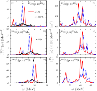
Figure 2: (color on line) Energy distributions of the $\Gamma_{1^{+}}^{{\rm GT}-}(\omega)$ (left panels), and $\Gamma_{1^{+}}^{{\rm SQ}-}(\omega)$ (right panels) strengths, as given by Eq. (15). The red solid curves have been obtained with the D1M interaction while the blue dashed curves with the D1MT2c force. The arrows indicate the experimental energies of the main peaks and85 ; wak97 ; aki95 ; wak05 ; wak10 ; wak12 . The black squares show the ⁴⁸Ca, ⁹⁰Zr and ²⁰⁸Pb experimental data, taken, respectively, from Refs. yak09 ; wak05 ; wak12 .

From Fig. 2 we observe that all the GT strength distributions present essentially two peaks. The smaller ones lie well below the experimental energy of the main peaks. The largest peaks obtained with the D1M interaction occur at energies close, slightly above, these experimental values. The use of the D1MT2c force, which includes the tensor terms, changes the position of these peaks, even though does not modify sensitively the values of the centroid energies, as it is shown in table 5. The tensor terms reduce the energy of the large peaks by 2-3 MeV and remarkably improve the agreement with the experimental data. These effects of the tensor force are similar to those found with Skyrme interactions bai11a . As seen in the panel (b) of the figure, our RPA results describe reasonably well the positions of the peaks but they miss completely the description of the experimental energy distribution of the strengths. This is not a specific problem of our implementation of the HF+RPA approach, but rather an intrinsic limit of the RPA that, by considering 1p-1h excitation only, does not include the spreading width. The experimental data for ⁹⁰Zr may contain the contribution of the excitation induced by the isovector spin monopole operator boh75 ; conde92 . The discussion done in Ref. wak97 indicates that the presence of this type of excitation is negligible in the data measured in the experiment at forward scattering angle, and for this reason we did not consider it. It is however a topic worth to be further investigated bes12 ; civ14 .

Using Skyrme interactions, Bai et al. bai09 showed that about 10% of the GT strength is moved above 30 MeV when the tensor terms are included in the RPA calculation. We have analyzed the strength distributions of our GT results and have found a similar effect though the shift of the strength is only 5%.

To make another comparison with the results of Ref. bai09 we have calculated the $\Gamma_{1^{+}}^{{\rm SQ}-}(\omega)$ strength distributions obtained with the SQ operator. In the right panels of Fig. 2 we show the results obtained with the D1M (red solid curves) and D1MT2c (blue dashed curves) forces. The basic effect of the tensor force is to move the strengths towards higher energies. The sizes of these shifts are much smaller than those found in Ref. bai09 ; sag14 for the Skyrme interaction.

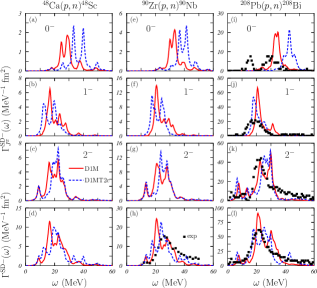
Figure 3: (color on line) Energy distributions of the $\Gamma_{J^{\pi}}^{{\rm SD}-}(\omega)$ and $\Gamma^{{\rm SD}-}(\omega)$ strengths for ⁴⁸Ca  (left panels), ⁹⁰Zr  (central panels) and ²⁰⁸Pb  (right panels) nuclei. The red solid curves have been obtained with the D1M interaction while the blue dashed curves with the D1MT2c force. The squares indicate the experimental data of Ref. yak06 , for ⁹⁰Zr, and of Refs. wak10 ; wak12 , for ²⁰⁸Pb.

In Fig. 3 we show the $\Gamma_{J^{\pi}}^{{\rm SD}-}(\omega)$ strength distributions for ⁴⁸Ca  (left panels), ⁹⁰Zr  (central panels) and ²⁰⁸Pb  (right panels) nuclei. The results obtained with the D1M (red solid curves) and the D1MT2c (blue dashed curves) interactions are shown. These excitations imply the superposition of the responses of three different multipoles, the $0^{-}$ (panels (a), (e) and (i)), $1^{-}$ (panels (b), (f) and (j)), and $2^{-}$ (panels (c), (g) and (k)). Our calculations produce discrete results for each multipole considered even above the nucleon emission threshold. Since the experimental strengths of Refs. yak06 ; wak10 ; wak12 are above this threshold, a comparison with them requires the sum of the three responses. Because of the large numbers of peaks in this excitation region we fold our discrete results with a Lorentz function of 2MeV width. This procedure produces smooth continuous strength distributions which we sum for each value of the excitation energy, as indicated in Eq. (20), to obtain the total strength $\Gamma^{{\rm SD}-}(\omega)$ (panels (d), (h) and (l)).

		D1M	D1MT2c	D1S	D1ST2c		exp
48Ca	$m_{0}^{\rm SD-}$	137.60	141.52	140.08	145.68		–
	$m_{0}^{\rm SD+}$	51.96	53.64	51.81	56.39		–
	$\Delta_{\rm SD}$	85.64	87.88	88.27	89.29		–
expected	$\Delta_{\rm SD}$	85.68	85.67	88.27	88.89		–
90Zr	$m_{0}^{\rm SD-}$	276.42	279.53	281.51	285.41		$271\pm 14$
	$m_{0}^{\rm SD+}$	135.37	136.42	136.50	135.41		$124\pm 11$
	$\Delta_{\rm SD}$	141.05	143.11	145.01	150.00		$147\pm 13$
expected	$\Delta_{\rm SD}$	140.74	140.91	145.09	145.61		–
208Pb	$m_{0}^{\rm SD-}$	1176.40	1188.38	1210.90	1204.92		–
	$m_{0}^{\rm SD+}$	170.45	150.75	165.46	148.45		–
	$\Delta_{\rm SD}$	1005.95	1037.63	1045.44	1056.47		–
expected	$\Delta_{\rm SD}$	1013.98	1018.47	1050.14	1057.90		–

Table 7: Sum rule values, in fm² for SD excitations in ⁴⁸Ca, ⁹⁰Zr  and ²⁰⁸Pb  nuclei. The $\Delta_{\rm SD}$ values in the columns labelled with the force name are obtained as the difference between $m_{0}^{\rm SD-}$ and $m_{0}^{\rm SD+}$. The expected $\Delta_{\rm SD}$ values have been calculated by using Eq. (28). The experimental data for ⁹⁰Zr  are taken from Ref. yak06 . The values of the maximum excitation energies used to integrate the RPA responses are the same as those indicated in the caption of table 4.

The consistency of our calculations can be verified by observing the results shown in Table 7, i.e. the values of the, positive and negative, zero-th energy moments (21) and of the SD sum rules. These last values must be compared with those shown in Table 2 which have been obtained by using the expression (28). We observe a maximal deviation of about 5%. In the case of the ⁹⁰Zr  nucleus we show the experimental values of Ref. yak06 , and we observe the general good agreement of our calculations within the range of the experimental uncertainties.

There are common characteristics related to the results shown in Fig. 3. In all the cases considered, the strength of the $0^{-}$ excitations is smaller than those of the $1^{-}$ and $2^{-}$ modes which are of similar size. Furthermore, the main peaks of the $0^{-}$ responses are located at higher energies than the peaks of the $1^{-}$ and $2^{-}$ which almost overlap.

Also in these charge-exchange excitations the $0^{-}$ state is extremely sensitive to the tensor force as it has been observed for the charge conserving case blo68 ; ang11 . As seen in panels (a), (e) and (i) of Fig. 3, the tensor force shifts at higher energies the strength of this excitation mode. The inclusion of the tensor term is even worsening the agreement with the experimental strength distribution disentangled in the data of Refs. wak10 ; wak12 for ²⁰⁸Pb  (see panel (i)).

At variance with the large effects on the $0^{-}$ excitations, the tensor term does not remarkably modifies the strength distributions of the other two SD resonances. Since the strengths of these resonances are larger than those of the $0^{-}$ excitations, the total response is scarcely affected by the presence of the tensor force (see panels (d), (h) and (l)). The size of these effects can be estimated by the small changes in the centroid energies shown in Table 5. The general trend of these results is analogous to that of the results of Ref. bai10 , even though the size of the effects is smaller.

In the second part of the section we analyze in more detail the role of the tensor force which affects our model in the HF calculations, where it modifies the s.p. wave functions and energies which are input of the RPA, and directly in the RPA. In order to disentangle these two effects, we have carried out HF and RPA calculations by switching on and off the tensor terms of the interaction. We label as [0,0] the results obtained without tensor force in both HF and RPA calculations. These do not correspond to the results obtained with the D1M and D1S forces previously presented, since the values of the spin-orbit terms of the D1MT2c and D1ST2c interactions are used. We label [1,0] the results obtained by using the tensor force in HF calculations only, and [1,1] those where the tensor force has been used in both HF and RPA calculations. These last results are those previously shown. In addition, since our tensor interaction contains two terms, see Eq. (31), we have investigated separately their relevance in the RPA calculations. We have labelled our results [1,t] or [1,ti] if only the pure tensor or the tensor-isospin terms, respectively, are included in the RPA calculations. In these two cases, the complete tensor interaction is considered in HF.

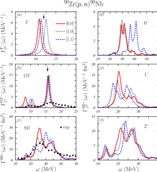
Figure 4: (color on line) Energy distributions of the T_-  responses of ⁹⁰Zr  calculated with the D1MT2c interaction. We show in panels (a), (b) and (c) the strengths $\Gamma_{0^{+}}^{{\rm F}-}(\omega)$, $\Gamma_{1^{+}}^{{\rm GT}-}(\omega)$ and $\Gamma^{{\rm SD}-}(\omega)$, respectively. The SD strengths for the 0^-, 1^- and 2^- multipoles are shown in the right panels. The red solid lines labeled [0,0] indicate the results obtained without tensor terms in both HF and RPA calculations; those labeled [1,0] (black dotted curves) the results obtained by considering the tensor force only in the HF calculations, and, finally, those identified with [1,1] (blue dashed) have been obtained by considering the tensor force in both HF and RPA calculations. The arrows indicate the experimental energies of the main peaks for the SD (Ref.bai80 ) and GT (Refs. wak97 ; wak05 ) excitations. Experimental data (black solid squares) are from Ref. wak05 for GT strength and from Ref. yak06 for SD one.

We conducted this study in all the three nuclei considered up to now, and with both the D1MT2c and D1ST2c interactions. However, since we observed rather similar effects, we present in Figs. 4 and 5 only the results obtained in ⁹⁰Zr  with the D1MT2c interaction. In Fig. 4, we show the T_-  strength distributions obtained for the F (panel (a)) and GT (panel (b)) transitions. The results of panel (a) indicate that the IAS is sensitive to the changes of s.p. states and energies due to the presence of the tensor force in HF calculations. These modifications move the resonance peak towards higher energies. This is compensated by a shift in the opposite direction when the tensor force is included in the RPA calculation.

An analogous, but much smaller, sensitivity to the effect of the tensor channel is found in the largest peak of the GT response (see panel (b)). Instead, the presence of the tensor force noticeably affects the smaller peak. Its inclusion in HF calculations generates a remarkable shift of the peak to higher energies. The use of the tensor force in the RPA calculations produces a smaller shift in the same direction.

These last results can be understood in terms of the so-called Otsuka effect ots05 present in HF calculations with the tensor force. This effect is the main responsible of the global tensor effect we have observed in the GT responses. In HF calculations the tensor force between an occupied neutron state with angular momentum $j=l+1/2$ increases the energy of the proton $j=l+1/2$ s.p. state and lowers that of the proton $j=l-1/2$ states. This effect decreases the energy difference between spin-orbit partners. An analogous effect of different sign occurs with the neutron $j=l-1/2$ states. In nuclei where all the s.p. spin-orbit partner states are occupied the two effects compensate. This is not the case for ⁹⁰Zr  where the last occupied neutron state is the $\bar{n}(1g_{9/2})$. The inclusion of the tensor term in HF increases the s.p. energy of the proton $p(1g_{9/2})$ state by 1.3 MeV, and reduces that of the proton $p(1g_{7/2})$ state by 1.7 MeV. The low-lying peak observed in panels (b) of Figs. 2 and 4 is dominated by the $\bar{n}(1g_{9/2})-p(1g_{9/2})$ p-h transition, while the $\bar{n}(1g_{9/2})-p(1g_{7/2})$ is the main configuration in the other peak. Therefore the energy of the first peak is increased, while that of the second one is reduced and the energy difference between the two GT peaks decreases. No additional modifications of the situation occur, since the tensor force, in this case, has very small effects on the RPA calculations. An analogous trend is observed in ⁴⁸Ca  where the states involved are the proton $p(1f_{7/2})$ and $p(1f_{5/2})$ s.p. states interacting with the neutron $\bar{n}(1f_{7/2})$. This effect explains also the upward shift of the IAS response, (see panel (a) of Fig. 4), when the tensor force is included.

In the right panels of Fig. 4 we show the $\Gamma_{J^{\pi}}^{{\rm SD}-}(\omega)$ responses for each multipole considered and in panel (c) the total $\Gamma^{{\rm SD}-}(\omega)$ strength. The effects of the tensor force are rather small in both HF and RPA calculations for $1^{-}$ and $2^{-}$ responses. Since these are the dominant strengths, also the total response is practically unaffected by the inclusion of the tensor term. Different is the situation for the $0^{-}$ state. While there are not effects when the tensor is included in HF calculations, the RPA responses show a large energy shift.

		D1MT2c					D1ST2c
		[1,0][0,0]	[1,t][1,0]	[1,ti][1,0]	[1,1][1,0]		[1,0][0,0]	[1,t][1,0]	[1,ti][1,0]	[1,1][1,0]
48Ca	$s^{{\rm F}-}$	1.96	-1.07	-0.28	-1.37		2.12	-1.17	-0.33	-1.52
	$s^{{\rm GT}-}$	0.97	0.49	0.12	0.51		1.00	0.51	0.11	0.52
	$s^{{\rm SD}-}$	0.62	0.20	0.05	1.15		0.61	0.21	0.04	1.12
	$s_{0^{-}}^{{\rm SD}-}$	0.35	8.03	1.01	8.21		0.27	8.18	0.75	8.01
	$s_{1^{-}}^{{\rm SD}-}$	0.56	-1.56	-0.38	-2.17		0.54	-1.54	-0.38	-2.21
	$s_{2^{-}}^{{\rm SD}-}$	0.72	1.19	0.29	1.35		0.74	1.21	0.23	1.34
90Zr	$s^{{\rm F}-}$	1.79	-1.01	-0.26	-1.29		1.91	-1.09	-0.30	-1.42
	$s^{{\rm GT}-}$	0.87	0.44	0.08	0.50		0.88	0.46	0.13	0.48
	$s^{{\rm SD}-}$	0.43	0.07	0.00	0.88		0.15	0.11	0.01	0.73
	$s_{0^{-}}^{{\rm SD}-}$	0.22	5.85	1.06	7.30		0.15	7.00	0.92	7.23
	$s_{1^{-}}^{{\rm SD}-}$	0.42	-1.54	-0.38	-2.10		0.39	-1.49	-0.34	-2.16
	$s_{2^{-}}^{{\rm SD}-}$	0.48	0.87	0.09	0.95		0.47	0.89	0.10	0.84
208Pb	$s^{{\rm F}-}$	0.04	-0.03	0.00	-0.03		0.06	-0.03	-0.01	-0.04
	$s^{{\rm GT}-}$	0.19	0.41	0.09	0.36		0.06	0.40	0.09	0.33
	$s^{{\rm SD}-}$	0.20	0.43	0.06	0.71		0.38	0.43	0.04	0.78
	$s_{0^{-}}^{{\rm SD}-}$	0.32	7.99	1.56	9.04		0.24	8.14	1.49	7.23
	$s_{1^{-}}^{{\rm SD}-}$	0.23	-1.86	-0.48	-2.42		0.18	-1.81	-0.47	-2.40
	$s_{2^{-}}^{{\rm SD}-}$	0.14	0.80	0.10	0.92		0.11	0.82	0.08	0.97

Table 8: Energy differences, in MeV, between centroid energies calculated in different manners, as defined by Eq. (34), for all the nuclei, interactions and transitions considered in our work.

As we have already pointed out, we obtain similar results for the other two nuclei and for the D1ST2c interaction. This can be seen in Table 8 where we summarize the shifts between the centroid energies obtained for different calculations by showing the values of

$$s^{\alpha-}([a,b][c,d])\,=\,\omega_{\rm cent}^{\alpha-}[a,b]\,-\,\omega_{\rm cent}^{\alpha-}[c,d]\,.$$ (34)

The letters indicated in the brackets are 0, 1, t or ti according to the use of the tensor interaction in HF and RPA calculations (see above). The shifts $s_{J^{\pi}}^{{\rm SD}-}([a,b][c,d])$ calculated for the individual multipolarities in the case of the SD transitions can be defined in an analogous way.

Coming back to the situation described above, the centroid energy in the case of the multipolarity $0^{-}$ in the T_-  SD transition is shifted by 7.30 MeV in ⁹⁰Zr, as indicated by the [1,1][1,0] column for D1MT2c interaction in Table 8. In ⁴⁸Ca  and ²⁰⁸Pb, $s_{0^{-}}^{{\rm SD}-}([1,1][1,0])$ is 8.21 and 9.04 MeV, respectively. These values are much larger than those found for the other multipolarities and for the total SD transition. As it is shown in the table, we find a similar trend in all the nuclei considered and for both D1MT2c and D1ST2c interactions. This is a genuine effect of the tensor force.

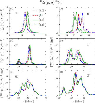
Figure 5: (color on line) The same as in Fig. 4. In this case, all the calculations have been carried out by including tensor force in the HF calculations. The [1,0] black dotted and [1,1] blue dashed lines are the same as those of Fig. 4, and have been included here to facilitate the comparison with the other results. The [1,t] red dashed-dotted curves have been obtained by including only the pure tensor force in RPA calculations, while those obtained by including only the tensor-isospin force are named [1,ti] (green solid curves).

For the ⁹⁰Zr and the D1MT2c force, we show in Fig. 5 the comparison between the results obtained with and without the two tensor terms in the RPA calculations. The corresponding shifts of the centroid energies are presented in Table 8. These calculations have been carried out by including the full tensor force in HF.

In general, the sensitivity to the pure tensor term is much larger than that to the tensor-isospin one. This can be deduced from the fact that the results of the [1,0] (black dotted curves) and [1,ti] (green solid curves) calculations are rather close in all the cases, while the consideration of the pure tensor term in the RPA calculations ([1,t] red dashed-dotted curves) produces results very similar to the complete [1,1] calculations (blue dashed curves). As a consequence, the main effect of the tensor interaction is essentially due to the presence of the pure tensor term. An analogous effect is observed in the F excitation.

V Summary and conclusions

In this paper, we have presented results of charge-exchange responses calculated within the HF+RPA framework with finite-range interactions. These are parameter free calculations, since no part of the interactions has been modified. Even though we have considered only doubly magic nuclei, however these interactions can be used also to describe pairing effects in open shell nuclei mar14 . Our approach is fully self-consistent since all the terms of the interaction used in the HF calculations have been considered in the RPA, even the spin-orbit term which is usually neglected in the latter calculations.

We have used two well tested parameterizations of the Gogny interaction, the D1S and D1M forces. We have also considered two other interactions containing tensor terms. These last interactions have been constructed by adding to the original D1M and D1S forces a tensor and a tensor-isospin terms. The parameters defining the tensor force have been chosen following the procedure indicated in Ref. gra13 which implies only a change in the strength of the spin-orbit force. We have investigated the role of the tensor force by comparing the results obtained with the original Gogny forces and those with the new interactions.

We first remark that the HF calculations done with the original Gogny forces generate a ⁴⁸Ca  ground state unstable for beta decay. The interactions with tensor force stabilize the situation.

Our study of the IAS excitations shows that the IPM is unable to predict reasonable excitation energies, while the RPA results describe them much better. These excitations are characterized by a single peak which is not very sensitive to the presence of the tensor force. This small effect is due to a cancellation of two sizable effects which work in opposite directions. The inclusion of the tensor force in HF calculations changes the s.p. energies and, consequently, we obtain peak positions which are 2 or 3 MeV larger. When the tensor force is included in our RPA calculations we obtain an opposite effect which essentially compensates the previous shift.

We observe remarkable effects of the tensor force on the GT responses, effects that help in improving the description of the experimental data. Our GT responses are characterized by two main peaks generated by the transitions of the excess neutrons from their last occupied s.p. level, with orbital angular momentum $l$, to the empty proton levels with the same orbital angular momentum. In this case, the major effect of the tensor force is the reduction of the energy difference between the proton s.p. levels in HF calculations. This implies a reduction of the difference between the energies of the two GT peaks, since the tensor force does not produce relevant effects in the RPA level.

The results obtained for the SD excitation indicate that only the $0^{-}$ multipole is very sensitive to the presence of the tensor force, and this happens essentially in the RPA calculation, contrary to what we have observed for the GT resonances. In ²⁰⁸Pb  it has been possible to disentangle the experimental SD strength attributed to the $0^{-}$ excitation, and we found that the inclusion of the tensor term is even worsening the agreement with the experimental data. We observe that the tensor effects on the SD multipole decrease with increasing value of the angular momentum. This behavior is similar to that found in Ref. bai10 .

Our investigation indicates that the tensor effects we have identified are mainly due to the pure tensor term of the interaction, while the role of the tensor-isospin term is smaller.

The results found in the present investigation give a reasonable description of the experimental excitation energies but fail in describing the width of the resonances. This is a problem related to the intrinsic limit of the RPA which considers only 1p-1h excitations, and it is present also in the description of charge conserving excitations. The inclusion of two particle-two hole excitations dro90 ; kam04 , or particle-vibration coupling col94 improves the agreement with the experimental strength distributions.

We have studied the validity of our model by comparing our results with the experimental data and with the results of other self-consistent approaches. We conclude that the accuracy of modern data needs the use of an effective nucleon-nucleon interaction which contains tensor terms. A better tuning of these terms of the effective interaction is required to apply our model in experimentally unknown regions of the nuclear chart.

Appendix A Transition matrix elements

The s.p. transition operators defined in Eq. (14) can be expressed as the product of a term depending only on the radial coordinate of the $i$-th particle, another term depending on the angular coordinates and the spin of this particle and a third, isospin dependent, term $\tau_{\pm}(i)=2t_{\pm}(i)$:

$${\eta}^{\alpha\pm}_{J^{\pi},M}(i)\,=\,\Phi_{\alpha}(r_{i})\,{\cal B}^{\alpha}_{J,M}(i)\,t_{\pm}(i)\,.$$ (35)

According to Eqs. (14) and (16)-(19) we have

$$\Phi_{\rm F}(r_{i}) = 1\,,$$ (36)

$$\Phi_{\rm GT}(r_{i}) = 1\,,$$ (37)

$$\Phi_{\rm SQ}(r_{i}) = r_{i}^{2}\,,$$ (38)

$$\Phi_{\rm SD}(r_{i}) = r_{i}\,,$$ (39)

and

$${\cal B}^{\rm F}_{0,0}(i) = 1\,,$$ (40)

$${\cal B}^{\rm GT}_{1,M}(i) = \sqrt{4\pi}\,[Y_{0}(i)\otimes\mbox{\boldmath$\sigma$}(i)]^{1}_{M}\,,$$ (41)

$${\cal B}^{\rm SQ}_{1,M}(i) = [Y_{2}(i)\otimes\mbox{\boldmath$\sigma$}(i)]^{1}_{M}\,,$$ (42)

$${\cal B}^{\rm SD}_{J,M}(i) = [Y_{1}(i)\otimes\mbox{\boldmath$\sigma$}(i)]^{J}_{M}\,.$$ (43)

Then, the reduced s.p. matrix elements of Eq. (15) can be written as

$$\langle a\|{\eta}^{\alpha\pm}_{J^{\pi}}\|b\rangle\,=\,\frac{1}{2}\int{\rm d}r_{i}\,r_{i}^{2}\,R^{*}_{a}(r_{i})\,R_{b}(r_{i})\,\Phi_{\alpha}(r_{i})\,\langle l_{a}\frac{1}{2}j_{a}\|{\cal B}^{\alpha}_{J}(i)\|l_{b}\frac{1}{2}j_{b}\rangle\,\langle\frac{1}{2}t_{a}|\tau_{\pm}|\frac{1}{2}t_{b}\rangle\,,$$ (44)

where $R_{a}(r)$ and $R_{b}(r)$ indicate the radial part of the s.p. wave functions, $l_{a}$ and $l_{b}$ are the orbital angular momenta of the s.p. states and $t_{a}$ and $t_{b}$ are the third components of their isospin. In the above equation we have dropped the dependence on $M$ since we have already applied the Wigner-Eckart theorem.

For the F operator, we have

$$\langle l_{a}\frac{1}{2}j_{a}\|{\cal B}^{\rm F}_{0}(i)\|l_{b}\frac{1}{2}j_{b}\rangle\,=\,\hat{j}_{a}\,\delta_{l_{a},l_{b}}\,\delta_{j_{a},j_{b}}\,,$$ (45)

where we have used the symbol $\hat{j}_{a}=\sqrt{2j_{a}+1}$. For the other operators, in case of natural parity excitations, implying $L=J$, we can write

$$\langle l_{a}\frac{1}{2}j_{a}\|[Y_{L}(i)\otimes\mbox{\boldmath$\sigma$}(i)]^{J}\|l_{b}\frac{1}{2}j_{b}\rangle\,=\,(-1)^{l_{a}}\,\xi(l_{a}+l_{b}+J)\,\frac{\hat{j}_{a}\,\hat{j}_{b}\,\hat{J}}{\sqrt{4\pi}}\,\left(\begin{array}[]{ccc}j_{a}&j_{b}&J\\ 1/2&1/2&-1\end{array}\right)\,.$$ (46)

For unnatural parity excitations, with $L=J+s$ with $s=\pm 1$, we write

$$\langle l_{a}\frac{1}{2}j_{a}\|[Y_{L}(i)\otimes\mbox{\boldmath$\sigma$}(i)]^{J}\|l_{b}\frac{1}{2}j_{b}\rangle = (-1)^{l_{a}+l_{b}+j_{b}+\frac{1}{2}}\,\xi(l_{a}+l_{b}+J+1)\,\frac{\hat{j}_{a}\hat{j}_{b}}{\sqrt{4\pi}}$$ (49)

$$\frac{\chi_{a}+\chi_{b}+sJ+\delta(s,1)}{\sqrt{J+\delta(s,1)}}\,\left(\begin{array}[]{ccc}j_{a}&j_{b}&J\\ 1/2&-1/2&0\end{array}\right)\,,$$

where $\xi(n)=1$ or 0 if $n$ is even or odd, respectively, and $\chi_{a}=(l_{a}-j_{a})(2j_{a}+1)$.

Finally, the isospin matrix element of Eq. (44) is given by

$$\langle\frac{1}{2}t_{a}|\tau_{+}|\frac{1}{2}t_{b}\rangle = \delta_{a,n}\,\delta_{b,p}\,,$$ (50)

$$\langle\frac{1}{2}t_{a}|\tau_{-}|\frac{1}{2}t_{b}\rangle = \delta_{a,p}\,\delta_{b,n}\,.$$ (51)

- (1) F. Osterfeld, Rev. Mod. Phys. 64 (1992) 491.
- (2) M. Ichimura, H. Sakai, T. Wakasa, Prog. Part. Nucl. Phys. 56 (2006) 446.
- (3) Y. Fujita, B. Rubio, W. Gelletly, Prog. Part. Nucl. Phys. 66 (2011) 549.
- (4) M. Arnould, S. Goriely, K. Takahashi, Phys. Rep. 450 (2007) 97.
- (5) J. Speth, J. Wambach, Theory of giant resonances. in Electric and magnetic giant resonances in nuclei, J. Speth ed., World Scientific, Singapore, 1991.
- (6) J. A. Halbleib, R. A. Sorensen, Nucl. Phys. A 98 (1967) 542.
- (7) A. M. Lane, J. Martorell, Ann. Phys. (N.Y.) 129 (1980) 273.
- (8) N. Auerbach, A. Klein, N. V. Giai, Phys. Lett. B 106 (1981) 347.
- (9) N. Auerbach, A. Klein, Nucl. Phys. A 395 (1983) 77.
- (10) I. Hamamoto, H. Sagawa, Phys. Rev. C 62 (2000) 024319.
- (11) S. Fracasso, G. Colò, Phys. Rev. C 76 (2007) 044307.
- (12) C. L. Bai, H. Sagawa, H. Q. Zhang, X. Z. Zhang, G. Colò, F. R. Xu, Phys. Lett. B 675 (2009) 28.
- (13) C. L. Bai, H. Q. Zhang, X. Z. Zhang, F. R. Xu, H. Sagawa, G. Colò, Phys. Rev. C 79 (2009) 041301(R).
- (14) C. L. Bai, H. Q. Zhang, H. Sagawa, X. Z. Zhang, G. Colò, F. R. Xu, Phys. Rev. Lett. 105 (2010) 072501.
- (15) C. L. Bai, et al., Phys. Rev. C 83 (2011) 054316.
- (16) C. L. Bai, H. Sagawa, G. Colò, H. Q. Zhang, X. Z. Zhang, Phys. Rev. C 84 (2011) 044329.
- (17) F. Minato, C. L. Bai, Phys. Rev. Lett. 110 (2013) 122501.
- (18) D. R. Bes, O. Civitarese, J. Suhonen, Phys. Rev. C 86 (2012) 024314.
- (19) O. Civitarese, J. Suhonen, Phys. Rev. C 89 (2014) 044319.
- (20) J. F. Berger, M. Girod, D. Gogny, Comp. Phys. Commun. 63 (1991) 365.
- (21) S. Goriely, S. Hilaire, M. Girod, S. Péru, Phys. Rev. Lett. 102 (2009) 242501.
- (22) M. Grasso, M. Anguiano, Phys. Rev. C 88 (2013) 054328.
- (23) A. R. Edmonds, Angular momentum in quantum mechanics, Princeton University Press, Princeton, 1957.
- (24) C. Gaarde, J. S. Larsen, M. N. Harakeh, S. V. van der Werf, M. Igarashi, A. Müller-Arnke, Nucl. Phys. A 334 (1980) 248.
- (25) M. Anguiano, M. Grasso, G. Co’, V. De Donno, A. M. Lallena, Phys. Rev. C 86 (2012) 054302.
- (26) N. Onishi, J. W. Negele, Nucl. Phys. A 301 (1978) 336.
- (27) R. B. Firestone, http://isotopes.lbl.gov/toi.html.
- (28) R. B. Wiringa, V. G. J. Stoks, R. Schiavilla, Phys. Rev. C 51 (1995) 38.
- (29) G. Co’, A. M. Lallena, Nuovo Cimento A 111 (1998) 527.
- (30) A. R. Bautista, G. Co’, A. M. Lallena, Nuovo Cimento A 112 (1999) 1117.
- (31) V. De Donno, G. Co’, M. Anguiano, A. M. Lallena, Phys. Rev. C 89 (2014) 014309.
- (32) V. De Donno, G. Co’, C. Maieron, M. Anguiano, A. M. Lallena, M. Moreno-Torres, Phys. Rev. C 79 (2009) 044311.
- (33) G. Audi, A. H. Wapstra, C. Thibault, Nucl. Phys. A 729 (2003) 337.
- (34) http://ie.lbl.gov/toi2003/masssearch.asp.
- (35) H. de Vries, C. de Jagger, C. de Vries, At. Data Nucl. Data Tables 36 (1987) 495.
- (36) S. Abrahamayn, et. al. P.R.E.X. coll., Phys. Rev. Lett. 108 (2012) 112502.
- (37) L. Ray, G. W. Hoffmann, G. S. Blanpied, W. R. Coker, R. P. Liljestrand, Phys. Rev. C 18 (1978) 1756.
- (38) K. Yako, H. Sagawa, H. Sakai, Phys. Rev. C 74 (2006) 051303(R).
- (39) K. Yako, et al., Phys. Rev. Lett. 103 (2009) 012503.
- (40) B. C. Clark, L. J. Kerr, S. Hama, Phys. Rev. C 67 (2003) 054605.
- (41) A. Krasznahorkay, et al., Phys. Rev. Lett. 66 (1991) 1287.
- (42) F. Chappert, Nouvelles paramétrisation de l’interaction nucléaire effective de gogny, Ph.D. thesis, Université de Paris-Sud XI (France), http://tel.archives-ouvertes.fr/tel-001777379/en/ (2007).
- (43) D. E. Bainum, J. Rapaport, C. D. Goodman, D. J. Horen, C. C. Foster, M. B. Greenfield, C. A. Goulding, Phys. Rev. Lett. 44 (1980) 1751.
- (44) B. D. Anderson, et al., Phys. Rev. C 31 (1985) 1161.
- (45) T. Wakasa, et al., Phys. Rev. C 55 (1997) 2909.
- (46) H. Akimune, et al., Phys. Rev. C 52 (1995) 604.
- (47) T. Wakasa, M. Ichimura, H. Sakai, Phys. Rev. C 72 (2005) 067303(R).
- (48) T. Wakasa, arxiv:1004.5220[nucl-ex].
- (49) T. Wakasa, et al., Phys. Rev. C 85 (2012) 064606.
- (50) G. Colò, N. Van Giai, P. F. Bortignon, R. A. Broglia, Phys. Rev. C 50 (1994) 1496.
- (51) A. Bohr, B. R. Mottelson, Nuclear structure, vol. II, Benjamin, New York, 1975.
- (52) H. Condé, et al., Nucl. Phys. A 545 (1992) 785.
- (53) C. L. Bai, et al., Phys. Lett. B 675 (2009) 28.
- (54) H. Sagawa, G. Colò, arxiv:1401.6691 [nucl-th].
- (55) J. Blomqvist, A. Molinari, Nucl. Phys. A 106 (1968) 545.
- (56) M. Anguiano, G. Co’, V. De Donno, A. M. Lallena, Phys. Rev. C 83 (2011) 064306.
- (57) T. Otsuka, T. Suzuki, R. Fujimoto, H. Grawe, Y. Akaishi, Phys. Rev. Lett. 95 (2005) 232502.
- (58) M. Martini, S. Péru, S. Goriely, arxiv:1404.1493 [nucl-th].
- (59) S. Drożdż, S. Nishizaki, J. Speth, J. Wambach, Phys. Rep. 197 (1990) 1.
- (60) S. Kamerdzhiev, J. Speth, G. Tertychny, Phys. Rep. 393 (2004) 1.