Chemical Evolution on the Scale of Clusters of Galaxies: A Conundrum?

Abstract

The metal content of clusters of galaxies and its relation to their stellar content is revisited making use of a cluster sample for which all four basic parameters are homogeneously measured within consistent radii, namely core-excised mass-weighted metallicity plus total, stellar and ICM masses. For clusters of total mass $M_{500}\simeq 10^{14}\,\hbox{$M_{\odot}$}$ nice agreement is found between their iron content and what expected from empirical supernova yields. For the same clusters, there also appears to be at least as much iron in the intracluster medium (ICM) as there is still locked into stars (i.e., the ICM/stars metal share is about unity). However, for more massive clusters the stellar mass fraction appears to drop substantially without being accompanied by a drop in the ICM metallicity, thus generating a major tension with the nucleosynthesis expectation and inflating the metal share to extremely high values (up to $\sim 6$). Various possible solutions of this conundrum are discussed, but are all considered either astrophysically implausible, or lacking an independent observational support. For this reason we still entertain the possibility that even some of the best cluster data may be faulty, though we are not able to identify any obvious bias. Finally, based on the stellar mass-metallicity relation for local galaxies we estimate the contribution of galaxies to the ICM enrichment as a function of their mass, concluding that even the most massive galaxies must have lost a major fraction of the metals they have produced.

1 Introduction

Clusters of galaxies are the largest bound structures in the Universe, and have been often regarded as possibly being the best example of a closed-box system, i.e., a system in which all the actors are present from the beginning to the end (e.g., White et al. 1993). This is equivalent to assume that present-day clusters contain, together with their dark matter, all the baryons in their cosmic share that have contributed to star formation, all the stars that have formed out of them and all the metals produced by the successive stellar generations. This assumes that the baryonic fraction of clusters is equal to the cosmic ratio, $\Omega_{\rm b}/\Omega_{\rm m}\simeq 0.165$ (Komatsu et al., 2009), an hypothesis that can be subject to observational test, and appeared to be verified at least for the richest clusters (Gonzalez, Zaritzky & Zabludoff, 2007; Pratti et al., 2009; Andreon, 2010; Leauthaud et al., 2012). This assumption clearly fails at least for groups and low-mass clusters with mass less than $\sim 10^{13}\,\hbox{$M_{\odot}$}$, whose gas content can be much lower than the cosmic share, indicating that baryons may have been lost by these system or never incorporated in them (e.g., Renzini et al. 1993; McGaugh et al. 2010).

To the extent that the closed box assumption is close to reality, clusters of galaxies can offer a unique opportunity to study chemical evolution on the largest scale for which the census of all the mentioned components is virtually complete, hence allowing us to obtain an empirical measure of the chemical yield(s) ($y$) and the fraction of cosmic baryons turned into stars, i.e., the efficiency of galaxy formation.

In this paper we revisit these issues using updated cluster data that we consider of the best quality for our purposes, i.e., for which total, stellar and ICM mass and metallicity have been homogeneously measured within consistent radii. The paper is organized as follows: in Section 2 we summarize the basic understanding of cluster chemistry prior of the newer data presented in Section 3, which are then elaborated in Section 4. Section 5 expands on the implications of the new results which appear to pose new challenges, an apparent conundrum where in the most massive clusters there appears to be much more iron than the cluster galaxies may have reasonably produced. Possible solutions to this conundrum are then listed and discussed in Section 6 whereas Section 7 presents a semi-empirical estimate of the amont of ejected metals as a function of present-day galaxy mass. Finally, our conclusions are summarized in Section 8

2 Basic Cluster Chemistry

It is known since a long time that the abundance of iron in the intracluster medium (ICM) is nearly constant at the level of $\sim 0.3Z^{\rm Fe}_{\odot}$ (e.g., Arnaud et al. 1992), at least for clusters whose ICM is hotter than $\sim 2$ keV. Based on literature data, it was then inferred that similarly constant is the iron-mass-to-light ratio (IMLR), defined as the total mass of iron in the ICM over the total stellar luminosity of the whole cluster (Renzini, 1997, 2004; Greggio & Renzini, 2011, hereafter GR11).

Before presenting and discussing new cluster data which may change this picture, for sake of comparison we synthetize here the major conclusions reached in the above references. Thus, following GR11, we have for the IMLR of the ICM:

$$({\rm Fe}M/\hbox{$L_{\rm B}$})_{\rm ICM}=\hbox{$Z^{\rm Fe}_{\rm ICM}$}{\hbox{$M_{\rm ICM}$}\over\hbox{$L_{\rm B}$}}\simeq 0.010\,h_{70}^{-1/2},$$ (1)

where it was adopted $\hbox{$Z^{\rm Fe}_{\rm ICM}$}=0.3\hbox{$Z^{\odot}_{\rm Fe}$}$, and:

$$\hbox{$M_{\rm ICM}$}/\hbox{$L_{\rm B}$}\simeq 25h_{70}^{-1/2}\quad(\hbox{$M_{\odot}$}/\hbox{$L_{\odot}$}),$$ (2)

for the mass of the ICM, a value that had been derived for the Coma cluster (White et al., 1993). We had also taken $\hbox{$Z^{\odot}_{\rm Fe}$}=0.00124$ for the photospheric iron abundance (Asplund et al., 2009), virtually identical to $\hbox{$Z^{\odot}_{\rm Fe}$}=0.00126$ given by (1989) for the meteoritic iron abundance. However, X-ray studies typically refer to the solar photospheric iron abundance, for which Anders & Grevesse give $\hbox{$Z^{\odot}_{\rm Fe}$}=0.0018$, the value we adopt here as unit for the ICM abundances while we keep the Asplund et al. value as unit for the stellar abundances. This means that in the ICM there are $\sim 0.015\,\hbox{$M_{\odot}$}$ of iron for each solar luminosity of the cluster galaxies. Iron is also locked into stars and galaxies, and assuming that the average iron abundance of stars is solar the IMLR of cluster galaxies is then:

$$({\rm Fe}M/L)_{\rm gal}=\hbox{$Z^{\rm Fe}_{*}$}{\hbox{$M_{\rm stars}$}\over\hbox{$L_{\rm B}$}}\simeq 0.006\quad(\hbox{$M_{\odot}$}/\hbox{$L_{\odot}$}),$$ (3)

adopting $\hbox{$M_{\rm stars}$}/\hbox{$L_{\rm B}$}=5.3\,(\hbox{$M_{\odot}$}/\hbox{$L_{\rm B,\odot}$})$ from the population models of Maraston (2005) for a Kroupa (2001) IMF, having assumed an age of 11 Gyr and average solar metallicity, as appropriate for the early-type galaxies that contribute the bulk of stellar mass in clusters. Thus, the total, cluster IMLR, sum of ICM and galaxies IMLRs, is:

$$({\rm Fe}M/L)_{\rm cl}$$

(4)

for $\hbox{$h_{70}$}=1$. Notice again that here and the following we distinguish between the solar iron used for the stars, which is the photospheric iron from from Asplund et al. (2009), and the solar iron used for the ICM, which is the photospheric iron from Anders & Grevesse (1989). Quite an interesting quantity is the iron share between ICM and galaxies, i.e., the ratio of the iron mass in the ICM over that in galaxies:

$${\hbox{$Z^{\rm Fe}_{\rm ICM}$}\hbox{$M_{\rm ICM}$}\over\hbox{$Z^{\rm Fe}_{*}$}\hbox{$M_{\rm stars}$}}\simeq 2.5\times h_{70}^{-1/2},$$ (5)

This means that there is al least as much mass of iron diffused in the ICM as there is still locked into stars, indicating that galaxies lost at least as much iron as were able to retain into their stellar populations. We refrain from attaching precise uncertainties to these estimates, as they depend on the few explicit assumptions that have been made above, such as the $M/L$ ratios.

Next issue is whether our current unerstanding of stellar nucleosynthesis is able to account for the huge mass of iron contained inside clusters of galaxies. Following again GR11, we introduce the supernova productivity factors, respectively $k_{\rm CC}$ and $k_{\rm Ia}$ for core collapse (CC) and Type Ia supernovae, which give the number of SN event produced per unit mass of gas turned into stars. For a “Salpeter-diet” IMF $k_{\rm CC}$ ranges from $\sim 5\times 10^{-3}$ to $\sim 10\times 10^{-3}$ (events for every $M_{\odot}$ of gas turned into stars), depending on the assumed minimum stellar mass for producing a CC event. The above values refer to 12 $M_{\odot}$ and 8 $M_{\odot}$ for such minimum mass, respectively, and in the following we adopt $k_{\rm CC}=7\times 10^{-3}$.

The SNIa productivity is more difficult to estimate, with values ranging from $k_{\rm Ia}\simeq 10^{-3}$ (events/$M_{\odot}$) to $2.5\times 10^{-3}$, depending on the semi-empirical method used to derive it form observed SNIa rates (GR11). Given this large uncertainty, in the following we consider this full range of $k_{\rm Ia}$.

The bulk of iron produced by supernovae comes from the decay of the radioactive ⁵⁶Ni which mass per event can be estimated from the SN light curve. For both kinds of SNe the ⁵⁶Ni mass varies greatly from one event to another. Averaging over many events one has $<\!M(^{56}{\rm Ni})\!>_{\rm CC}=0.057\,\hbox{$M_{\odot}$}$ (Zampieri 2007) and $<\!M(^{56}{\rm Ni})\!>_{\rm Ia}=0.58\,\hbox{$M_{\odot}$}$ (Howell et al. 2009), respectively for CC and Type Ia supernovae (cf. GR11). We adopt here $<\!M({\rm Fe})\!>_{\rm CC}=0.07\,\hbox{$M_{\odot}$}$ and $<\!M({\rm Fe})\!>_{\rm Ia}=0.7\,\hbox{$M_{\odot}$}$, having allowed for a modest contribution from direct production of iron in the SN explosion, ejected as such rather than as ⁵⁶Ni. So, every 1,000 $M_{\odot}$ of gas turned into stars, CC and Type Ia supernove produce $7\times 0.07\simeq 0.5\,\hbox{$M_{\odot}$}$ and $(1-2.5)\times 0.7\simeq(0.7-1.7)\,\hbox{$M_{\odot}$}$ of iron, respectively. Together, they produce $(1.2-2.2)\,\hbox{$M_{\odot}$}$ of iron, with the major uncertainty coming from the semi-empirically estimated productivity of Type Ia supernovae ($k_{\rm Ia}$). Thus, in solar units the iron yield is expected to be in the range:

$$\hbox{$y_{\rm Fe}$}\simeq(1-2)\hbox{$Z^{\odot}_{\rm Fe}$}.$$ (6)

This iron yield needs to be converted into a IMLR in order to be compared to the value measured in rich clusters of galaxies. To this end one needs to estimate what is the present $B$-band luminosity of a stellar population resulting from the conversion into stars of 1,000 $M_{\odot}$ of gas. We assume again the bulk of stars in clusters to be 11 Gyr old, hence $\hbox{$M_{\rm stars}$}(11)/\hbox{$L_{\rm B}$}(11)=5.3$. However, this refers to the current mass of the population, which compared to the initial mass has been reduced by the mass return. The same Maraston (2005) models for a Kroupa (2001) IMF give $\hbox{$M_{\rm stars}$}(11)=0.58\times\hbox{$M_{\rm stars}$}(0)$. So, the initial-mass to present-light ratio is $\hbox{$M_{\rm stars}$}(0)/\hbox{$L_{\rm B}$}(11)=5.3/0.58=9.14\;\hbox{$M_{\odot}$}/\hbox{$L_{\rm B,\odot}$}$. Hence, the $B$-band luminosity of a stellar population of initially 1,000 $M_{\odot}$ is $1,000/9.14=109\;\hbox{$L_{\rm B,\odot}$}$. Finally, the predicted IMLR is therefore $\sim(1.2-2.2)/109=(0.011-0.020)\;\hbox{$M_{\odot}$}/\hbox{$L_{\rm B,\odot}$}$, falling just marginally short of the measured value in clusters, i.e., $\sim 0.021\,\hbox{$M_{\odot}$}/\hbox{$L_{\rm B,\odot}$}$. However, the value of $<\!M(^{56}{\rm Ni})\!>_{\rm CC}$ adopted above actually pertains only to the SNII-Plateau type of CC supernovae, which is equivalent to ignore the contribution of stars more massive than roughly $40\,\hbox{$M_{\odot}$}$. Possible contributions, if any, from other CC types (SNIb, SNIc), pair instability supernovae (Heger & Woosley, 2002) and hypernovae (Nomoto, Kobayashi & Tominaga, 2013) can only ease this marginal mismatch. Assuming the younger age of 9 Gyr for the bulk of stars in clusters, then one would have $\hbox{$M_{\rm stars}$}(9)/\hbox{$L_{\rm B}$}(9)=4.2$ and repeating the same calculation [from Equation (4)] on one would get a predicted IMLR=(0.009–0.016), still marginally consistent with the observed value, within the combined uncertainties. Therefore, the result is not strongly dependent on the assumed age of stars in clusters.

This was the reassuring conclusion in GR11: a standard IMF (Salperter-diet, Kroupa or Chabrier), coupled to our best current understanding of iron production by CC and Type Ia supernovae, account reasonably well for the observed amounts of iron in clusters of galaxies, which is partly diffused in the ICM, partly locked into stars.

Such an optimistic view was further reinforced considering, besides iron, also oxygen and silicon which are predominantly produced by CC supernovae and therefore their yield is much less sensitive to the uncertainty affecting the productivity of Type Ia supernovae ($k_{\rm Ia}$). Using standard nucleosynthesis prescriptions GR11 (see also Renzini 2004) derive the predicted oxygen-mass-to-light ratio and the silicon mass-to-light ratio for a $\sim 11$ Gyr old population, as a function of the IMF slope between 1 and 40 $M_{\odot}$. Such predicted ratios are then almost independent of the IMF for $M<1\;\hbox{$M_{\odot}$}$, and can be approximated as:

$${\rm log}\,M_{\rm O}/\hbox{$L_{\rm B}$}\simeq-1.13-1.37(s-2.35)\quad(\hbox{$M_{\odot}$}/\hbox{$L_{\rm B,\odot}$}),$$ (7)

and

$${\rm log}\,M_{\rm Si}/\hbox{$L_{\rm B}$}\simeq-2.07-1.27(s-2.35)\quad(\hbox{$M_{\odot}$}/\hbox{$L_{\rm B,\odot}$}),$$ (8)

which, for the Salpeter slope $s=2.35$, give values in excellent agreement with those observed in clusters of galaxies: respectively $\sim 0.1$ and $\sim 0.01\,\hbox{$M_{\odot}$}/\hbox{$L_{\rm B,\odot}$}$ for oxygen and silicon (e.g., Finoguenov et al. 2003).

It is worth emphasizing that these conclusions rest on some relatively old cluster data from the literature, and as a cautionary point GR11 mentioned that ICM mass, cluster light and abundances were often drawn from different sources which occasionally might have used different cluster sampling for different quantities (e.g., within $r_{200}$ or $r_{500}$ or whatever). To hopefully overwhelm these limitations, in the next sections we re-asses these issues by making use of recent cluster data for which all these quantities have been obtained within consistent radii. Such possibly more homogeneous and reliable cluster measurements may suggest that Nature is more complicated than in the reassuring picture summarized above. On the other hand, such optimistic scenario has been recently questioned by Loewenstein (2013) according to whom the cluster metals would exceed by a factor of $\sim 2-3$ the expectations from nucleosymthesis. The discrepancy does not arise from different adopted supernova yields, as this author adopted basically the same prescriptions as done here from GR11. It arises instead from different cluster parameters, specifically from the stellar mass fraction $\hbox{$M_{\rm stars}$}/(\hbox{$M_{\rm stars}$}+\hbox{$M_{\rm ICM}$})$ which was taken here to be $\sim 0.17$ as opposed to $\sim 0.1$ in Loewenstein (2013), where however a value $\geq 0.25$ is not excluded.

Table 1:           Cluster Properties

Clusters ID	$z$	log$(M_{500})$	Error	log$(L_{\rm r})$	Error	$f_{\rm gas}$	Error	$Z^{\rm Fe}/Z^{\rm Fe}_{\odot}$	Error
A1795	0.062	14.78	0.04	12.02	0.05	0.104	0.006	0.22	0.06
A1991	0.059	14.09	0.06	11.82	0.12	0.094	0.010	0.40	0.09
A2029	0.078	14.90	0.04	12.36	0.08	0.123	0.007	0.30	0.10
MKW4	0.020	13.89	0.05	11.61	0.14	0.086	0.009	0.35	0.05
3C442A	0.026	13.59	0.03	11.33	0.14	0.068	0.006	0.26	0.05
NGC4104	0.028	13.69	0.05	11.44	0.20	0.069	0.009	0.30	0.07
A160	0.045	13.90	0.06	11.69	0.12	0.085	0.009	0.33	0.11
NGC5098	0.037	13.30	0.07	11.47	0.15	0.108	0.021	0.23	0.04
A1177	0.032	13.72	0.06	11.41	0.15	0.060	0.009	0.22	0.05
RXJ1022+383	0.054	13.90	0.07	11.79	0.16	0.075	0.007	0.28	0.09
A2092	0.067	13.95	0.08	11.70	0.10	0.078	0.013	0.39	0.20
NGC6269	0.035	13.93	0.09	11.75	0.12	0.076	0.011	0.27	0.07

3 Cluster Data

The global basic parameters of clusters of galaxies (namely total mass, ICM mass, stellar luminosity or mass, and metallicity) have been measured for many clusters over the last decades. Yet, most often at least one of these four parameters is missing and furthermore these quantities may have been measured within different radii in different studies. Culling cluster samples from different sources is then prone to significantly increase the scatter in any relation among these four quantities. For example, mass estimates derived by different authors may systematically differ by up to $\sim 45\%$ (Rozo et al., 2014). The lack of uniform X-ray analysis of the various cluster samples is indeed one of the limiting factors for studies of the cluster scaling relations (Bender et al., 2014).

In spite of these limitations, three main trend with the cluster total mass are well documented in the literature, namely:

1) the gas fraction of clusters ($M_{\rm gas}/M_{\rm total}$) moderately increases with cluster mass (e.g., using total mass measurements: Vikhlinin et al. 2006; Arnaud et al. 2007; Gastaldello et al. 2007; Ettori et al. 2009; Sun et al. 2009; Andreon 2010; Gonzalez et al. 2013; and using ICM temperature or other proxies to mass, e.g., Grego et al. 2001; Sanderson et al. 2003; Giodini et al. 2009).

2) The cluster metallicity is constant with cluster mass (e.g., Sun 2012; Vikhlinin et al. 2005, or using temperature as a proxy to mass, e.g., Matsushita 2011; Balestra et al. 2007; Andreon 2012b).

3) the stellar mass fraction ($M_{\rm star}/M_{\rm total}$) decreases with cluster mass (e.g., Andreon 2010, 2012a; Gonzalez et al. 2013; Leauthaud et al. 2012; Kravtsov, Vikhlinin & Meshscheryakov 2014; Lin et al. 2012).

To exemplify and best quantify these trends, after extensive explorations of the existing literature we have identified just 12 clusters for which all four quantities have been measured within consistent radii, with total and ICM masses having been derived from X-ray data assuming hydrostatic equilibrium. To our best knowledge there are no other samples of clusters with these four quantities have been homogeneously measured within consistent radii.

This primary sample is formed by the subsample of relaxed clusters among those with accurately measured masses within the $r_{500}$ radius ($M_{500}$) in Vikhlinin et al. (2006) and Sun et al. (2009). These masses were derived from X-ray surface brightness and temperature profiles, assuming spherical symmetry, hydrostatic equilibrium and purely thermal pressure (i.e., ignoring turbulence and magnetic field contributions to pressure). Such clusters were also selected for lying within the area covered by the SDSS and with $z<0.05$. Clusters in this primary sample are listed in Table 1.

Besides $r_{500}$ and $M_{500}$, Vikhlinin et al. (2006) and Sun et al. (2009) have also measured concentrations $c_{500}$ and gas masses $M_{gas,500}$, as a result of the same best fit of the X-ray surface brightness and temperature profiles. Cluster masses and gas fractions ($M_{\rm gas,500}/M_{500}$) reported in Table 1 are deprojected values within the sphere of radius $r_{500}$. By construction, this mass derivation makes no prior assumption on the mass profiles, which instead are derived directly from the X-ray data. The parent sample of Vikhlinin et al. (2006) and Sun et al. (2009), although not complete in mass, is considered to be representative of the general cluster population, having been successfully used to calibrate the mass-$T_{\rm X}$ scaling relation for cosmological estimates (e.g. Vikhlinin et al. 2009).

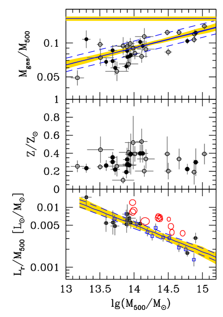
Figure 1: Various quantities are plotted as a function of the total cluster mass within $r_{500}$. Filled circles refer to our sample of 12 clusters from Table 1, with $M_{\rm gas}$ and $M_{500}$ from Vikhlinin et al. (2006) and Sun et al. (2009), metallicity $Z$ from Vikhlinin et al. (2005) and Sun et al. (2012) and $L_{\rm r}$ from Andreon (2012a). All these four parameters are measured homogeneously within consistent radii. Open circles refer to clusters from the same sources, but for which no $L_{\rm r}$ measurements are available. Top panel: the cluster gas fraction with the corresponding best-fit linear relation. The horizontal line is drawn at the level of cosmic baryon fraction = 0.165. Middle Panel: The ICM iron abundance. Bottom Panel: The cluster $L_{\rm r}/M_{500}$ ratio. Open squares refer to clusters from Andreon (2012a) for which ICM mass and metaliicity have not been measured in Vikhlinin et al. (2006) and Sun et al. (2009). These are typically stacks of 5 clusters. The small red ellipses refer to the clusters from Gonzalez et al. (2013) with their axes corresponding to 1$\sigma$ error bars. For the offset affecting the Gonzalez et al. sample see the main text. In the top and bottom panels the best-fit relations to the 12 clusters and their uncertainty range are also shown, with the yellow band representing the 1-$\sigma$ error from the best fit and the blue dashed lines the best fit linear relation $\pm$ the 1-$\sigma$ intrinsic scatter

Based on the very same X-ray data, cluster metallicities have been derived by Sun (2012) and Vikhlinin et al. (2005) via spectral fitting and their results are also reported in Table 1. These metallicities are mass-weighted over the whole ICM, and are typically $\sim 30\%$ lower than the luminosity-weighted ones that come directly from the X-ray spectral fits. Hence, unlike luminosity-weighted ones they are not affected by the central abundance enhancement, which is typically $\sim 5\%$ in mass within $r_{500}$, or $\sim 10\%$ within $r_{2500}$ (e.g. De Grandi et al. 2004). For this reason, we adopt deprojected mass–weighted metal abundance between $0.3<r/r_{500}<0.6$ for clusters in Sun et al. (2009) and in A2092 (the latter from M. Sun, private communication). Two clusters (A1795 and A2029) in our primary sample lack a mass-weighted metallicity measurement from Sun et al. (2009) and Vikhlinin et al. (2005). For A1795 we adopt from Vikhlinin et al. (2006) the mean abundance measured outside the central Fe enhancement region, at $r\approx 0.45r_{500}$ . For A2029 we adopt 0.3 solar for the iron abuncance outside its central cool core (2003 and references therein). The average iron abundance of the ICM of the 12 clusters in Table 1 is therefore $\hbox{$Z^{\rm Fe}_{\rm ICM}$}\simeq 0.3\hbox{$Z^{\odot}_{\rm Fe}$}$. These abundances are in the (1989) scale where $\hbox{$Z^{\odot}_{\rm Fe}$}=0.0018$, and have been updated for the recent change of the Chandra calibration, an upward (abundance) change by a factor 1.12 (Andreon, 2012b). Iron abundance data exist for a much larger sample of clusters than reported on this figure, showing that at least above $\sim 2$ keV the iron abundance is independent of ICM temperature, hence mass (e.g., Andreon 2012b, and references therein). Thus, an abundance $\sim 0.3$ solar appears to be applicable to all massive clusters studied so far.

The $r$-band luminosity, $L_{\rm r}$ within the radiii $r_{500}$ and $r_{200}$ has been derived in Andreon (2012a) using SDSS data by integrating the luminosity function of the red cluster galaxies, adding up the luminosity of the BCG and the galaxy light below the detection threshold (by extrapolating the luminosity function, see Andreon 2010 and Andreon 2012a for details). The $L_{\rm r}$ value of A2029 reported in Table 1 has been recomputed from CFHT MegaCam images, strictly following the same procedure, because SDSS data turned out to be partially corrupted at the sky location of A2029 (S. Andreon, in preparation). Red galaxies are those within 0.1 redward and 0.2 blueward in $g-r$ with respect to the red sequence in the colour–magnitude plot of each individual cluster. The intracluster light is negligible within such large radii (Zibetti et al. 2005; Andreon 2010; Giallongo et al. 2014; Presotto et al. 2014) once one accounts for the light emitted by undetected galaxies, by the outer regions of galaxies and by the BCG, which are all included in the present estimates of $L_{\rm r}$. As for all other quantities, $L_{\rm r}$ is the deprojected value within the sphere of radius $r_{500}$ (or $r_{200}$). For this deprojection the cluster light is assumed to follow a NFW distribution (Navarro, Frenk & White, 1997).

We supplement this sample of relaxed clusters, having both top-quality X-ray data and $L_{\rm r}$ measurements, with other cluster samples with less complete datasets but which help establishing the main trends. These secondary samples include either relaxed cluster missing measurements of the optical luminosity, or clusters with masses derived from the caustic technique without any restiction on their dynamical status. Also for these samples, measurements are performed within consistent radii. Thus, we also consider the clusters in Vikhlinin et al. (2006) and Sun et al. (2009) lacking a measured $L_{\rm r}$ but which are useful to delineate the mass dependency of the gas fraction and metallicity. Besides them, we also consider clusters from Andreon (2010) with high quality $L_{\rm r}$, but lacking high-quality X-ray data. This supplementary sample consists of 54 clusters with dynamical (caustic) masses derived from their estimated escape velocity with a typical $0.15$ dex error (Rines & Diaferio 2006). These clusters are selected independently of their dynamical status, and their masses, unlike those derived from X-ray data, do not assume hydrostatic equilibrium and the relaxed status of the cluster. On the other hand, these measurements make a (weak) assumption about the velocity dispersion anysotropy. The $r$-band luminosity of these clusters have been derived as for the primary sample, except that measurements were performed only within $r_{200}$ (Andreon, 2010). This sample helps to delineate the mass-dependency of $\hbox{$L_{\rm r}$}/M_{500}$, hence of the stellar fraction, confirming the trend derived from the 12 primary clusters.

Finally, we use also the cluster sample from Gonzalez et al. (2013), where core-excised X-ray temperatures were measured and total masses were derived assuming a mass vs X-ray temperature relation. From their deprojected stellar masses we removed the $M/L_{\rm I}$ ratio assumed by the authors (2.65), and we then converted the resulting $I$-band luminosities into $r$-band ones using Maraston (2005) models for a Kroupa IMF, solar metallicity, 11 Gyr old simple stellar population. No iron abundances are available for these clusters.

4 Results

The top panel of Figure 1 shows the gas fraction as a function of the cluster mass for the clusters in Vikhlinin et al. (2006) and Sun et al. (2009); filled circles refers to objects in our primary sample. The corresponding best fit relation is:

$$\hbox{{\rm log}$\,$}\frac{M_{gas,500}}{M_{500}}\simeq(0.15\pm 0.03)(\hbox{{\rm log}$\,$}M_{500}-14.5)-0.97\pm 0.02.$$ (9)

There is a modest increase of the gas fraction with cluster mass, as already pointed out in the literature (Sun et al., 2009; Andreon, 2010; Gonzalez et al., 2013). After accounting for observational errors the intrinsic scatter is also small ($\sim 15$ %), indicating minor cluster to cluster stochasticity in gas fractions (Andreon 2010).

The middle panel of Figure 1 shows the observed iron abundances in the ICM (mass weighted). There is no appreciable trend of iron abundance with cluster mass, i.e., $\hbox{$Z^{\rm Fe}$}\simeq$ constant, apart from a hint for a possible local maximum around $M_{500}=10^{14}\,\hbox{$M_{\odot}$}$, resulting from an apparent maximum in clusters with $kT\simeq 2$ keV which may be spurious (Renzini, 1997). This virtually constant iron abundance is found also among the 130 clusters (mostly with $kT>3$ keV) in Andreon (2012b). For these clusters the iron abundances are still luminosity-weighted and non-core excised.

Finally, the bottom panel of Figure 1 shows the cluster light-to-mass ratio $\hbox{$L_{\rm r}$}/M_{500}$: the cluster $r$-band luminosity is not proportional to the cluster mass, but its growth is much slower, i.e., massive clusters emit less luminosity per unit cluster mass than less massive clusters (Andreon, 2010, 2012a; Gonzalez et al., 2013). As in the rest of the figure, the solid circles in the the bottom panel refer to our primary sample, with data being best fitted by:

$$\hbox{{\rm log}$\,$}\frac{L_{\rm r,500}}{M_{500}}=-(0.45\pm 0.08)({\rm log}M_{500}-14.5)-2.51\pm 0.05,$$ (10)

which is also reported in the bottom panel. This best fit relation provides also an excellent match to other datasets, namely the full sample from Andreon (2010) (the open squares in Figure 1, where all quantities are however measured within $r_{200}$ instead of within $r_{500}$) and the sample from Gonzalez et al. (2013) (red ellipses in Figure 1). Notice that for the former set of clusters the open squares in Figure 1 refer to the stack in groups up to five each, so to reduce the scatter given the larger errors. The offset of the latter set of clusters seen on the bottom panel of Figure 1 compared to the other clusters may be partly due to a differential selection effect. Gonzalez et al. (2013) clusters are indeed drawn from an optically-selected sample and have a very dominant galaxy (BCG) contributing up to 40% to the total luminosity, thus are not selected independenty of the quantity being measured (the cluster optical luminosity). Instead, the other clusters in Figure 1 are selected in X-ray, hence independenty of their optical luminosity. Moreover, part of the offset may well be due to the known systematic differences in mass estimates (Rozo et al., 2014; Applegate et al., 2014; von der Linden et al., 2014), which once more illustrates the need for using homeogeneously derived quantities as much as possible.

All in all, once a vertical/horizontal offset is allowed to account for selection effects the three sets of clusters (75 clusters in total) appear to define a tight $\hbox{$L_{\rm r}$}-M$ relation, with the $\hbox{$L_{\rm r}$}/M$ ratio dropping by a factor $\sim 3$ for cluster masses between $10^{14}$ and $10^{15}\,\hbox{$M_{\odot}$}$.

We recall that for clusters shown as circles in Figure 1 $M_{500}$ was measured from X-ray data assuming hydrostatic equilibrium, whereas for clusters shown as open squares $M_{200}$ was measured with the caustic method and those shown as ellipses came from the $T_{\rm X}-M$ relation. The agreement of the $\hbox{$L_{\rm r}$}/M_{500}$ ratios (proportional to the stellar mass fraction) vs mass relations among these various datasets (apart from the mentioned offset of Gonzalez et al. clusters) suggests that these mass measurements are consistent with each other. Although with larger errors compared to hydrostatic modelling (typically $\sim 0.15$ dex vs $\sim 0.05$ dex) this in particular applies to masses derived with the caustic method.

At variance with these results, Budzynski et al. (2014) find an almost linear $\hbox{$L_{\rm r}$}-M_{500}$ relation, hence a stellar mass fraction almost constant with total cluster mass. When measuring $L_{\rm r}$ in the same way as in Andreon (2010) (i.e., within $r_{200}$) Budzynski et al. (2014) find the same results as Andreon (2010), so they ascribe the discrepancy to the use of caustic masses for $M_{200}$. However, in Budzynski et al. (2014) cluster masses were not measured directly, but estimated from the cluster richness. One possible origin of the discrepancy is the large scatter of the richness–mass relation and the contamination affecting especially the lower mass clusters, leading to overestimate their total mass, hence to underestimate their stellar fraction (Kravtsov, Vikhlinin & Meshscheryakov 2014). In any event, a decreasing trend of the stellar mass to halo mass ratio, similar to that shown in Figure 1, is found in many studies dealing with the efficiency of baryon-to-stars conversion as a function of halo mass (e.g., Leauthaud et al. 2012; Behroozi, Wechsler & Conroy 2013; Kravtsov, Vikhlinin & Meshscheryakov 2014; Birrer et al. 2014).

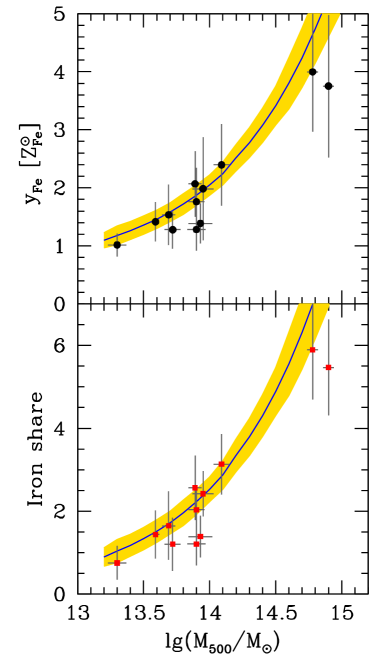
Figure 2: Upper Panel: the apparent iron yield for the 12 clusters in Table 1 as a function of $M_{500}$, using Equation (12). The relation implied together by Equation (9) and Equation (10) is also shown, with the yellow error band corresponding to those shown in Figure 1, and assuming an iron abundance 0.3 solar (the average of the data shown in Figure 1). Lower Panel: the corresponding iron share, i.e., the ratio of iron mass in the cluster ICM over that in galaxies. Notice that these yields are in units where $\hbox{$Z^{\odot}_{\rm Fe}$}=0.00124$.

5 Implications

The striking implication of combining the information in the three panels of Figure 1 is that the total mass of iron in the ICM = $\hbox{$Z^{\rm Fe}_{\rm ICM}$}*M_{gas,500}$ increases with cluster mass while the $\hbox{$L_{\rm r}$}/M_{500}$ ratio (i.e., the stellar mass fraction) decreases. Taking Figure 1 at face value, such a decrease is a factor of $\sim 10$ over 2 dex in $M_{500}$, and yet the iron abundance in the ICM remains the same ($\sim 0.3\times$ solar) in spite of the drop in the mass fraction of the stars which should have produced such mass of iron. In more precise quantitative terms, one can estimate the empirical iron yield as:

$$\hbox{$y_{\rm Fe}$}=\hbox{$Z^{\odot}_{\rm Fe}$}{{\hbox{$M_{\rm stars}$}+1.45(\hbox{$Z^{\rm Fe}_{\rm ICM}$}/\hbox{$Z^{\odot}_{\rm Fe}$})\times M_{\rm gas}}\over\hbox{$M_{\rm stars}$}(0)},$$ (11)

where it is assumed that the average iron abundance in the cluster stars is solar and $\hbox{$M_{\rm stars}$}(0)$ is the mass of gas that went into stars whose present mass is now reduced to $M_{\rm stars}$ by the mass return from stellar mass loss. This equation can be further elaborated into:

$$\hbox{$y_{\rm Fe}$}=\hbox{$Z^{\odot}_{\rm Fe}$}{\hbox{$M_{\rm stars}$}\over\hbox{$M_{\rm stars}$}(0)}\bigl{(}1+1.45{\hbox{$Z^{\rm Fe}_{\rm ICM}$}\over\hbox{$Z^{\odot}_{\rm Fe}$}}\times{M_{\rm gas}\over\hbox{$L_{\rm r}$}}\times{\hbox{$L_{\rm r}$}\over\hbox{$M_{\rm stars}$}}\bigr{)},$$ (12)

where $Z^{\odot}_{\rm Fe}$ in front of these expression is the photospheric iron from Asplund et al. (2009), $\hbox{$Z^{\rm Fe}_{\rm ICM}$}/\hbox{$Z^{\odot}_{\rm Fe}$}$ comes from Table 1 and the factor 1.45 is the ratio of the photospheric solar iron abundance from (1989) over that from Asplund et al. (2009). We then adopt for the residual to initial mass ratio $\hbox{$M_{\rm stars}$}/\hbox{$M_{\rm stars}$}(0)=0.58$ and $\hbox{$M_{\rm stars}$}/\hbox{$L_{\rm r}$}=3.24$, as appropriate for a solar metallicity, 11 Gyr old simple stellar population with “Krupa IMF”, as from the synthetic models of Maraston (2005). These expressions for the yield assume that all clusters have evolved as closed systems as far as metals and stars are concerned, which may not be the case (see below).

Figure 2 shows the resulting empircal yields having fed data in Table 1 into Equation (12). This apparent yield is in the range between $\sim 1$ and 2$\times\hbox{$Z^{\odot}_{\rm Fe}$}$ for clusters with total mass up to $\sim 10^{14}\,\hbox{$M_{\odot}$}$, just as expected from the semiempirical estimates summarized in Equation (6). However, for the two most massive clusters of the sample the iron yield turns out to be $\sim 3$ times solar, with a rising trend with cluster mass which is primarily driven by the decreasing trend in $\hbox{$L_{\rm r}$}/M_{500}$ (hence stellar mass fraction) shown in Figure 1. Much of these trends is due to very low $L_{\rm r}$ luminosity for their total mass of the two most massive clusters and one may argue that these two clusters may be exceptional, or that some of their parameters were erroneously estimated. The fact is, however, that these two clusters follow the general trend shown in Figure 1, hence they do not appear to be exceptional outliers. Indeed, the Gonzalez et al. (2013) and Andreon (2010) clusters nicely fill the gap between the lower mass clusters and the two most massive ones in our primary sample. The same data are shown in Figure 3 as a function of ICM temperature, where the (possibly spurious) bump at $T_{\rm X}\sim 2$ keV is also apparent.

We emphasize that the increasing iron yield with cluster mass is the combined result of a decreasing $\hbox{$L_{\rm r}$}/M_{500}$ and a constant metallicity. For deriving the $\hbox{$L_{\rm r}$}/M_{500}$ trend we use three independent measurements (Gonzalez et al., 2013; Andreon, 2010, 2012a) whereas the constancy of metallicity is well documented in the literature for large cluster samples (e.g. the 130 clusters in Andreon 2012b). Thus, this trend is driven by a large sample of data, not just by the two most massive clusters clusters in our primary sample.

Figures 2 and 3 show also the iron share between the ICM and galaxies, as from Equation (5), once more assuming that the average metallicity of the stars is solar. Again, for clusters up to $\sim 10^{14}\,\hbox{$M_{\odot}$}$ the iron share is between $\sim 1$ and 2, but for the two most massive clusters it appears to be much higher, around $\sim 4$, i.e., there appears to be $\sim 4$ times more iron out of galaxies than within them!

Figure 4 shows in red the baryon fraction of the clusters, i.e., $(\hbox{$M_{\rm stars}$}+M_{\rm gas})/M_{500}$, both for our primary cluster sample (filled circles) and for the sample of Gonzalez et al. (2013) (filled squares). Notice that this bayon fraction lies systematically below the cosmic fraction 0.165 and appears to increase slightly with cluster mass (ignoring the least massive cluster) as generally found (e.g., Andreon 2010; Leauthaud et al. 2012; Gonzalez et al. 2013; Lin et al. 2012; see also the compilation in Planelles et al. 2013). This suggests that baryons are more broadly distributed than the dark matter dominating the cluster potential and a fraction of them may have been lost from (or never incorporated in) clusters, and especially so in groups and the least massive clusters (e.g., Renzini et al. 1993). The same figure also shows in blue the fraction of the baryons which are now in stars, i.e., $\hbox{$M_{\rm stars}$}/(\hbox{$M_{\rm stars}$}+M_{\rm gas})$, for both samples of clusters. A systematic decline of the star fraction with increasing cluster mass is common to both samples. Notice that among clusters with $M_{500}\simeq 10^{14}\,\hbox{$M_{\odot}$}$ this fraction is in the range $\sim 0.2-0.3$, not too different from the value 0.17 adopted in Section 2 and substantially higher than the 0.1 value preferred by Loewenstein (2013). However, the most massive clusters appear to be characterized by much smaller values, down to $\sim 0.06$.

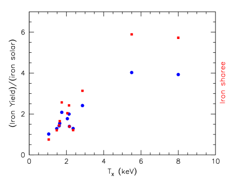
Figure 3: The iron yield (blue circles) and share (red squares) as in Figure 2 but as a function of cluster temperature for the clusters in Table 1

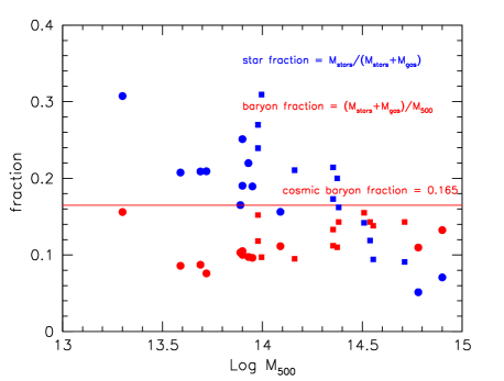
Figure 4: The star fraction (blue) and the baryon fraction (red) of the clusters in our primary cluster sample (filled scircles) and in the sample of Gozalez et al. (2013) (filled squares)

6 (Im)Possible Interpretations: The Conundrum

Clusters up to $\sim 10^{14}\,\hbox{$M_{\odot}$}$ apparently pose no serious challenge. Their empirical iron yield is between $\sim 1$ and $\sim 2$ solar, within the expected range from supernova yields, and their iron share is also between $\sim 1$ and $\sim 2$, as known since a long time. Still, their baryon fraction is appreciably below the cosmic value, indicating that the missing baryons were never incorporated within the halo now hosting the clusters, or were ejected (i.e., beyond $r_{500}$ for this work) from it under the action of some feedback. In the latter case, metals may have been ejected as well, along with the rest of the baryons, hence the above empirical iron yields should be regarded as lower limits.

The problem arises from the more massive clusters, which apparently demand yields well above solar and an iron share dramatically in favor of the ICM. We emphasize again that the problem does not arise uniquely from the two most massive clusters shown in Figure 1 and Figure 2, but instead it does from the apparently well established trends with cluster mass of the gas fraction, the stellar fraction and the metallicity, all illustrated in Figure 1. The comundrum arises from the factor of several drop of the stellar fraction [$\propto\hbox{$L_{\rm r}$}/(\hbox{$M_{\rm stars}$}+M_{\rm gas})$] with increasing cluster mass which would demand a corresponding drop in metallicity, whereas the metallicity appears to be constant among all clusters.

We now list, in casual order, possible solutions of this conundrum.

• In the most massive clusters there are several times more stars out of galaxies than inside them, or, equivalently, the intracluster light exceeds by such factor the luminosity of all the cluster galaxies. Against this possible solution is lack of any evidence for such missing intracluster light (e.g., Zibetti et al. 2005; Andreon 2010; Giallongo et al. 2014).

• The slope of the IMF above $\sim 1\,\hbox{$M_{\odot}$}$ tightly correlates with the present mass of the clusters, i.e., not with the mass of the galaxies as occasionally invoked (e.g., Cappellari et al. 2012). Star-forming clouds at $z{\mathrel{\mathchoice{\lower 2.9pt\vbox{\halign{$\m@th\displaystyle\hfil#\hfil$\cr>\crcr\sim\crcr}}}{\lower 2.9pt\vbox{\halign{$\m@th\textstyle\hfil#\hfil$\cr>\crcr\sim\crcr}}}{\lower 2.9pt\vbox{\halign{$\m@th\scriptstyle\hfil#\hfil$\cr>\crcr\sim\crcr}}}{\lower 2.9pt\vbox{\halign{$\m@th\scriptscriptstyle\hfil#\hfil$\cr>\crcr\sim\crcr}}}}}2$ should know in advance the mass of the clusters in which their products will be hosted ${\mathrel{\mathchoice{\lower 2.9pt\vbox{\halign{$\m@th\displaystyle\hfil#\hfil$\cr>\crcr\sim\crcr}}}{\lower 2.9pt\vbox{\halign{$\m@th\textstyle\hfil#\hfil$\cr>\crcr\sim\crcr}}}{\lower 2.9pt\vbox{\halign{$\m@th\scriptstyle\hfil#\hfil$\cr>\crcr\sim\crcr}}}{\lower 2.9pt\vbox{\halign{$\m@th\scriptscriptstyle\hfil#\hfil$\cr>\crcr\sim\crcr}}}}}10$ Gyrs later. As a kind of last resort, IMF systematic variations have been often invoked to fix problems, and this may be one more example. However, this would demand that galaxies of given mass would have experienced different IMFs in clusters with different mass, hence there should be systematic cluster-to-cluster differences in the galaxy properties for which there is no evidence. For example, cluster early-type galaxies follow closely the same fundamental plane relation, irrespective of the cluster mass (e.g., Renzini 2006 and references therein).

• As a variant to the above option one may think that the special (flat) IMF is a specific property of the BCGs in the most massive clusters, as in some of them massive starburst may be fed from intermitted cooling catastrophies of the ICM, hence representing a different star formation mode (McDonald et al., 2010). However, especially among the most massive clusters, BCGs account for only a small fraction of the total cluster light and stellar mass. Hence, their IMF should be really extreme for them to dominate the metal production of a whole cluster. For example, in the two most massive clusters of our primary sample the BCGs account for only up to $\sim 15\%$ of the total cluster light, hence their metal yield should be ${\mathrel{\mathchoice{\lower 2.9pt\vbox{\halign{$\m@th\displaystyle\hfil#\hfil$\cr>\crcr\sim\crcr}}}{\lower 2.9pt\vbox{\halign{$\m@th\textstyle\hfil#\hfil$\cr>\crcr\sim\crcr}}}{\lower 2.9pt\vbox{\halign{$\m@th\scriptstyle\hfil#\hfil$\cr>\crcr\sim\crcr}}}{\lower 2.9pt\vbox{\halign{$\m@th\scriptscriptstyle\hfil#\hfil$\cr>\crcr\sim\crcr}}}}}20$ times solar for them to account for most of the cluster metals.

• The yield is universal and extremely high ($\sim 4\,\hbox{$Z_{\odot}$}$) but only the most massive clusters have retained nearly all the metals, with most metals having instead been lost by other, less massive clusters. Formally, this might be accompleshed by an IMF substantially flatter than Salpeter above $\sim 1\,\hbox{$M_{\odot}$}$ and/or with a subtantially higher SNIa productivity $k_{\rm Ia}$ than reported in Section 2. This may not contradict other evidences on cluster galaxies, but it remains an ad hoc fix with no independent evidences favoring it.

• The apparent lack of a correlation between ICM metallicity and the stellar fraction may even suggest that the stellar populations of cluster galaxies have little to do with the production of the metals now dispersed in the ICM (e.g., Loewenstein 2001; Bregman, Anderson & Dai 2010; Loewenstein 2013; Morsony et al. 201a). In this view, metals may have been produced by an early stellar generation of very massive and/or Population III stars, leaving virtually no present-day low mass star counterparts. Like the others, also this solution to the conundrum lacks independed observational evidence and would actually require some cosmic conspiracy to ensure that ICM elemental ratios turn out nearly solar, as observed (see Matsushita et al. 2013 and references therein), in spite of a radically different star formation mode compared to the Galactic disk. Moreover, were Population III the solution to the conundrum, this would imply an extremely high clustering of Pop. III star, as such high metal pedestal is found only in the most massive clusters. Extremely low metallicity stars are indeed quite common within the Local Group, hence by comparison with the clusters should have escaped virtually any pollution from Pop. III stars.

• As none of the above solutions is easy to accept, we must retain the option that some of the observations illustrated in Figure 1 may be faulty. The two most critical ones for the generation of the cunundrum are the drop in $\hbox{$L_{\rm r}$}/M_{500}$ coupled to the constancy of metallicity. We have already mentioned that Budzynski et al. (2014) find a constant run of $\hbox{$L_{\rm r}$}/M_{500}$, which automatically avoids the conundrum altogether. But we have noticed that their measure of $M_{500}$ is of lower quality, being obtained from the cluster mass-richness relation instead than from modelling the X-ray surface brightness distribution. The alternative is that the measured metallicity is systemathically overstimated with increasing cluster mass, which appears rather implausible given the quality of the current X-ray data.

In summary, none of these possible solutions of the conundrum appears attractive to us, hence we are left with no solution at all.

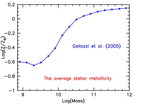
Figure 5: The stellar metallicity vs. stellar mass relation for local galaxies as from Table 2 in Gallazzi et al. (2005)

7 Past Metal Production as a Function of Galaxy Mass

In this section we further explore some consequences of the finding that there is at least as much iron dispersed in the ICM as there is still locked into the cluster stars and galaxies. In particular, having empirically estimated the metal yield ($y$) we aim to estimate the relative contribution of cluster galaxies to the metals now in the ICM, as a function of galaxy mass, thus setting constraints on the amount of metals individual galaxies should have lost.

It is well established that the metallicity of galaxies is an increasing function of their stellar mass, both in the stellar as well as in the gas components, both locally as well as at high redshift. From the SDSS database, Tremonti et al. (2004) and Gallazzi et al. (2005) have derived the stellar mass-metallicity relation for the ISM and for stars of local galaxies, respectively. At higher redshifts the (ISM) mass-metallicity relation shifts to lower metallicities (e.g. Erb et al. 2006), possibly becoming steeper as a function of mass (Zahid et al., 2013).

Figure 5 shows the stellar metallicity of local galaxies as a function of stellar mass, as from Table 2 in Gallazzi et al. (2005). A similar flattening at high masses is also present when considering the ISM metallicity, and Tremonti et al. (2004) interpreted it as the most massive galaxies being able to retain virtually all the metals produced by stars in the course of all previous evolution, whereas lower mass galaxies would have lost in a wind (a major) part of them. However, at high redshifts evidence for galactic winds is ubiquitous for star-forming galaxies of all masses (e.g., Pettini et al. 2000; Newman et al. 2012), with a mass loading factor (= ratio of the mass loss rate to the star formation rate, SFR) of order of unity or higher (Newman et al. 2012; Lilly et al. 2013). Thus, even the most massive galaxies must have lost a substantial fraction of their metals, at least during their early evolution when both their mass and SFR were growing rapidly (Renzini, 2009; Peng et al., 2010). We actually interpret the asymptotic plateau at high masses as a result of galaxies turning passive due to mass quenching of star formation (Peng et al., 2010). Thus, in this section we try to quantify how much metal mass should have been lost even by the most massive galaxies in order to achieve a metal-mass share above unity.

In this context one can also introduce the concept of metal mass loading factor of a galaxy (somehow analog to the mass loading factor mentioned above), defined as the ratio of the metal mass lost to the ICM/IGM to the metal mass still locked into its stars. This quantity is then estimated below, for two values of the assumed metal yield.

Here we first assume that the most massive galaxies have retained all the metals that have been produced by the stars now in them, derive from this the implied metal yield and check what would be the resulting metal share between the ICM and galaxies. We then relax this assumption to derive constraints on the metal loss from galaxies if a metal share of order of unity (or higher) is to be achieved, as demanded by the observations (cf. Section 2 and Section 4). We also assume that the global metal yield $y$ is independednt of the metallicity of the parent stellar population, as indeed indicated by theoretical nucleosynthesis (e.g., Nomoto, Kobayashi & Tominaga 2013) according to which $y$ is a weak function of metallicity. We then proceed to calculate what are the fractions of the overall metal production that is now locked into galaxies and that of the metals which have been ejected, both as a function of galaxy mass.

For the mass function of local galaxies we adopt the multi-Schechter fits from Peng et al. (2010), with

$$\phi(M)=\phi_{\rm B}(M)+\phi_{\rm R}(M),$$ (13)

being the sum the mass function of blue (star-forming) and red (quenched) galaxies, with

$$\phi_{\rm B}(M)=\phi^{*}_{\rm B}\left(M\over M^{*}\right)^{-1.4}e^{-M/M^{*}},$$ (14)

and

$$\phi_{\rm R}(M)=\phi^{*}_{\rm 1R}\left(M\over M^{*}\right)^{-0.4}e^{-M/M^{*}}+\phi^{*}_{\rm 2R}\left(M\over M^{*}\right)^{-1.4}e^{-M/M^{*}},$$ (15)

where from Table 3 in Peng et al. (2010) we have $M^{*}=10^{10.67}\,\hbox{$M_{\odot}$}$, $\phi^{*}_{\rm B}=1.014$, $\phi^{*}_{\rm 1R}=3.247$ and $\phi^{*}_{\rm 2R}=0.214$. Masses denoted with $M$ are here intended to be “stellar masses” of individual galaxies, and we omit the subscript “stars” for simplicity.

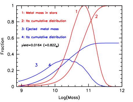
Figure 6: The normalized distributions of the metals inside galaxies and ejected by them, curves 1 and 3, respectively, and the corresponding cumulative distributions, curves 2 and 4. These plots refer to an assumed metal yield $y=0.82\,\hbox{$Z_{\odot}$}$, corresponding to the assumption of most massive galaxies having evolved as a closed box

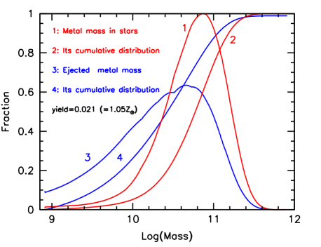
Figure 7: The same as Figure 6 but for $y=1.05\hbox{$Z_{\odot}$}$, which allows metal losses also from the most massive galaxies and ensures an equal share of metals between the ICM and cluster galaxies

By its definition, the total metal yield is given by the ratio of the total metal production over the mass of gas that went into stars:

$$y={M_{\rm Z}^{\rm tot}\over M_{\rm tot}(0)}$$ (16)

where $M_{\rm tot}(0)$, the total mass turned into stars, is given by:

$$M_{\rm tot}(0)={1\over R}\int_{\rm m}^{M}M\,\phi(M)\,dM,$$ (17)

where $R$ is the average residual mass fraction, once taking into account the mass return from dying stars. The value of $R$ depends on the actual star formation history of individual galaxies and its accurate estimate is beyond the scope of this paper. By adopting $R=0.58$ in Section 5 it was assumed that the bulk of stars in cluster galaxies are $\sim 11$ Gyr old, hence all galaxies have the same $R$, and in this section we stick on this assumption. Hence the relation $M(0)=1.72M$ holds when referring to the total stellar mass of individual galaxies as well as to the stellar mass of the galaxy population of a whole cluster.

We now estimate the mass of metals inside galaxies and outside them, as implied by the stellar mass-metallicity relation (MZR) of Gallazzi et al. (2005) and an assumed value for the yield. This MZR does not distinguish between clusters and field, hence we assume that it applies to both environments. However, evidence exists for the increase of the gas-phase metallicity with local overdensity for star-forming satellite galaxies (Peng & Maiolino, 2014). The mass of metals contained in galaxies up to mass $M$ is given by:

$$M_{\rm Z,stars}(M)=\int_{\rm m}^{M}M\,Z(M)\,\phi(M)\,dM,$$ (18)

where $m$ is the minimum mass we are considering, say $\sim 10^{9}\,\hbox{$M_{\odot}$}$. Having assumed that the yield is independent of mass and metallicity, the mass of metals that a galaxy of mass $M$ must have ejected is given by the total production [$\equiv yM(0)$] minus the metals still in the galaxy [$=Z(M)M$] and therefore the mass of metals produced by the same galaxies that are not locked into stars (i.e, that are either in the ISM of individual galaxies or ejected into the intergalactic medium, IGM) is given by:

$$M_{\rm Z,out}(M)=\int_{\rm m}^{M}M\,[y/R-Z(M)]\,\phi(M)\,dM.$$ (19)

The total mass of metals is therefore given by the sum of these two integrals extended to the full mass range ($\sim 10^{12}\,\hbox{$M_{\odot}$}$), i.e., $M_{\rm Z}^{\rm tot}=M_{\rm Z,stars}+M_{\rm Z,out}$. Among local galaxies the gas fraction is a deacreasing function of mass, dropping from $\sim 30\%$ in $10^{10}\,\hbox{$M_{\odot}$}$ galaxies to ${\mathrel{\mathchoice{\lower 2.9pt\vbox{\halign{$\m@th\displaystyle\hfil#\hfil$\cr<\crcr\sim\crcr}}}{\lower 2.9pt\vbox{\halign{$\m@th\textstyle\hfil#\hfil$\cr<\crcr\sim\crcr}}}{\lower 2.9pt\vbox{\halign{$\m@th\scriptstyle\hfil#\hfil$\cr<\crcr\sim\crcr}}}{\lower 2.9pt\vbox{\halign{$\m@th\scriptscriptstyle\hfil#\hfil$\cr<\crcr\sim\crcr}}}}}10\%$ in $10^{11}\,\hbox{$M_{\odot}$}$ galaxies (e.g., Magdis et al. 2012). In the following discussion we neglect the metals contained in the ISM of individual galaxies, as they make a marginal contribution to the global metal budget in the local Universe.

Finally, following its definition, the metal mass loading factor $\lambda_{\rm Z}(M)$ is given by:

$$\lambda_{\rm Z}(M)={y/R-Z(M)\over Z(M)}$$ (20)

We first assume that the most massive galaxies have completely retained all the metals that they have produced. This allows us to estimate the yield as:

$$y={\hbox{$Z_{\rm max}$}M\over M(0)}=0.0164=0.82\hbox{$Z_{\odot}$},$$ (21)

having taken $\hbox{$Z_{\rm max}$}=0.0283$ from Figure 5 and using $\hbox{$Z_{\odot}$}=0.02$. Correspondingly, Figure 6 shows how the mass of metals is distributed among galaxies as given by the integrand of Equation (18) whereas the cumulative distribution $M_{\rm Z,stars}(M)$ is given by the same equation. Moreover, the figure also shows how galaxies in the various mass bins have contributed to the mass of metal now out of stars, as given by the integrand of Equation (19), and the corresponding cumulative distribution. For display purposes, the plots relative to the metals within stars have been normalized to unity, but those relative to metals not locked into stars maintain the proper proportion with respect to the former ones.

Several interesting aspects are self-evident from Figure 6: most of the stellar metals are contained in galaxies with $M\sim M^{*}$ whereas the bulk of ejected metals comes from somewhat lower mass galaxies, as revealed by the peak of curve 3 being shifted to lower masses with thespect to the peak of curve 1 (see also Thomas 1998). Still, most of the action is due to galaxies which today are more massive than $\sim 10^{10}\,\hbox{$M_{\odot}$}$. Perhaps more importantly, under the assumption that the most massive galaxies do not eject any metals, the mass of metals ejected is about half of the mass of metals still locked into galaxies: i.e., $\sim 2/3$ of the metals are in stars and $\sim 1/3$ are dispersed outside galaxies in the IGM (with a minor fraction still in the ISM).

This $\sim 0.5$ share of metals between the IGM/ICM and stars falls somewhat short of the ${\mathrel{\mathchoice{\lower 2.9pt\vbox{\halign{$\m@th\displaystyle\hfil#\hfil$\cr>\crcr\sim\crcr}}}{\lower 2.9pt\vbox{\halign{$\m@th\textstyle\hfil#\hfil$\cr>\crcr\sim\crcr}}}{\lower 2.9pt\vbox{\halign{$\m@th\scriptstyle\hfil#\hfil$\cr>\crcr\sim\crcr}}}{\lower 2.9pt\vbox{\halign{$\m@th\scriptscriptstyle\hfil#\hfil$\cr>\crcr\sim\crcr}}}}}1$ share that is found in clusters of galaxies, as reported in Section 2 and illustrated in Figure 2 and 3. In order to achieve a higher share, more in favor of the IGM/ICM, one has to assume a higher metal yield, i.e., a higher value $y$ in Equation (19). After a few tentatives we find that a value $y=0.021\quad(=1.05\hbox{$Z_{\odot}$})$ gives a nearly fifty-fifty share of metals between IGM/ICM and stars and the corresponding distributions are shown in Figure 7. Having allowed also massive galaxies to lose metals, the mass of the peak metal producers is now higher than in the former case, quite close indeed to $M*$.

It is somehow surprizing (and encouraging) that just with $y=\hbox{$Z_{\odot}$}$ one gets a metal share of unity, not far from the values exhibited by the clusters, at least those of mass up to $\sim 10^{14}\,\hbox{$M_{\odot}$}$. Compared to the previous case, the contibution to metals outside galaxies has nearly doubled at all masses, and more so towards the high mass end. One can conclude that the observed ${\mathrel{\mathchoice{\lower 2.9pt\vbox{\halign{$\m@th\displaystyle\hfil#\hfil$\cr>\crcr\sim\crcr}}}{\lower 2.9pt\vbox{\halign{$\m@th\textstyle\hfil#\hfil$\cr>\crcr\sim\crcr}}}{\lower 2.9pt\vbox{\halign{$\m@th\scriptstyle\hfil#\hfil$\cr>\crcr\sim\crcr}}}{\lower 2.9pt\vbox{\halign{$\m@th\scriptscriptstyle\hfil#\hfil$\cr>\crcr\sim\crcr}}}}}1$ metal share in clusters requires $y{\mathrel{\mathchoice{\lower 2.9pt\vbox{\halign{$\m@th\displaystyle\hfil#\hfil$\cr>\crcr\sim\crcr}}}{\lower 2.9pt\vbox{\halign{$\m@th\textstyle\hfil#\hfil$\cr>\crcr\sim\crcr}}}{\lower 2.9pt\vbox{\halign{$\m@th\scriptstyle\hfil#\hfil$\cr>\crcr\sim\crcr}}}{\lower 2.9pt\vbox{\halign{$\m@th\scriptscriptstyle\hfil#\hfil$\cr>\crcr\sim\crcr}}}}}\hbox{$Z_{\odot}$}$, hence that also the most massive galaxies had to eject a substantial fraction of the metals they have produced. Still, the most massive galaxies do not contribute much to the ICM metals because they are very rare, even if the mass of metals each of them has ejected, i.e., $[1.72y-Z(M)]M$, is actually maximal.

Finally, Figure 8 shows the mass dependence of the metal mass loading factor from Equation (20) for the two values of the yields used above. By construction, in the case of the lower value of $y$ the loading factor vanishes towards high masses. For the higher value of $y$ the loading factor is still $\sim 0.3$ even at the highest masses, i.e., $\sim 1/4$ of the produced metals are ejected and $\sim 3/4$ are retained by such galaxies. Of course, for the higher iron share of the massive clusters a higher yield is required, implying that even the most massive galaxies would have lost the majority of the metals they have produced.

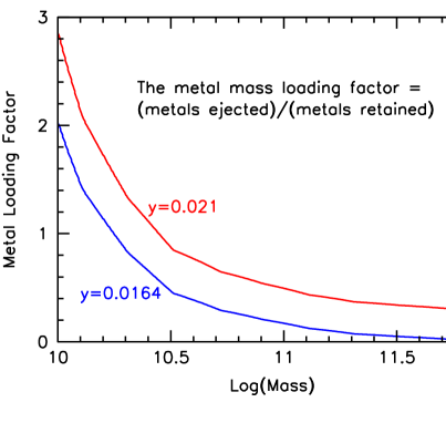
Figure 8: The metal mass loading factor as a function of stellar mass for the two indicated values of the metal yield

8 Conclusions

We have revisited the metal budget of clusters of galaxies using recent cluster data for a sample of clusters for which all four basic parameters are homogeneously measured within consistent radii, namely core-excised, mass-weighted metallicity plus total, stellar and ICM masses. We further use a wider sample of clusters for which one (or two) such parameters are not available, but for which the available data are of high quality. Together, these various samples concur in establishing the trends among the four cluster parameters that we discuss in this paper.

For clusters with mass $M_{500}$ up to $\sim 10^{14}\,\hbox{$M_{\odot}$}$ the total mass of metals is well within the limits expected from standard semi-empirical nucleosynthesis, and a metal yield $y\simeq(1-2)\hbox{$Z_{\odot}$}$. However, when considering more massive clusters a sizable drop of the cluster stellar luminosity per unit cluster mass ($\hbox{$L_{\rm r}$}/M_{500}$) is not accompanied by a drop of the ICM metallicity, as expected if the metal yield is constant. Conversely, the empirical metal yield appears to increase to many times solar for the most massive clusters approaching $M_{500}=10^{15}\,\hbox{$M_{\odot}$}$.

Various possible solutions to this conundrum are discussed, either appealing to missing intracluster light, or systematic cluster-to-cluster differences in the IMF, or of a universal, yet very high metal yield, or even invoking an extinct population of massive stars unrelated to the stellar populations still shining today. Some of such hypothetical solutions appear to be rather astrophysically implausible. Others, although plausible, are not supported by independent evidences, hence remain ad hoc. For these reasons we refrain from favoring any of them. We still cannot exclude the possibility of some systematic bias affecting even the current best measurements of some of the basic cluster parameters, such as their total and ICM mass, the cluster stellar luminosity and the ICM metallicity, but we are not able to identify any obvious bias in the data. We just emphasize that the most serious problem arises from the most massive clusters, with $M_{500}{\mathrel{\mathchoice{\lower 2.9pt\vbox{\halign{$\m@th\displaystyle\hfil#\hfil$\cr>\crcr\sim\crcr}}}{\lower 2.9pt\vbox{\halign{$\m@th\textstyle\hfil#\hfil$\cr>\crcr\sim\crcr}}}{\lower 2.9pt\vbox{\halign{$\m@th\scriptstyle\hfil#\hfil$\cr>\crcr\sim\crcr}}}{\lower 2.9pt\vbox{\halign{$\m@th\scriptscriptstyle\hfil#\hfil$\cr>\crcr\sim\crcr}}}}}5\times 10^{14}\,\hbox{$M_{\odot}$}$, which then would deserve focused observational efforts. Our wish is that this paper could help triggering such efforts.

We include in our study an attempt at estimating the mass of metals that galaxies of given mass must have ejected in the course of their evolution, based on the local stellar mass-metallicity relation and an assumed universal yield (i.e., assuming that the galaxies we see today have produced all the metals). Under these assumptions, it is found that a yield $y=\hbox{$Z_{\odot}$}$ ensures a nearly 50-50 share of metals between the IGM/ICM and stars, close to what observed for typical $M_{500}=10^{14}\,\hbox{$M_{\odot}$}$ clusters. However, for the much higher iron share of the more massive clusters a yield at least twice solar would be required, implying that even the most massive glaxies whould have lost the majority of the metals that have been produced.

References

- (1) Anders, E., & Grevesse, N. 1989, Geochim. Cosmochim. Acta, 53, 197
- Andreon (2010) Andreon, S. 2010, MNRAS, 407, 263
- Andreon (2012a) Andreon, S. 2012a, A&A, 548, A83
- Andreon (2012b) Andreon, S. 2012b, A&A, 546, A6
- Applegate et al. (2014) Applegate, D.E., von der Linden, A., Kelly, P.L., et al. 2014, MNRAS, 439, 48
- Arnaud et al. (1992) Arnaud, M., Rothenflug, R., Boulade, O., Vigroux, L. & Vangioni-Flam, E. 1992, , A&A, 254, 49
- Arnaud et al. (2007) Arnaud, M., Pointecouteau, E. & Pratt, G. W. 2007, A&A, 474, L37
- Asplund et al. (2009) Asplund, M., Grevesse, N., Sauval, A.J. and Scott, P. 2009, ARA&A, 47, 481
- Balestra et al. (2007) Balestra, I., Tozzi, P., Ettori, S., Rosati, P., Borgani, S., Mainieri, V., Norman, C. & Viola, M. 2007, A&A, 462, 429
- Behroozi, Wechsler & Conroy (2013) Behroozi, P.S., Wechsler, R.H. & Conroy, C. 1013, ApJL, 762, L31
- Bender et al. (2014) Bender, A.N., Kennedy, J., Ade, P.A.R., et al. 2014, ApJ, submitted (arXiv:1404.7103)
- Birrer et al. (2014) Birrer, S., Lilly, S., Amara, A., Paranjape, A. & Refregier, A. 2014, ApJ submitted (arXiv:1401.3162)
- Bregman, Anderson & Dai (2010) Bregman, J.N., Anderson, M.E. & Dai, X. 2010, ApJ, 716, L63
- Budzynski et al. (2014) Budzynski, J. M., Koposov, S. E., McCarthy, I. G., & Be lokurov, V. 2014, MNRAS, 437, 1362
- Cappellari et al. (2006) Cappellari, M. et al. 2006, MNRAS, 366, 1126
- Cappellari et al. (2012) Cappellari, M. et al. 2012, Nature, 484, 485
- Chabrier (2003) Chabrier, G. 2003, PASP, 115, 763
- De Grandi et al. (2004) De Grandi, S., Ettori, S., Longhetti, M. & Molendi, S. 2004, A%A, 419, 7
- Erb et al. (2006) Erb, D.K., Shapley, A.E., Pettini, M., Steidel, C.C., Reddy, N.A. & Adelberger, K.L. 2006, ApJ, 644, 813
- Ettori et al. (2009) Ettori, S., Morandi, A., Tozzi, P., Balestra, I., Borgani, S., Rosati, P., Lovisari, L.; & Terenziani, F. 2009, A&A, 501, 61
- Finoguenov et al. (2003) Finoguenov, A. , Burkert, A. & Böhringer, H. 2003, ApJ, 594, 136
- Gallazzi et al. (2005) Gallazzi, A., Charlot, S., Brinchmann, J., White, S.D.M. & Tremonti, C.A. 2005, MNRAS, 362, 41
- Gastaldello et al. (2007) Gastaldello, F. et al. 2007, ApJ, 669, 158
- Giallongo et al. (2014) Giallongo, E. et al. 2014, ApJ, 781, 24
- Giodini et al. (2009) Giodini et al. 2009, ApJ, 703, 982
- Girardi et al. (2000) Girardi, M., Borgani, S., Giuricin, G., Mardirossian, F. & Mezzetti, M. 2000, ApJ, 530, 62
- Gonzalez, Zaritzky & Zabludoff (2007) Gonzalez, A.H., Zaritsky, D. & Zabludoff, A.I. 2007, ApL, 666, 147
- Gonzalez et al. (2013) Gonzalez, A. H., Sivanandam, S., Zabludoff, A. I., & Zaritsky, D. 2013, ApJ, 778, 14
- Greggio & Renzini (2011) Greggio, L. & Renzini, A. 2011, Stellar Populations. A User Guide from Low to High Redshift (Berlin: Whiley-VCH)
- Grego et al. (2001) Grego, L. et al. 2001, ApJ, 552, 2
- Heger & Woosley (2002) Heger, A. & Woosley, S.E. 2002, ApJ, 724, 341
- Howell et al. (2009) Howell, D.A. et al. 2009, ApJ, 691, 661
- Komatsu et al. (2009) Komatsu, E. et al. 2009, ApJS, 180, 330
- Kravtsov, Vikhlinin & Meshscheryakov (2014) Kravtsov, A., Vikhlinin, A. & Meshscheryakov, A. 2014, arXiv:1401.7329
- Kroupa (2001) Kroupa, P. 2001, MNRAS, 322, 231
- Landry et al. (2012) Landry, D., Bonamente, M., Giles, P., Maughan, B., & Joy, M. 2012, MNRAS, submitted (arXiv:1211.4626)
- Leauthaud et al. (2012) Leauthaud, A. et al. 2012, ApJ, 746, 95
- (38) Lewis, A.D., Stocke, J.T. & Buote, D.A. 2002, ApJ, 573, L13
- Lilly et al. (2013) Lilly, S.J.;,Carollo, C.M., Pipino, A., Renzini, A. & Peng, Y. 2013, ApJ, 772, 119
- Lin et al. (2012) Lin, Y., Stanford, S. A., Eisenhardt, P.R.M., Vikhlinin, A., Maughan, B. J. & Kravtsov, A. 2012, ApJ, 745, L3
- Loewenstein (2001) Loewenstein, M. 2013, ApJ, 557, 573
- Loewenstein (2013) Loewenstein, M. 2013, ApJ, 773, 52
- Magdis et al. (2012) Magdis, G.E., Daddi, E., Béthermin, M., Sargent, M., Elbaz, D. et al. 2012, ApJ, 760, 6
- Maraston (2005) Maraston, C. 2005, MNRAS, 362, 799
- Matsushita (2011) Matsushita, K. 2011, A&A, 527, A134
- Matsushita et al. (2013) Matsushita, K., Sakuma, E., Sasaki, T., Sato, K. & Simionescu, A. ApJ, 764, 147
- McDonald et al. (2010) McDonald, M., Bayliss, M., Benson, B.A., Foley, R.J. et al. 2012, Nature, 488, 349
- McGaugh et al. (2010) McGaugh, S.S.; Schombert, J.M.; de Blok, W. J. G.; Zagursky, M.J. 2010, ApJ, 708, L14
- Morsony et al. (201a) Morsony, B.J., Heath, C. & Workman, J.C. 2014, MNRAS, 441, 2134
- Navarro, Frenk & White (1997) Navarro, J. F., Frenk, C. S., & White, S. D. M. 1997, ApJ, 490, 493
- Newman et al. (2012) Newman, S.F. et al. 2012, ApJ, 761, 43
- Nomoto, Kobayashi & Tominaga (2013) Nomoto, K., Kobayashi, C. & Tominaga, N. 2013, ARA&A, 51, 457
- Peng et al. (2010) Peng, Y., Lilly, S.J., Kovač, K., Bolzonella, M., Pozzetti, L., Renzini, A. et al. 2010, ApJ, 721, 193
- Peng & Maiolino (2014) Peng, Y. & Maiolino, R. 2014, MNRAS 438, 262–
- Pettini et al. (2000) Pettini, M., Steidel, C. C., Adelberger, K. L., Dickinson, M., & Giavalisco, M. 2000, ApJ, 528, 96
- Planelles et al. (2013) Planelles, S., Borgani, S., Dolag, K., Ettori, S., Fabjan, D., Murante, G. & Tornatore, L. 2013, MNRAS, 431, 1487
- Pratti et al. (2009) Pratt, G.W., Croston, J.H., Arnaud, M. & Böhringer, H. 2009, A&A, 498, 361
- Presotto et al. (2014) Presotto, V., Girardi, M., Nonino, M. 2014, arXiv/1403.4979
- Renzini et al. (1993) Renzini, A., Ciotti, L., D’Ercole, A. & Pellegrini, S. 1993, ApJ, 419, 52
- Renzini (1997) Renzini, A. 1997, ApJ, 488, 35
- Renzini (2004) Renzini, A. 2004, in Clusters of Galaxies: Probes of Cosmological Structure and Galaxy Evolution, ed. by J.S. Mulchaey, A. Dressler, and A. Oemler (Cambridge Univ. Press), p. 260
- Renzini (2006) Renzini, A. 2006, ARA&A, 44, 141
- Renzini (2009) Renzini, A. 2009, MNRAS, 398, L58
- Rines & Diaferio (2006) Rines, K., & Diaferio, A. 2006, AJ, 132, 1275
- Rozo et al. (2014) Rozo, E., Rykoff, E.S., Bartlett, J.G., & Evrard, A. 2014, MNRAS, 438, 49
- Sanderson et al. (2003) Sanderson, A. J. R., Ponman, T. J., Finoguenov, A., Lloyd-Davies, E. J. & Markevitch, M. 2003, MNRAS, 340, 989
- Sun et al. (2009) Sun, M., Voit, G. M., Donahue, M., et al. 2009, ApJ, 693, 1142
- Sun (2012) Sun, M. 2012, New J. Phys. 14, 045004 (arXiv:1203.4228)
- Thomas (1998) Thomas, D. 1998, arXiv:astro-ph/9811409
- Tremonti et al. (2004) Tremonti, C.A., Heckman, T.M. Kauffmann, G., Brinchmann, J. et al. 2004, ApJ, 613, 898
- Vikhlinin et al. (2005) Vikhlinin, A., Markevitch, M., Murray, S.S. et al. 2005, ApJ, 628, 655
- Vikhlinin et al. (2006) Vikhlinin, A., Kravtsov, A., Forman, W., et al. 2006, ApJ, 640, 691
- Vikhlinin et al. (2009) Vikhlinin, A., Kravtsov, A. V., Burenin, R. A. et al. ApJ, 692, 1060
- von der Linden et al. (2014) von der Linden, A., Mantz, A., Allen, S.W., et al. 2014, MNRAS, submitted (arXiv:1402.2670)
- White et al. (1993) White, S.D.M., Navarro, J.F., Evrard, A.E. & Frenk, C.S. 1993, Nature, 366, 429
- Zahid et al. (2013) Zahid, H. J., Kashino, D., Silverman, J.D., Kewley, L. J., Daddi, E., Renzini, A. et al. 2013, arXiv:1310.4950
- Zampieri (2007) Zampieri, L. 2007, AIPC, 924, 358
- Zibetti et al. (2005) Zibetti, S., White, S. D. M., Schneider, D. P., & Brinkmann, J. 2005, MNRAS, 358, 949