Team Behavior in Interactive Dynamic Influence Diagrams with Applications to Ad Hoc Teams

Abstract

Planning for ad hoc teamwork is challenging because it involves agents collaborating without any prior coordination or communication. The focus is on principled methods for a single agent to cooperate with others. This motivates investigating the ad hoc teamwork problem in the context of individual decision making frameworks. However, individual decision making in multiagent settings faces the task of having to reason about other agents’ actions, which in turn involves reasoning about others. An established approximation that operationalizes this approach is to bound the infinite nesting from below by introducing level 0 models. We show that a consequence of the finitely-nested modeling is that we may not obtain optimal team solutions in cooperative settings. We address this limitation by including models at level 0 whose solutions involve learning. We demonstrate that the learning integrated into planning in the context of interactive dynamic influence diagrams facilitates optimal team behavior, and is applicable to ad hoc teamwork.

, Multiagent systems

1 Introduction

Ad hoc teamwork involves a team of agents coming together to cooperate without any prior coordination or communication protocols [[23]]. The preclusion of prior commonality makes planning in ad hoc settings challenging. For example, well-known cooperative planning frameworks such as the Communicative multiagent team decision problem [[20]] and the decentralized partially observable Markov decision process (DEC-POMDP) [[5]] utilize centralized planning and distribution of local policies among agents, which are assumed to have common initial beliefs. These assumptions make the frameworks unsuitable for ad hoc teamwork.

A focus on how an agent should behave online as an ad hoc teammate informs previous approaches toward planning. This includes an algorithm for online planning in ad hoc teams (OPAT) [[24]] that solves a series of stage games assuming that other agents are optimal with the utility at each stage computed using Monte Carlo tree search. Albrecht and Ramamoorthy [[2]] model the uncertainty about other agents’ types and construct a Harsanyi-Bayesian ad hoc game that is solved online using learning. While these approaches take important steps, they assume that the physical states and actions of others are perfectly observable, which often may not apply.

The focus on individual agents’ behaviors in ad hoc teams motivates that we situate the problem in the context of individual decision-making frameworks. In this regard, recognized frameworks include the interactive POMDP (I-POMDP) [[11]], its graphical counterpart, interactive dynamic influence diagram (I-DID) [[10]], and I-POMDP Lite [[13]]. These frameworks allow considerations of partial observability of the state and uncertainty over the types of other agents with minimal prior assumptions, at the expense of increased computational complexity. Indeed, Albrecht and Ramamoorthy [[2]] note the suitability of these frameworks to the problem of ad hoc teamwork but find the complexity challenging.

While recent advances on model equivalence [[25]] allow frameworks such as I-DIDs to scale, another significant challenge that merits attention is due to the finitely-nested modeling used in these frameworks, which assumes the presence of level 0 models that do not explicitly reason about others [[1], [3], [8], [14]]. A consequence of this approximation is that we may not obtain optimal solutions in cooperative settings. To address this, we augment the I-DID framework by additionally attributing a new type of level 0 model. This type distinguishes itself by utilizing reinforcement learning (RL) either online or in simulation to discover possible collaborative policies that a level 0 agent may execute.

The contributions of this paper are two-fold: First, we show the emergence of true team behavior when the reasoning ability of lower level agents is enhanced via learning. We demonstrate globally optimal teammate solutions when agents are modeled in finitely-nested augmented I-DIDs (Aug. I-DIDs) while traditional I-DIDs fail. Second, we demonstrate the applicability of Aug. I-DIDs to ad hoc settings and show its effectiveness for varying types of teammates. For this, we utilize the ad hoc setting of Wu et al. [[24]], and experiment with multiple well-known cooperative domains. We also perform a baseline comparison of Aug. I-DIDs with an implementation of a generalized version of OPAT that accounts for the partial observability.

2 Background: Interactive DIDs

We sketch I-DIDs below and refer readers to [[25]] for more details.

2.1 Representation

A traditional DID models sequential decision making for a single agent by linking a set of chance, decision and utility nodes over multiple time steps. To consider multiagent interactions, I-DIDs introduce a new type of node called the model node (hexagonal node, $M_{j,l-1}$, in Fig. 1($a$)) that represents how another agent $j$ acts as the subject agent $i$ reasons about its own decisions at level $l$. The model node contains a set of $j$’s candidate models at level $l-1$ ascribed by $i$. A link from the chance node, $S$, to the model node, $M_{j,l-1}$, represents agent $i$’s beliefs over $j$’s models. Specifically, it is a probability distribution in the conditional probability table (CPT) of the chance node, $Mod[M_{j}]$ (in Fig. 1($b$)). An individual model of $j$, $m_{j,l-1}=\langle b_{j,l-1},\hat{\theta}_{j}\rangle$, where $b_{j,l-1}$ is the level $l-1$ belief, and $\hat{\theta}_{j}$ is the agent’s frame encompassing the decision, observation and utility nodes. Each model, $m_{j,l-1}$, could be either a level $l-1$ I-DID or a DID at level 0. Solutions to the model are the predicted behavior of $j$ and are encoded into the chance node, $A_{j}$, through a dashed link, called a policy link. Connecting $A_{j}$ with other nodes in the I-DID structures how agent $j$’s actions influence $i$’s decision-making process.

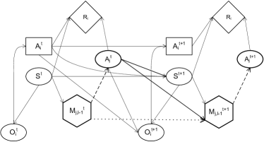
$(a)$

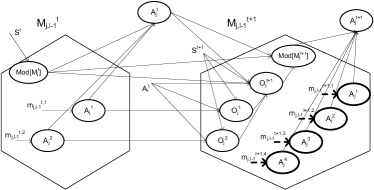
$(b)$

Figure 1: $(a)$ A generic two time-slice level $l$ I-DID for agent $i$. The dotted model update link represents the update of $j$’s models and the distribution over the models over time; $(b)$ Implementation of the model update link using standard dependency links and chance nodes; e.g., two models, $m_{j,l-1}^{t,1}$ and $m_{j,l-1}^{t,2}$, are updated into four models (shown in bold) at time $t+1$.

Expansion of an I-DID involves the update of the model node over time as indicated by the model update link - a dotted link from $M_{j,l-1}^{t}$ to $M_{j,l-1}^{t+1}$ in Fig. 1($a$). As agent $j$ acts and receives observations over time, its models should be updated. For each model $m_{j,l-1}^{t}$ at time $t$, its optimal solutions may include all actions and agent $j$ may receive any of the possible observations. Consequently, the set of the updated models at $t+1$ contains up to $|\mathcal{M}_{j,l-1}^{t}||A_{j}||\Omega_{j}|$ models. Here, $|\mathcal{M}_{j,l-1}^{t}|$ is the number of models at time $t$, and $|A_{j}|$ and $|\Omega_{j}|$ the largest spaces of actions and observations respectively among all the models. The CPT of $Mod[M_{j,l-1}^{t+1}]$ specifies the function, $\tau(b_{j,l-1}^{t},a_{j}^{t},o_{j}^{t+1},b_{j,l-1}^{t+1})$ which is 1 if the belief $b_{j,l-1}^{t}$ in the model $m_{j,l-1}^{t}$ using the action $a_{j}^{t}$ and observation $o_{j}^{t+1}$ updates to $b_{j,l-1}^{t+1}$ in a model $m_{j,l-1}^{t+1}$; otherwise, it is 0. We may implement the model update link using standard dependency links and chance nodes, as shown in Fig. 1($b$), and transform an I-DID into a traditional DID.

2.2 Solution

A level $l$ I-DID of agent $i$ expanded over $T$ time steps is solved in a bottom-up manner. To solve agent $i$’s level $l$ I-DID, all lower level $l-1$ models of agent $j$ must be solved. Solution to a level $l-1$ model, $m_{j,l-1}$, is $j$’s policy that is a mapping from $j$’s observations in $O_{j}$ to the optimal decision in $A_{j}$ given its belief, $b_{j,l-1}$. Subsequently, we may enter $j$’s optimal decisions into the chance node, $A_{j}$, at each time step and expand $j$’s models in $Mod[M_{j,l-1}]$ corresponding to each pair of $j$’s optimal action and observation. We perform this process for each of level $l-1$ models of $j$ at each time step, and obtain the fully expanded level $l$ model. We outline the algorithm for exactly solving I-DIDs in Fig. 2.

The computational complexity of solving I-DIDs is mainly due to the exponential growth of lower $l$-1 $j$’s models over time. Although the space of possible models is very large, not all models need to be considered in the model node. Models that are behaviorally equivalent (BE) [[19]] – whose behavioral predictions for the other agent are identical – could be pruned and a single representative model can be considered. This is because the solution of the subject agent’s I-DID is affected by the behavior of the other agent only; thus we need not distinguish between BE models. Let PruneBehavioralEq ($\mathcal{M}_{j,l-1}$) be the procedure that prunes BE models from $\mathcal{M}_{j,l-1}$ returning the representative models (line 6).

Note that lines 4-5 (in Fig. 2) solve level $l$-1 I-DIDs or DIDs and then supply the policies to level $l$ I-DID. Due to the bounded rationality of level $l$-1 agents, the solutions lead to a suboptimal policy of agent $j$, which certainly compromises agent $i$’s performance in the interactions particularly in a team setting. Also, note that the level 0 models are DIDs that do not involve learning. We will show in the coming sections that solving I-DIDs integrated with RL may generate the expected team behavior among agents $i$ and $j$.

I-DID Exact(level $l\geq 1$ I-DID or level 0 DID, horizon $T$) Expansion Phase 1. For $t$ from 0 to $T-1$ do 2. If $l\geq 1$ then Populate $M_{j,l-1}^{t+1}$ 3. For each $m_{j}^{t}$ in $\mathcal{M}_{j,l-1}^{t}$ do 4. Recursively call algorithm with the $l-1$ I-DID (or DID) that represents $m_{j}^{t}$ and horizon, $T-t$ 5. Map the decision node of the solved I-DID (or DID), $OPT(m_{j}^{t})$, to the corresponding chance node $A_{j}$ 6. $\mathcal{M}_{j,l-1}^{t}$ $\leftarrow$ PruneBehavioralEq($\mathcal{M}_{j,l-1}^{t}$) 7. For each $m_{j}^{t}$ in $\mathcal{M}_{j,l-1}^{t}$ do 8. For each $a_{j}$ in $OPT(m_{j}^{t})$ do 9. For each $o_{j}$ in $O_{j}$ (part of $m_{j}^{t}$) do 10. Update $j$’s belief, $b_{j}^{t+1}\leftarrow SE(b_{j}^{t},a_{j},o_{j})$ 11. $m_{j}^{t+1}$ $\leftarrow$ New I-DID (or DID) with $b_{j}^{t+1}$ 12. $\mathcal{M}_{j,l-1}^{t+1}\overset{\cup}{\leftarrow}\{m_{j}^{t+1}\}$ 13. Add the model node, $M_{j,l-1}^{t+1}$, and the model update link 14. Add the chance, decision, and utility nodes for $t+1$ time slice and the dependency links between them 15. Establish the CPTs for each chance node and utility node Solution Phase 16. If $l\geq 1$ then 17. Represent the model nodes, policy links and the model update links as in Fig. 1 to obtain the DID 18. Apply the standard look-ahead and backup method          to solve the expanded DID

Figure 2: Algorithm for exactly solving a level $l\geq 1$ I-DID or level 0 DID expanded over $T$ time steps.

3 Teamwork in Interactive DIDs

Ad hoc teamwork involves multiple agents working collaboratively in order to optimize the team reward. Each ad hoc agent in the team behaves according to a policy, which maps the agent’s observation history or beliefs to the action(s) it should perform. We begin by showing that the finitely-nested hierarchy in I-DID does not facilitate ad hoc teamwork. However, augmenting the traditional model space with models whose solution is obtained via reinforcement learning provides a way for team behavior to emerge.

3.1 Implausibility of Teamwork

Fig. 3 shows an ad hoc team setting of a two-agent grid meeting problem [[6]]. The agents can detect the presence of a wall on its right ($RW$), left ($LW$) or the absence of it on both sides ($NW$). Given a specific observation, the agent may choose to either move in one of four directions – south ($MS$), north ($MN$), east ($ME$), or west ($MW$), or stay in the same cell ($ST$). Each ad hoc agent, $i$ or $j$, moves in the grid and collects rewards as the number indicated in the occupied cell. If they move to different cells, the agents get their own individual reward. However, if they move to the same cell allowing them to hold an ad hoc meeting, they will be rewarded with twice the sum of their individual rewards. Initial positions of the two agents are shown in color and we focus on their immediate actions.

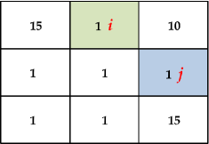
Figure 3: Agents $i$ and $j$ in the grid meeting problem with the numbers being their individual rewards.

If each agent deliberates at its own level, agent $i$ modeled at level 0 will choose to move left while a level 0 agent $j$ chooses to move down. Each agent will obtain a reward of 15 while the whole team gets 30. Agent $i$ modeled at level 1 and modeling $j$ at level 0 thinks that $j$ will move down, and its own best response to predicted $j$’s behavior is to move left. Analogously, a level 1 agent $j$ would choose to move down. A level 2 agent $i$ will predict that a level 1 $j$ moves down as mentioned previously, due to which it decides to move left. Analogously, a level 2 agent $j$ continues to decide to move down. We may apply this reasoning inductively to conclude that level $l$ agents $i$ and $j$ would move left and down, respectively, thereby earning a joint reward of 30. However, the optimal team behavior in this setting is for $i$ to move right and $j$ to move up thereby obtaining a team reward of 40.

Clearly, these finite hierarchical systems preclude the agents’ optimal teamwork due to the bounded reasoning of the lowest level (level 0) agents. The following observation states this more formally:

Observation 1.

There exist cooperative multiagent settings in which rational intentional agents each modeled using the finitely-nested I-DID (or I-POMDP) may not choose the jointly optimal behavior of working together as a team.

Notice that an offline specification of level 0 models in cooperative settings is necessarily incomplete. This is because the true benefit of cooperative actions often hinges on others performing supporting actions, which by themselves may not be highly rewarding to the agent. Thus, despite solving the level 0 models optimally, the agent may not engage in optimal team behavior.

In general, this observation holds for cooperative settings where the self-maximizing level 0 models result in predictions that are not consistent with team behavior. Of course, settings may exist where the level 0 model’s solution coincides with the policy of a teammate thereby leading to joint teamwork. Nevertheless, the significance of this observation is that we cannot rely on finitely-nested I-DIDs to generate optimal teammate policies.

We observe that team behavior is challenging in the context we study above because of the bounded rationality imposed by assuming the existence of a level 0. The boundedness precludes modeling others at the same level as one’s own – as an equal teammate. However, at the same time, this imposition is, $(a)$ motivated by reasons of computability, which allow us to operationalize such a paradigm; and $(b)$ allows us to avoid some self-contradicting, and therefore impossible beliefs, which exist when infinite belief hierarchies are considered [[7]]. Consequently, this work is of significance because it may provide us a way of generating optimal team behavior in finitely-nested frameworks, which so far have been utilized for noncooperative settings, and provides a principled way to solving ad hoc teamwork problems.

3.2 Augmented Level 0 Models that Learn

We present a principled way to induce team behavior by enhancing the reasoning ability of lower-level agents. While it is difficult to a priori discern the benefit of moving up for agent $j$ in Fig. 3, it could be experienced by the agent. Specifically, it may explore moving in different directions including moving up and learn about its benefit from the ensuing, possibly indirect, team reward.

Subsequently, we may expect an agent to learn policies that are consistent with optimal teammate behavior because the corresponding actions provide large reinforcements. For example, given that agent $i$ moves right in Fig. 3, $j$ may choose to move up in its exploration, and thereby receive a large reinforcing reward. This observation motivates formulating level 0 models that utilize RL to generate the predicted policy for the modeled agent. Essentially, we expect that RL with its explorations would compensate for the lack of teamwork caused by bounded reasoning in finitely-nested I-DIDs.

Because the level 0 models generate policies for the modeled agent only, we focus on the modeled agent’s learning problem. However, the rewards in the multiagent setting usually depend on actions of all agents due to which the other agent must be simulated as well. The other agent’s actions are a part of the environment and its presence hidden at level 0, thereby making the problem one of single-agent learning as opposed to one of multi-agent learning.

We augment the level 0 model space, denoted as $\mathcal{M}^{\prime}_{j,0}$, by additionally attributing a new type of level 0 model to the other agent $j$: $m^{\prime}_{j,0}=\langle b_{j,0},\hat{\theta}^{\prime}_{j}\rangle$, where $b_{j,0}$ is $j$’s belief and $\hat{\theta}^{\prime}_{j,0}$ is the frame of the learning model. The frame, $\hat{\theta}^{\prime}_{j,0}$, consists of the learning rate, $\alpha$; a seed policy, $\pi^{\prime}_{j}$, of planning horizon, $T$, which includes a fair amount of exploration; and the chance and utility nodes of the DID along with a candidate policy of agent $i$, which could be an arbitrary policy from $i$’s policy space, $\Pi_{i}$, as agent $i$’s actual behavior is not known. This permits a proper simulation of the environment.

This type of model, $m^{\prime}_{j,0}$, differs from a traditional DID based level 0 model in the aspect that $m^{\prime}_{j,0}$ does not describe the offline planning process of how agent $j$ optimizes its decisions, but allows $j$ to learn an optimal policy, $\pi_{j}$, with the learning rate, either online or in a simulated setting. Different models of agent $j$ differ not only in their learning rates and seed policies, but also in the $i$’s candidate policy that is used. In principle, while the learning rate and seed policies may be held fixed, $j$’s model space could be as large as $i$’s policy space. Consequently, our augmented model space becomes extremely large.

3.3 Model-Free Learning: Generalized MCESP

Learning has been applied to solve decision-making problems in both single- and multi-agent settings. Both model based [[9]] and model free [[15], [18]] learning approaches exist for solving POMDPs. In the multiagent context, Banerjee et al. [[4]] utilized a semi-model based distributed RL for finite horizon DEC-POMDPs. Recently, Ng et al. [[16]] incorporated model learning in the context of I-POMDPs where the subject agent learns the transition and observation probabilities by augmenting the interactive states with frequency counts.

Because the setting in which the learning takes place is partially observable, RL approaches that compute a table of values for state-action pairs do not apply. We adapt Perkin’s Monte Carlo Exploring Starts for POMDPs (MCESP) [[18]], which has been shown to learn good policies in fewer iterations while making no prior assumptions about the agent’s models in order to achieve convergence. MCESP maintains a $Q$ table indexed by observation, $o_{j}$, and action, $a_{j}$, that gives the value of following a policy, $\pi_{j}$, except when observation, $o_{j}$, is obtained at which point action, $a_{j}$, is performed. An agent’s policy in MCESP maps a single observation to actions over $T$ time horizons. We generalize MCESP so that observation histories of length up to $T$, denoted as $\vec{o}$, are mapped to actions. A table entry, $Q_{\vec{o},a}^{\pi_{j}}$, is updated over every simulated trajectory of agent $j$, $\tau$ $=$ $\{$ $*$, $a_{j}^{0}$, $r_{j}^{0}$, $o_{j}^{1}$, $a_{j}^{1}$, $r_{j}^{1}$, $\cdots$, $o_{j}^{T-1}$, $a_{j}^{T-1}$, $r_{j}^{T-1}$, $o_{j}^{T}$ $\}$, where $r_{j}$ is the team reward received. Specifically, the $Q_{\vec{o},a}^{\pi_{j}}$ value is updated as:

$$Q_{\vec{o},a}^{\pi_{j}}\leftarrow(1-\alpha)Q_{\vec{o},a}^{\pi_{j}}+\alpha R_{post-\vec{o}}(\tau)$$ (1)

where $\alpha$ is the learning rate and $R_{post-\vec{o}}(\tau)$ is the sum of rewards of a portion of the observation-action sequence, $\tau$, following the first occurrence of $\vec{o}$ in $\tau$, say at $t^{\prime}$: $R_{post-\vec{o}}(\tau)$=$\sum_{t=t^{\prime}}^{T-1}\gamma^{t}r_{t}$, where $\gamma\in[0,1)$ is the discount factor. Alternate policies are considered by perturbing the action for randomly selected observation histories.

Level 0 agent $j$ learns its policy while agent $i$’s actions are hidden in the environment. In other words, agent $j$ needs to reason with unknown behavior of $i$ while it learns level 0 policy using the generalized MCESP algorithm. Agent $j$ considers the entire policy space of agent $i$, $\Pi_{i}$, and a fixed policy of $i$, $\pi_{i}$($\in\Pi_{i}$), results in one learned $j$’s policy, $\pi_{j}$.

We show the algorithm for solving level 0 models using the generalized MCESP in Fig. 4. The algorithm takes as input agent $j$’s model whose solution is needed and the policy of $i$, which becomes a part of the environment. We repeatedly obtain a trajectory, $\tau$, of length $T$ either by running the agent online or simulating the environment by sampling the states, actions and observations from the appropriate CPTs (lines 5-10). The trajectory is used in evaluating the value of the current policy, $\pi_{j}$, of agent $j$ (line 11). Initially, we utilize the seed policy contained in agent $j$’s model. If another action, $a^{\prime}$, for the observation sequence, $\vec{o}$, is optimal, we update $\pi_{j}$ to conditionally use this action, otherwise the policy remains unchanged (lines 12-13). This is followed by generating a perturbed policy in the neighborhood of the previous one (line 14), and the evaluation cycle is repeated. If the perturbation is discarded several times, we may terminate the iterations and return the current policy.

RL for Level 0 Model ($j$’s model, $m^{\prime}_{j,0}$, $i$’s policy, $\pi_{i}$, $T$) 1. Sample the initial state $s$ from $b_{j,0}$ in $j$’s model 2. Set current policy of $j$ denoted as $\pi_{j}$ using the seed         policy in $j$’s model 3. Set $\tau\leftarrow\{*\}$ (empty observation) 4. Rep eat 5. For $t$ = 0 to $T-1$ do 6. Obtain $i$’s action from $\pi_{i}$ and $j$’s action, $a_{j}^{t}$, from current policy of $j$ using observation history 7. Obtain the next state, $s^{\prime}$, either by performing the actions or sampling 8. Obtain team reward, $r_{j}^{t}$, using state and joint actions 9. Obtain $j$’s observation, $o_{j}^{t+1}$, using next state and joint actions 10. Generate trajectory, $\tau\leftarrow\tau\cup\{a_{j}^{t},r_{j}^{t},o_{j}^{t+1}\}$ 11. Update $Q_{\vec{o},a}^{\pi_{j}}$ according to Eq. 1 12. If $\underset{a^{\prime}}{max}$ $Q_{\vec{o},a^{\prime}}^{\pi_{j}}$ $>$ $Q_{\vec{o},a}^{\pi_{j}}$ 13. $\pi_{j}(\vec{o})\leftarrow a^{\prime}$ 14. Perturb an action, $a$, in $\pi_{j}$ for some $\vec{o}$ 15. Until termination condition is met 16. Return $\pi_{j}$ and $Q^{\pi_{j}}_{\vec{o},a}$

Figure 4: Algorithm for learning agent $j$’s policies when modeled at level 0.

Level 0 agent $j$ learns its policy while agent $i$’s actions are a part of the environment. As we mentioned previously, agent $j$’s level 0 model space is inclusive of the $i$’s policy space, $\Pi_{i}$. As the space of $i$’s policy becomes large particularly for a large planning horizon, it is intractable for $j$ to learn a policy for all $i$’s policies. In addition, considering that few of $i$’s policies are actually collaborative, we formulate a principled way to reduce the full space to those policies of $i$, denoted as $\hat{\Pi}_{i}$, that could be collaborative.

We begin by picking a random initial policy of $i$ and using it in the frame of a new model of $j$. We apply generalized MCESP to this frame to obtain a candidate agent $j$’s policy, $\pi_{j}^{1}$. Next, both the initial policy of $j$ used by MCESP and $i$’s policy is set to $\pi_{j}^{1}$. MCESP then checks for the neighbors of $\pi_{j}^{1}$, which would improve on the joint utility of ($\pi_{j}^{1}$,$\pi_{i}$ $=$ $\pi_{j}^{1}$). If successful, an improved neighboring policy, say $\pi_{j}^{2}$, is returned. This ensures that the joint utility of ($\pi_{j}^{2}$,$\pi_{j}^{1}$) is greater than ($\pi_{j}^{1}$,$\pi_{j}^{1}$). We continue these iterations setting $\pi_{i}$ as $\pi_{j}^{2}$ and using $\pi_{j}^{2}$ as the seed policy. MCESP may not improve on $\pi_{j}^{1}$ if $\pi_{j}^{1}$ is the (local) best response to $\pi_{i}=\pi_{j}^{1}$. Otherwise, both $\pi_{j}^{1}$ and $\pi_{j}^{2}$ are added to the set of candidate predictions of level 0 behavior of $j$. The process is restarted with a different random policy of agent $i$. We demonstrate this method on the 3$\times$3 Grid domain in Fig. 5.

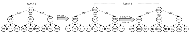
$(a)$ $\pi_{i}$= Random initial policy                   $(b)$ $\pi_{j}$=RL for Level 0 Model ($m^{\prime}_{j,0}$, $\pi_{i}$)   $(c)$ $\pi^{\prime}_{j}$=RL for Level 0 Model ($m^{\prime}_{j,0}$, $\pi_{j})$

Figure 5: We illustrate the principled way to generate collaborative policies for lower level agent $j$ in the 3x3 Grid domain. We start with $(a)$ a random initial policy of agent $i$ in the frame of agent $j$’s model; $(b)$ execute MCESP to generate a collaborative policy for agent $j$; and $(c)$ check whether the neighboring policy of $j$, $\pi_{j}^{\prime}$, has a better joint utility.

3.4 Augmented I-DID Solutions

Solving augmented I-DIDs is similar to solving the traditional I-DIDs except that the candidate models of the agent at level 0 may be learning models. We show the revised algorithm in Fig. 6. When the level 0 model is a learning model, the algorithm invokes the method Level 0 RL shown in Fig. 4. Otherwise, it follows the same procedure as shown in Fig. 2 to recursively solve the lower level models.

While we consider a reduced space of agent $i$’s policies in a principled way, and therefore agent $j$’s learning models, we may further reduce agent $j$’s policy space by keeping top-$K$ policies of $j$, $K$ $>$ 0, in terms of their expected utilities (line 11 in Fig. 4). Observe that across models that differ in $i$’s policy and with the same initial belief, the team behavior(s) is guaranteed to generate the largest utility in a cooperative problem. This motivates focusing on models with higher utilities. Hence, the filtering of $j$’s policy space may not compromise the quality of I-DID solutions at level 1. However, because MCESP may converge to a local optima, the resulting top-$K$ policies are not guaranteed to include $j$’s optimal collaborative policies in theory, although as our experiments demonstrate, we often obtain the optimal team behavior. As the number of optimal policies is unknown, we normally use a sufficiently large $K$ value.

Augmented I-DID (level $l\geq 1$ I-DID or level 0 DID, $T$) Expansion Phase 1. For $~{}t$ from 0 to $T-1$ do 2. If $l\geq 1$ then Populate $M_{j,l-1}^{t+1}$ 3. For  each $m_{j}^{t}$ in $\mathcal{M}_{j,l-1}^{t}$ do 4. If $l>1$ then 5. Recursively call algorithm with the $l-1$ I-DID that represents $m_{j}^{t}$ and the horizon, $T-t$ 6. else 7. If the level 0 model is a learning model then 8. Solve using Level 0 RL in Fig. 4 with horizon, $T-t$ 9. else 10. Recursively call algorithm with level 0 DID and the horizon, $T-t$ 11. Select top-$K$ $j^{\prime}$s policies based on expected utility values given the same belief 12. The remaining steps of the expansion phase are the same           as in Fig. 2. Solution Phase 13. This is similar to the solution phase in Fig. 2.

Figure 6: Algorithm for solving a level $l\geq 1$ I-DID or level 0 DID expanded over $T$ time steps with $M^{\prime}_{j,0}$ containing level 0 models that learn.

Agent $j$’s policy space will be additionally reduced because behaviorally equivalent models – learning and other models with identical solutions – will be clustered [[25]]. In summary, we take several steps to limit the impact of the increase in $j$’s model space. Using a subset of $i$’s policies preempts solving all $j$’s models at level 0 while the top-$K$ technique removes possibly non-collaborative policies.

4 Experimental Results

Our experiments show that I-DIDs augmented with level 0 models that learn facilitate team behavior, which was previously implausible. In addition, we show the applicability of Aug. I-DIDs to ad hoc teamwork in a setting similar to the one used by Wu et al. (). We empirically evaluate the performance in three well-known cooperative domains involving two agents, $i$ and $j$: $3\times 3$ grid meeting (Grid) Bernstein05:Bounded , box-pushing (BP) Seuken07:BoxPush , and multi-access broadcast channel (MABC) Hansen04:MABC . In the BP domain, each agent intends to push either a small or large box into the goal region. The agents’ rewards are maximum when both of them cooperatively push the large box into the goal. In the MABC problem, nodes need to broadcast messages to each other over a channel. Only one node may broadcast at a time, otherwise a collision occurs. The nodes attempt to maximize the throughput of the channel.

Table 1: Domain Dimension and Experimental Settings

Domain	T	$|\mathcal{M}_{j}^{0}|$	$|\hat{\Pi}_{i}|$	Dimension
Grid	3	100	32	$|S_{j}|$=9, $|S_{i}|$=81, $|\Omega|$=3, $|A|$=5
	4	200	100
BP	3	100	32	$|S|$=50, $|\Omega|$=5, $|A|$=4
MABC	3	100	32	$|S_{j}|$=2, $|S_{i}|$=4, $|\Omega|$=2, $|A|$=2
	4	100	64
	5	200	64

We summarize the domain properties and parameter settings of the Aug. I-DID in Table 1. Note that $|\mathcal{M}_{j}^{0}|$ is the number of initial models of agent $j$ at level 0 and $\hat{\Pi}_{i}$ is the subset of $i$’s policies generated using the approach mentioned earlier, allowing us to reduce the full space of $j$’s policies to those that are possibly collaborative.

4.1 Teamwork in Finitely-Nested I-DIDs

Experimental Settings. We implemented the algorithm augmented I-DID as shown in Fig. 6 including an implementation of the generalized MCESP for performing level 0 RL.

We demonstrate the performance of the augmented framework toward generating team behavior. We compare the expected utility of agent $i$’s policies with the values of the optimal team policies obtained using an exact algorithm, GMAA*-ICE, for Dec-POMDP formulations of the same problem domains Spaan08:Multiagent . We also compare with the values obtained by traditional I-DIDs. All I-DIDs are solved using the exact discriminative model update (DMU) method Zeng12:Exploiting . For both traditional and Aug. I-DIDs, we utilized $|\mathcal{M}_{j}^{0}|$ models at level 0 that differ in the initial beliefs or in the frame. We adopt two model weighting schemes: ($a$) Uniform: all policies are uniformly weighted; ($b$) Diverse: let policies with larger expected utility be assigned proportionally larger weights. Note that we maintain the top $K$ by expected utility (out of $|\mathcal{M}_{j}^{0}|$) learning and non-learning models only while solving Aug. I-DIDs. Though the model space is significantly enlarged by the learning policies, Aug. I-DIDs become tractable when both top-$K$ and equivalence techniques are applied.

Table 2: Performance comparison between the trad. I-DID, aug. I-DID, and GMAA*-ICE in terms of the expected utility

	Aug. I-DID			Trad I-DID
Domain	K	Uniform	Diverse	Uniform
Grid	32	41.875	41.93
(T=3)	16	40.95	41.93	25.70
	8	40.95	41.93
	Dec-POMDP(GMAA*-ICE): 43.86
Grid	100	37.15	53.26
(T=4)	64	35.33	53.26	21.55
	32	35.33	53.26
	Dec-POMDP(GMAA*-ICE): 58.75
BP	32	73.45	76.51
(T=3)	16	73.45	76.51	4.75
	8	71.36	76.51
	Dec-POMDP(GMAA*-ICE): 85.18
MABC	32	2.12	2.30
(T=3)	16	2.12	2.30	1.79
	8	2.12	2.30
	Dec-POMDP(GMAA*-ICE): 2.99
MABC	64	3.13	3.17
(T=4)	32	3.13	3.17	2.80
	16	3.13	3.17
	Dec-POMDP(GMAA*-ICE): 3.89
MABC	64	4.08	4.16
(T=5)	32	3.99	4.16	3.29
	16	3.99	4.16
	Dec-POMDP(GMAA*-ICE): 4.79

Performance Evaluation. In Table 2, we observe that the Aug. I-DID significantly outperforms the traditional I-DID where level 0 agent $j$ does not learn. Aug. I-DID’s solutions approach the globally optimal team behavior as generated by GMAA*-ICE. In cooperative games, the globally optimal solution is the pareto optimal Nash equilibrium. We observe that the larger weights on the learned policies lead to better quality $i$’s policies. This restates the importance of the augmented level 0 $j$’s models that learn. The small gap from the optimal DEC-POMDP value is due to the uncertainty over different models of $j$. Note that DEC-POMDPs are informed about the initial belief setting (and do not face the issue of bounded rationality) whereas, I-DIDs are not and they consider the entire candidate model space of $j$. Furthermore, the Aug. I-DID generates the optimal team behavior identical to that provided by GMAA*-ICE when $i$’s belief places probability 1 on the true model of $j$, as is the case for Dec-POMDPs. Increasing $K$ does not have a significant impact on the performance as $K$ is large enough to cover a large fraction of collaborative policies of agent $j$ including the optimal teammate.

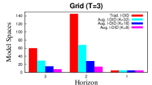
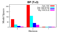
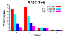
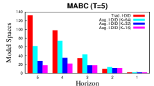
Figure 7: Top-$K$ method reduces the added solution complexity of the augmented I-DID. The complexity is dominated by the model space (number of models) in each time step.

In Fig. 7, we illustrate the reduction of model space that occurs due to smaller values of $K$, which facilitates efficiency in the solution of the Aug. I-DID. Though the augmented level 0 model space is much larger than that of its traditional counterparts, the growth in the number of models is limited due to the top-$K$ heuristic.

4.2 Applications to Ad Hoc Teams

Experimental Settings. We test the performance of the augmented I-DIDs in ad hoc applications involving different teammate types particularly when the teammates’ policies are not effective in advancing the joint goal (i.e. ad hoc) and compare it with a well-known ad hoc planner, OPAT. Teammate types include: ($a$) Random - when the teammate plays according to a randomly generated action sequence for the entire length of the run. Some predefined random seeds are used to guarantee that each test has the same action sequences. ($b$) Predefined - when the teammate plays according to some predefined patterns which are sequences of random actions with some fixed repeated lengths that are randomly chosen at the beginning of each run. For example, if the action pattern is“1324” and the repetition value is 2, the resulting action sequence will be “11332244”. ($c$) Optimal - when the teammate plays rationally and adaptively. OPAT uses an optimal teammate policy for simulations, which is computed offline with the help of a generative model by value iteration. Note that OPAT in its original form assumes perfect observability of the state and joint actions. For comparison, we generalized OPAT to partially observable settings by considering observation sequences.

Additionally, in order to speed up the generation of RL models at level 0, we implemented an approximate version of our generalized MCESP called the Sample Average Approximation (MCESP-SAA) that estimates action values by taking a fixed number of sample trajectories and then comparing the sample averages Perk02:RLPOMDP . We used a sample size of $n$=25 trajectories to compute the approximate value of the policy that generated them, for MCESP-SAA. We set $\alpha$=0.9, and terminate the RL (line 15 in Fig. 4) if no policy changes are recommended after taking $n$ samples of the value of each observation sequence-action pair Perk02:RLPOMDP . We also tested with some domain-specific seed policies to investigate speedup in the convergence of MCESP.

Simulations were run for 20 steps and the average of the cumulative rewards over 10 trials are reported for similar teammate settings for the 3 problems. We show that the augmented I-DID solution significantly outperforms OPAT solutions in all problem domains for random and predefined teammates while performing comparably for optimal ones.

Table 3: Baseline Comparison with OPAT with different types of teammates. Each datapoint is the average of 10 runs.

Ad Hoc Teammate	OPAT	Aug. IDID
Grid T=20, look-ahead=3
Random	12.25 $\pm$ 1.26	14.2 $\pm$ 0.84
Predefined	11.7 $\pm$ 1.63	16.85 $\pm$ 1.35
Optimal	28.35 $\pm$ 2.4	27.96 $\pm$ 1.92
BP T=20, look-ahead=3
Random	29.26 $\pm$ 2.17	36.15 $\pm$ 1.95
Predefined	41.1 $\pm$ 1.55	54.43 $\pm$ 3.38
Optimal	52.11 $\pm$ 0.48	59.2 $\pm$ 1.55
MABC T=20, look-ahead=3
Random	9.68 $\pm$ 1.37	12.13 $\pm$ 1.08
Predefined	12.8 $\pm$ 0.65	13.22 $\pm$ 0.21
Optimal	16.64 $\pm$ 0.28	15.97 $\pm$ 1.31

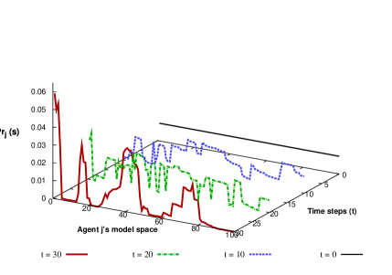
Figure 8: MABC belief updates over 30 steps showing the beliefs converging to fewer models (largest belief is that of agent $j$’s true model).

Performance Evaluation. Table 3 shows that I-DIDs significantly outperform OPAT especially when the other agents are random or predefined types in all three problem domains (Student’s t-test, $p$-value $\leq$ 0.001 for both) except when the teammate is of type predefined in the MABC problem where the improvement over OPAT was not significant at the 0.05 level ($p$-value = 0.0676). Aug. I-DID’s better performance is in part due to the sophisticated belief update that gradually increases the probability on the true model if it is present in agent $j$’s model space as shown in Fig. 8 for MABC. As expected, both OPAT and Aug. I-DID based ad hoc agent perform better when the other agent in the team is optimal in comparison to random or predefined type. Aug. I-DIDs perform significantly better than OPAT when faced with optimal teammates for the BP domain, while the results for the other domains are similar.

In summary, the Aug. I-DID maintains a probability distribution over different types of teammates and updates both the distribution and types over time, which differs from OPAT’s focus on a single optimal behavior of teammates during planning. Consequently, Aug. I-DIDs allow better adaptivity as examined above. Further experiments on the robustness of Aug. I-DIDs in dynamic ad hoc settings showed that agent $i$ obtained significantly better average rewards compared to OPAT ($p$-value = 0.042) for the setting where the other agent is of type predefined and after 15 steps is substituted by an optimal type for the remaining 15 steps in the MABC domain.

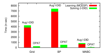
Figure 9: Timing results for augmented I-DID simulations and OPAT with an optimal teammate.

In Fig. 9, we show the online run times for the Aug. I-DID and generalized OPAT approaches on the three problem domains. Expectedly, OPAT takes significantly less time because it approximates the problem by solving a series of stage games modeling the other agent using a single type. In the case of Aug. I-DIDs, we observe that generating and solving the added learning models consume the major portion of the total time. We show the learning overhead for Grid, BP, and the MABC domains in red in the figure. To reduce this overhead and speed up Aug. I-DIDs, an avenue for future work is to try other RL methods in place of MCESP.

4.3 Scalability Results

Although we recognize that the learning component (MCESP) is the bottleneck to scaling augmented I-DIDs for larger problems, we were successful in obtaining the optimal teammate policies using augmented I-DIDs (same as those computed by GMAA*-ICE) in the $4\times 4$ grid, BP for T=4, and MABC for T=5. For these larger problems, we also noticed a significant improvement in the values obtained by augmented I-DIDs over their traditional counterparts as shown in Table 2. In the larger $4\times 4$ grid domain for $T$=3, the optimal team value of 29.6 is achieved by the augmented I-DID compared to 19.82 obtained by solving the traditional I-DID. A better substitute for MCESP and other approximation techniques, will allow us to further scale-up augmented I-DIDs.

5 Discussion and Conclusion

Self-interested individual decision makers face hierarchical (or nested) belief systems in their multiagent planning problems. In this paper, we explicate one negative consequence of bounded rationality: the agent may not behave as an optimal teammate. In the I-DID framework that models individual decision makers who recursively model other agents, we show that reinforcement learning integrated with the planning allows the models to produce sophisticated policies. For the first time, we see the principled and comprehensive emergence of team behavior in I-DID solutions facilitating I-DIDs’ application to ad hoc team settings for which they are just naturally well-suited for. We show that integrating learning in the context of I-DIDs helps us provide a solution to a few fundamental challenges in ad hoc teamwork – building a single autonomous agent that can plan individually in partially observable environments by adapting to different kinds of teammates while making no assumptions about its teammates’ behavior or beliefs and seeking to converge to their true types. Augmented I-DIDs compare well with a standard baseline algorithm, OPAT.

While individual decision-making frameworks such as I-POMDPs and I-DIDs are thought to be well suited for non-cooperative domains, we show that they may be applied to cooperative domains as well. Integrating learning while planning provides a middle ground (or a bridge) between multiagent planning frameworks such as Dec-POMDPs and joint learning for cooperative domains Panait05:CM . Additionally, augmented I-DIDs differentiate themselves from other centralized cooperative frameworks by focusing on the behavior of an individual agent in a multiagent setting. While we recognize that the introduction of learning-based models adds a significant challenge to scaling I-DIDs for larger problems, we successfully obtained optimal teammate policies using Aug. I-DIDs in the $4\times 4$ Grid and BP using a combination of intuitive pruning techniques. By allowing models formalized as I-DIDs or DIDs to vary in the beliefs and frames, we considered an exhaustive and general space of models during planning. The convergence of RL is not predicated on any prior assumptions about other’s models. Immediate lines of future work involve improving the scalability of the framework, particularly its learning component, by utilizing larger problems.

References

- [1] B. Adam and E. Dekel. Hierarchies of beliefs and common knowledge. International Journal of Game Theory, 1993.
- [2] S. Albrecht and S. Ramamoorthy. A game-theoretic model and best-response learning method for ad hoc coordination in multiagent systems (extended abstract). In AAMAS, pages 1155–1156, 2013.
- [3] R. J. Aumann. Interactive epistemology II: Probability. International Journal of Game Theory, 28:301–314, 1999.
- [4] B. Banerjee, J. Lyle, L. Kraemer, and R. Yellamraju. Solving finite horizon decentralized pomdps by distributed reinforcement learning. In AAMAS Workshop on MSDM, pages 9–16, 2012.
- [5] D. S. Bernstein, R. Givan, N. Immerman, and S. Zilberstein. The complexity of decentralized control of Markov decision processes. Mathematics of Operations Research, 27(4):819–840, 2002.
- [6] D. S. Bernstein, E. A. Hansen, and S. Zilberstein. Bounded policy iteration for decentralized pomdps. In IJCAI, 2005.
- [7] K. Binmore. Essays on Foundations of Game Theory. Pittman, 1982.
- [8] C. F. Camerer, T.-H. Ho, and J.-K. Chong. A cognitive hierarchy model of games. The Quarterly Journal of Economics, 119(3):861–898, 2004.
- [9] L. Chrisman. Reinforcement learning with perceptual aliasing: the perceptual distinctions approach. In AAAI, pages 183–188, 1992.
- [10] P. Doshi, Y. Zeng, and Q. Chen. Graphical models for interactive pomdps: Representations and solutions. JAAMAS, 18(3):376–416, 2009.
- [11] P. Gmytrasiewicz and P. Doshi. A framework for sequential planning in multiagent settings. JAIR, 24:49–79, 2005.
- [12] E. A. Hansen, D. S. Bernstein, and S. Zilberstein. Dynamic programming for partially observable stochastic games. In AAAI, pages 709–715, 2004.
- [13] T. N. Hoang and K. H. Low. Interactive pomdp lite: Towards practical planning to predict and exploit intentions for interacting with self-interested agents. In IJCAI, pages 2298–2305, 2013.
- [14] J. Mertens and S. Zamir. Formulation of bayesian analysis for games with incomplete information. International Journal of Game Theory, 14:1–29, 1985.
- [15] N. Meuleau, L. Peshkin, K. eung Kim, and L. P. Kaelbling. Learning finite-state controllers for partially observable environments. In UAI, pages 427–436, 1999.
- [16] B. Ng, K. Boakye, C. Meyers, and A. Wang. Bayes-adaptive interactive pomdps. In AAAI, 2012.
- [17] L. Panait and S. Luke. Cooperative multi-agent learning: The state of the art. JAAMAS, 11(3):387–434, 2005.
- [18] T. J. Perkins. Reinforcement learning for pomdps based on action values and stochastic optimization. In AAAI, pages 199–204, 2002.
- [19] D. Pynadath and S. Marsella. Minimal mental models. In AAAI, pages 1038–1044, 2007.
- [20] D. V. Pynadath and M. Tambe. The communicative multiagent team decision problem: Analyzing teamwork theories and models. Journal of Artificial Intelligence Research, 16:389–423, 2002.
- [21] S. Seuken and S. Zilberstein. Improved memory-bounded dynamic programming for decentralized pomdps. In UAI, 2007.
- [22] M. Spaan and F. Oliehoek. The multiagent decision process toolbox: Software for decision-theoretic planning in multiagent systems. In AAMAS Workshop on MSDM, pages 107–121, 2008.
- [23] P. Stone, G. A. Kaminka, S. Kraus, and J. S. Rosenschein. Ad hoc autonomous agent teams: Collaboration without pre-coordination. In AAAI, 2010.
- [24] F. Wu, S. Zilberstein, and X. Chen. Online planning for ad hoc autonomous agent teams. In IJCAI, pages 439–445, 2011.
- [25] Y. Zeng and P. Doshi. Exploiting model equivalences for solving interactive dynamic influence diagrams. JAIR, 43:211–255, 2012.