Sparsifying preconditioner for pseudospectral approximations of indefinite systems on periodic structures

Abstract.

This paper introduces the sparsifying preconditioner for the pseudospectral approximation of highly indefinite systems on periodic structures, which include the frequency-domain response problems of the Helmholtz equation and the Schrödinger equation as examples. This approach transforms the dense system of the pseudospectral discretization approximately into an sparse system via an equivalent integral reformulation and a specially-designed sparsifying operator. The resulting sparse system is then solved efficiently with sparse linear algebra algorithms and serves as a reasonably accurate preconditioner. When combined with standard iterative methods, this new preconditioner results in small iteration counts. Numerical results are provided for the Helmholtz equation and the Schrödinger in both 2D and 3D to demonstrate the effectiveness of this new preconditioner.

1. Introduction

This paper is concerned with the numerical solution of highly indefinite systems on periodic structures. One example comes from the study of the propagation of high frequency acoustic and electromagnetic waves in periodic media, which can be described in its simplest form by the Helmholtz equation with the periodic boundary condition

(1) $$\left(-\Delta-\frac{\omega^{2}}{c(x)^{2}}\right)u(x)=f(x),\quad x\in\mathrm{T}^{d}:=[0,1)^{d},$$

where $\omega$ is the wave frequency and $c(x)$ is a periodic velocity field. This system is highly indefinite for large values of $\omega$. A second example is the Schrödinger equation with the periodic boundary condition

$$(-\Delta+V(x)-E)u(x)=f(x),\quad x\in[0,\ell)^{d},$$

where $V(x)$ is the potential field, $E$ is the energy level, and $\ell$ is the system size. The solution of this system appears as an essential step of the electronic structure calculation of quantum many-particle systems. Typically we are interested in the regime of large values of $\ell$ and it is convenient to rescale the system to the unit cube via the transformation $x=\ell y$:

(2) $$(-\Delta+\ell^{2}V(\ell y)-\ell^{2}E)u(y)=\ell^{2}f(y),\quad y\in\mathrm{T}^{d}:=[0,1)^{d},$$

Since the domain is compact, the operators (1) and (2) can be non-invertible for certain values of $\omega$ and $E$, respectively. In this paper, we assume that the systems are invertible and we are interested in the efficient and accurate numerical solutions of these systems.

Numerical solution of (1) and (2) has been a long-standing challenge for several reasons. First, these problems can be almost non-invertible if $\omega$ or $E$ is a (generalized) eigenvalue of the system. Second, the systems are highly indefinite, i.e., the operators in these equations have large number of positive and negative eigenvalues. Third, since the solutions of these equations are always highly oscillatory, an accurate approximation of the solution typically requires a large number of unknowns due to the Nyquist theorem.

The simplest numerical approach for (1) and (2) is probably the standard finite difference and finite element methods. These methods result in sparse linear systems with local stencil, thus enabling the use of sparse direct solvers such as the nested dissection method [george-1973] and the multifrontal method [duff-1983]. However, these methods typically gave wrong dispersion relationships for high-frequency/high-energy problems and thus fail to provide accurate solutions. One solution is to use higher order finite difference stencils that provide more accurate dispersion relationships. However, this comes at a price of increasing the stencil support, which quickly makes it impossible to use the sparse direct solvers.

One practical approach for (1) and (2) is the spectral element methods [patera-1984, canuto-2007], which typically use local higher order polynomial bases, such as Chebyshev functions, within each rectangular element. These methods allow for efficient solution with the sparse direct solvers. When the polynomial degree is sufficient high, the spectral element methods can capture the dispersion relationship accurately. On the other hand, their implementations typically require much more effort.

Because of the periodic domain, the pseudospectral method [orszag-1969, gottlieb-1977, trefethen-2000] with Fourier (plane wave) bases is highly popular for the problems (1) and (2). They are simple to implement and typically require a minimum number of unknowns for a fixed accuracy among all methods discussed above. Therefore, the pseudospectral method is arguably the most widely used approach in engineering and industrial studies of the systems. However, the main drawback of the pseudospectral method is that the resulting discrete systems are dense and hence it is usually impossible to apply the efficient sparse direct solvers. This is indeed what this paper aims to address.

In this paper, we introduce the sparsifying preconditioner for the pseudospectral approximation of (1) and (2) for periodic domains. The main idea is to introduce an equivalent integral formulation and transform the dense system numerically into a sparse one following the idea from [ying-2014]. The approximate sparse system is then solved efficiently with the help of sparse direct solvers and serves as a reasonably accurate preconditioner for the original pseudospectral system. When combined with standard iterative algorithms such as GMRES [saad-1986], this new preconditioner results in small iteration counts.

The rest of the paper is organized as follows. Section 2 introduces the sparsifying preconditioner after discussing the pseudospectral discretization. Numerical results for both 2D and 3D problems are provided in Section 3 and finally future work is discussed in Section 4.

2. The sparsifying preconditioner

2.1. The pseudospectral approximation

Since our approach treats (1) and (2) in the same way, it is convenient to introduce a general system for both cases:

(3) $$(-\Delta-s+q(x))u(x)=f(x),\quad x\in\mathrm{T}^{d}:=[0,1)^{d},$$

where $s$ is a constant shift and $q(x)$ is the inhomogeneous term. For (1), $s$ and $q(x)$ are given by

$$s=\int_{\mathrm{T}^{d}}\frac{\omega^{2}}{c(x)^{2}}dx,\quad q(x)=-\frac{\omega^{2}}{c(x)^{2}}+s.$$

For (2), they are equal to

$$s=\int_{\mathrm{T}^{d}}(-\ell^{2}V(\ell y)+\ell^{2}E)dx,\quad q(x)=\ell^{2}V(\ell y)-\ell^{2}E+s.$$

The pseudospectral method discretizes the domain $\mathrm{T}^{d}=[0,1)^{d}$ uniformly with a uniform grid of size $n$ in each dimension. The step size $h=1/n$ is chosen to ensure that there are at least 3 to 4 points for the typical oscillation of the solution. The grid points are indexed by a set

$$J=\{(j_{1},\ldots,j_{d}):0\leq j_{1},\ldots,j_{d}<n\}.$$

For each $j\in J$, we define

$$f_{j}=f(jh),\quad q_{j}=q(jh)$$

and let $u_{i}$ be the numerical approximation to $u(ih)$ to be determined. We also introduce a grid in the Fourier domain

$$K=\{(k_{1},\ldots,k_{d}):-n/2\leq k_{1},\ldots,k_{d}<n/2\}.$$

The forward and inverse Fourier operators $F$ and $F^{-1}$ are defined by

$$(Ff)_{k} =\frac{1}{n^{d/2}}\sum_{j\in J}e^{-2\pi i(j\cdot k)/n}f_{j},\quad k\in K$$

$$(F^{-1}g)_{j} =\frac{1}{n^{d/2}}\sum_{k\in K}e^{+2\pi i(j\cdot k)/n}g_{k},\quad j\in J.$$

The pseudospectral method discretizes the Laplacian operator with

$$L:=F^{-1}\operatorname{diag}(4\pi^{2}|k|^{2})_{k\in K}F.$$

By a slight abuse of notation, we use $u$ to denote the vector with entries $u_{j}$ for $j\in J$ and similarly for the vectors $f$ and $q$. The discretized system of (3) then becomes

(4) $$(L-s+q)u=f,$$

where $q$ also stands for the diagonal operator of entry-wise multiplication with the elements of the vector $q$.

2.2. Main idea

We assume without loss of generality that $L-s$ is invertible, which can be easily satisfied by perturbing $s$ slightly if necessary. We define

(5) $$G:=(L-s)^{-1}=F^{-1}\operatorname{diag}\left(\frac{1}{4\pi^{2}|k|^{2}-s}\right)_{k\in K}F,$$

which is a discrete convolution operator that can be applied efficiently with the fast Fourier transform. Applying $G$ to both sides of (4) gives

$$(I+Gq)u=Gf=:g.$$

The main idea of the sparsifying preconditioner is to introduce a sparse matrix $Q$ such that in the preconditioned system

$$Q(I+Gq)u=Qg$$

the operator $QG$ is approximately sparse as well. Based on this, we define the matrix $P$ to be the truncated version of $Q(I+Gq)$ and arrive at the approximate equation

$$Pu\approx Qg.$$

Since $P$ is sparse, we factorize it with sparse direct solvers such as the nested dissection algorithm and set

$$u\Leftarrow P^{-1}Qg$$

as the approximate inverse.

More precisely, for a given point $j\in J$ we denote by $\mu(j)$ its neighborhood (to be defined below). The row $Q(j,:)$ should satisfy the following two conditions:

• $Q(j,:)$ is supported on $\mu(j)$,

• $Q(j,\mu(j))G(\mu(j),\mu(j)^{c})\approx 0$.

These two conditions imply that $Q(j,:)G(:,:)=Q(j,\mu(j))G(\mu(j),:)$ is essentially supported in $\mu(j)$. We then define the matrix $C$ such that each row $C(j,:)$ is supported only in $\mu(j)$ and

$$C(j,\mu(j))=Q(j,\mu(j))G(\mu(j),\mu(j)).$$

This definition implies that $C$ has the same sparsity pattern as $Q$, $C\approx QG$, and also

$$Q(I+Gq)\approx Q+Cq=:P.$$

Since $q$ is diagonal, $P=Q+Cq$ have the same non-zero pattern as $Q$.

2.3. Details

There are two problems that remain to be addressed. The first one is the definition of the neighborhood $\mu(j)$ of a point $j\in J$. For a given set of grid points $s$, we define

$$\gamma(s)=\{i|\exists j\in s,\|j-i\|_{\infty}\leq 1\},$$

where the distance is measured modulus the grid size $n$ in each dimension. In [ying-2014], $\mu(j)=\gamma(\{j\})$, i.e., $\mu(j)$ contains the nearest neighbors of $j$ in the $\ell_{\infty}$ norm. For the matrix $C$, this corresponds to setting the elements in $(QR)(j,\gamma(\{j\})^{c})$ to zero. However, the error introduced turns out to be too large in the current setting, since the system considered here can be very ill-conditioned. Therefore, one needs to increase $\mu(j)$ in order to take more off-diagonal entries into consideration. However, because $\mu(j)$ controls the sparsity pattern of the matrix $P$ that is to be factorized with sparse direct solvers, an increase of $\mu(j)$ should be done in a way not to sacrifice the efficiency of the sparse direct solvers.

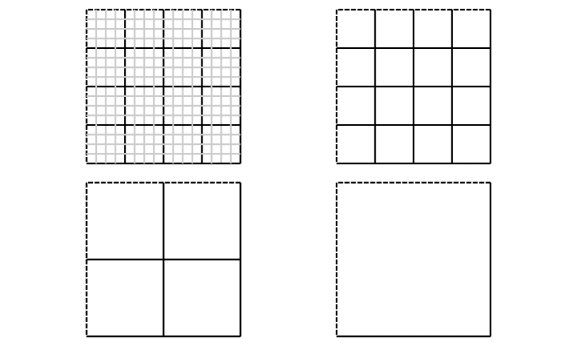
Figure 1. The nested dissection algorithm. The domain is partitioned recursively into smaller square boxes until the side length is equal to a constant $bh$. The algorithm recursively eliminates the interior nodes of a box via Schur complement, combines four boxes into a large one, and repeats the process. The dotted lines stand for the degrees of freedom repeated on the other side of the domain due to periodicity.

Throughout the rest of the paper, we use the nested dissection algorithm to factorize $P$. In this algorithm, the domain $\mathrm{T}^{d}$ is partitioned recursively into square boxes until a certain size $bh$ is reached in each dimension. Each leaf box contains $(b-1)^{d}$ points in its interior and $(b+1)^{d}$ points in its closure. The algorithm then recursively eliminates the interior nodes of a box via Schur complement, combine four boxes into a large one, and repeat. Figure 1 illustrates the nested dissection algorithm in a 2D setting.

An essential observation is that $\mu(j)$ can include more points without affecting much the complexity of the nested dissection algorithm. Let us discuss the 2D case first. At the leaf level, the set $J$ is partitioned into a disjoint union of three types of sets:

• a cell set that contains the $(b-1)^{2}$ interior grid points of a leaf box,

• an edge set that contains the $(b-1)$ grid points at the interface of two adjacent leaf boxes, and

• a vertex set that contains only $1$ grid point at the interface of four adjacent leaf boxes.

The neighborhood $\mu(j)$ of a point $j\in J$ is defined as follows based on the type of the set that contains it:

• for $j$ in a cell set $c$, we set $\mu(j)=\gamma(c)$;

• for $j$ in an edge set $e$, we set $\mu(j)=\gamma(e)$;

• for $j$ in an vertex set $v=\{j\}$, we set $\mu(j)=\gamma(v)$.

In the 3D case, the set $J$ is partitioned into a disjoint union of four types of sets:

• a cell set that contains the $(b-1)^{3}$ interior grid points of a leaf box,

• a face set that contains the $(b-1)^{2}$ grid points at the interface of two adjacent leaf boxes,

• an edge set that contains the $(b-1)$ grid points at the interface of four adjacent leaf boxes, and

• a vertex set that contains only $1$ grid point at the interface of eight adjacent leaf boxes.

For the extra case of $j$ in a face set $f$, we define $\mu(j)=\gamma(f)$.

The second problem is the computation of $Q(j,\mu(j))$. Our choice of the neighborhood shows that $\mu(j)$ is the same for all $j$ in the same (cell, face, edge, or vertex) set. Therefore it is convenient to consider all such $j$ together.

We first fix a cell set $c$ and consider all points $j\in c$. The sparsity condition on $Q$ can be rewritten as

(6) $$Q(c,\gamma(c))G(\gamma(c),\gamma(c)^{c})\approx 0.$$

The rows of the submatrix $Q(c,\gamma(c))$ should also be linearly independent in order for $Q$ to be non-singular. We define $\beta(c)=\gamma(c)\setminus c$, i.e., the set of points that are on the boundary of $c$. Since the matrix $G$ defined in (5) is the Green’s function of a discretized partial differential operator, the rows of $G(c,\gamma(c)^{c})$ can be approximated accurately using the linear combinations of the rows of $G(\beta(c),\gamma(c)^{c})$, i.e., there exists a matrix $T_{c}$ such that

$$G(c,\gamma(c)^{c})\approx T_{c}G(\beta(c),\gamma(c)^{c}).$$

$T_{c}$ matrix can be computed by

$$T_{c}=G(c,\gamma(c)^{c})(G(\beta(c),\gamma(c)^{c}))^{+},$$

where $(\cdot)^{+}$ stands for the pseudoinverse. Finally, we define

$$Q(c,\gamma(c))=\begin{bmatrix}I&-T_{c}\end{bmatrix},$$

assuming the columns are ordered as $(c,\beta(c))$. This submatrix meets the condition (6) and clearly has linearly independent rows. We remark that the computation of $T_{c}$ is the same for any cell $c$ and hence we only need to compute it once.

For a fixed face set $f$, we compute

$$T_{f}=G(f,\gamma(f)^{c})(G(\beta(f),\gamma(f)^{c}))^{+}$$

with $\beta(f)=\gamma(f)\setminus f$ and set

$$Q(f,\gamma(f))=\begin{bmatrix}I&-T_{f}\end{bmatrix},$$

assuming the columns are ordered as $(f,\beta(f))$.

For a fixed edge set $e$, we define

$$T_{e}=G(e,\gamma(e)^{c})(G(\beta(e),\gamma(e)^{c}))^{+}$$

with $\beta(e)=\gamma(e)\setminus e$ and set

$$Q(e,\gamma(e))=\begin{bmatrix}I&-T_{e}\end{bmatrix},$$

assuming the columns are ordered as $(e,\beta(e))$.

Finally, for a fixed vertex set $v$, we let

$$T_{v}=G(v,\gamma(v)^{c})(G(\beta(v),\gamma(v)^{c}))^{+}$$

with $\beta(v)=\gamma(v)\setminus v$ and set

$$Q(v,\gamma(v))=\begin{bmatrix}I&-T_{v}\end{bmatrix},$$

assuming the columns are ordered as $(v,\beta(v))$.

Once the matrix $Q$ has been constructed, the matrix $C$ is computed as follows. For a cell set $c$, we set

$$C(c,\gamma(c))=Q(c,\gamma(c))G(\gamma(c),\gamma(c)),$$

and similarly for a face set $f$, an edge set $e$, and a vertex set $v$. We recall that both $C$ and $P=Q+Cq$ have the same sparsity pattern as $Q$.

2.4. Complexity

We now analyze the complexity of constructing and applying the sparsifying preconditioner. Let $bh$ be the width of the leaf box of the nested dissection algorithm.

In 2D, the construction algorithm consists of two parts: (i) computing the pseudoinverses while forming $T_{c}$, $T_{e}$, and $T_{v}$, and (ii) building the nested dissection factorization for $P$. The former takes at most $O(b^{4}n^{2})=O(b^{4}N)$ steps, while the latter takes $O(n^{3}+b^{6}(n/b)^{2})=O(N^{3/2}+b^{4}N)$ steps. Therefore, the overall complexity of the construction algorithm is $O(N^{3/2}+b^{4}N)$. The application algorithm is essentially a nested dissection solve, which costs $O(n^{2}\log n+b^{4}(n/b)^{2})=O(N\log N+b^{2}N)$ steps.

In 3D, the construction algorithm again consists of the same two parts. The pseudoinverses cost $O(b^{6}n^{3})=O(b^{6}N)$ steps, while the nest dissection factorization takes $O(n^{6}+b^{9}(n/b)^{3})=O(N^{2}+b^{6}N)$ steps. Hence, the overall construction cost is $O(N^{2}+b^{6}N)$. The application cost is equal to $O(n^{4}+b^{6}(n/b)^{3})=O(N^{4/3}+b^{3}N)$ due to a 3D nested dissection solve.

There is a clear trade-off for the choice of $b$. For small values of $b$, the preconditioner is less efficient due to the small support of $Q$, while the computational complexity is low. On the other hand, for large values of $b$, the preconditioner is more effective, but the cost is higher. In our numerical results, we set $b=O(n^{1/2})$. For this choice, the construction and application costs in 2D are $O(N^{2})$ and $O(N^{3/2})$, respectively. In 3D, they are $O(N^{2})$ and $O(N^{3/2})$ as well, respectively.

3. Numerical results

The sparsifying preconditioner, as well as the nested dissection algorithm involved, is implemented in Matlab. The numerical results are obtained on a Linux computer with CPU speed at 2.0GHz. The GMRES algorithm is used as the iterative solver with the relative tolerance equal to $10^{-6}$.

3.1. Helmholtz equation

Two tests are performed for the 2D Helmholtz equation. In the first one the velocity field $c(x)$ is equal to one plus a Gaussian function at the domain center, while in the second test $c(x)$ is given by one plus three randomly placed Gaussian functions. In both tests, the right hand side is a delta source at the center of the domain. The results of these two tests are summarized in Figures 2 and 3. The columns of the tables are listed as follows:

• $\omega/(2\pi)$ is the wave number (roughly the number of oscillation across the domain),

• $N$ is the number of unknowns,

• $b$ is the ratio between the width of the leaf box and the step size $h$,

• $T_{s}$ is the setup time of the preconditioner in seconds,

• $T_{a}$ is the application time of the preconditioner in seconds,

• $n_{p}$ is the iteration number of the preconditioned iteration, and

• $T_{p}$ is the solution time of the preconditioned iteration in seconds.

$\omega/(2\pi)$	$N$	$b$	$T_{s}$(sec)	$T_{a}$(sec)	$n_{p}$	$T_{p}$(sec)
16	$48^{2}$	3	2.5e-01	3.7e-02	7.0e+00	2.1e-01
32	$96^{2}$	6	5.5e-01	2.9e-02	8.0e+00	2.6e-01
64	$192^{2}$	6	2.5e+00	8.1e-02	1.1e+01	1.0e+00
128	$384^{2}$	12	1.2e+01	2.9e-01	2.8e+01	9.8e+00

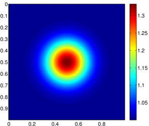
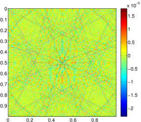
Figure 2. Example 1 of the 2D Helmholtz equation. Top: numerical results. Bottom: $c(x)$ (left) and $u(x)$ (right) for the largest $\omega$ value.

$\omega/(2\pi)$	$N$	$b$	$T_{s}$(sec)	$T_{a}$(sec)	$n_{p}$	$T_{p}$(sec)
16	$48^{2}$	3	2.2e-01	1.3e-02	8.0e+00	1.1e-01
32	$96^{2}$	6	5.0e-01	2.7e-02	1.1e+01	3.8e-01
64	$192^{2}$	6	3.0e+00	7.7e-02	2.1e+01	2.1e+00
128	$384^{2}$	12	1.2e+01	2.9e-01	3.8e+01	1.3e+01

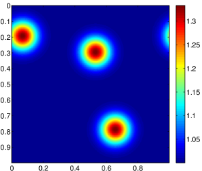
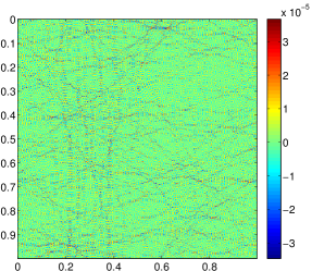
Figure 3. Example 2 of the 2D Helmholtz equation. Top: numerical results. Bottom: $c(x)$ (left) and $u(x)$ (right) for the largest $\omega$ value.

Two similar tests are performed in 3D: (i) in the first one $c(x)$ is equal to one plus a Gaussian function at the domain, and (ii) in the second test $c(x)$ is one plus three Gaussians with centers placed randomly on the middle slice. The right hand side is again a delta source at the center. The results of these two tests are listed in Figure 4 and 5.

$\omega/(2\pi)$	$N$	$b$	$T_{s}$(sec)	$T_{a}$(sec)	$n_{p}$	$T_{p}$(sec)
4	$12^{3}$	3	4.8e-01	1.9e-02	5.0e+00	1.7e-01
8	$24^{3}$	6	6.0e+00	4.7e-02	7.0e+00	3.9e-01
16	$48^{3}$	6	1.5e+02	4.8e-01	8.0e+00	4.0e+00
32	$96^{3}$	12	4.8e+03	7.4e+00	1.0e+01	8.4e+01

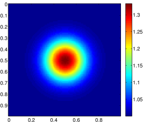
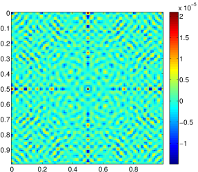
Figure 4. Example 1 of the 3D Helmholtz equation. Top: numerical results. Bottom: $c(x)$ (left) and $u(x)$ (right) for the largest $\omega$ value at the middle slice.

$\omega/(2\pi)$	$N$	$b$	$T_{s}$(sec)	$T_{a}$(sec)	$n_{p}$	$T_{p}$(sec)
4	$12^{3}$	3	3.0e-01	6.5e-03	4.0e+00	2.0e-02
8	$24^{3}$	6	6.3e+00	5.1e-02	5.0e+00	2.9e-01
16	$48^{3}$	6	1.5e+02	4.8e-01	9.0e+00	4.6e+00
32	$96^{3}$	12	4.7e+03	8.4e+00	1.8e+01	1.6e+02

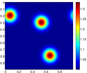
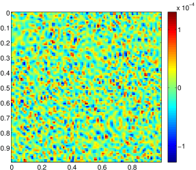
Figure 5. Example 2 of the 3D Helmholtz equation. Top: numerical results. Bottom: $c(x)$ (left) and $u(x)$ (right) for the largest $\omega$ value at the middle slice.

The numerical results in both 2D and 3D examples show that the iteration counts remain quite small even for problems at very high frequency.

3.2. Schrödinger equation

For the numerical tests of (2), we let $\ell=1/h$ and consider

$$(-\Delta+1/h^{2}\cdot V(x/h)-1/h^{2}\cdot E)u(x)=f(x),\quad x\in\mathrm{T}^{d},$$

where $h=1/n$ is again the step size of the pseudospectral grid. The energy shift $E$ is chosen to be equal to 2.5 to ensure that there are about 3 or 4 grid points per wavelength.

Two tests are performed in 2D. In the first one the potential field is an array of randomly placed Gaussians, while in the second one the potential field is given by a regular 2D array of Gaussians with one missing at the center. In both tests, the right hand side is a delta source at the domain center. The results of these two tests are summarized in Figures 6 and 7.

$N$	$b$	$T_{s}$(sec)	$T_{a}$(sec)	$n_{p}$	$T_{p}$(sec)
$48^{2}$	3	2.1e-01	1.3e-02	7.0e+00	1.0e-01
$96^{2}$	6	5.6e-01	2.8e-02	9.0e+00	3.0e-01
$192^{2}$	6	2.5e+00	7.2e-02	2.1e+01	2.1e+00
$384^{2}$	12	1.3e+01	2.1e-01	3.2e+01	9.6e+00

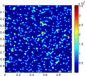
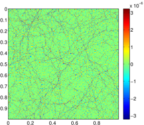
Figure 6. Example 1 of the 2D Schrödinger equation. Top: numerical results. Bottom: $1/h^{2}\cdot V(x/h)$ (left) and $u(x)$ (right) for the largest $N$ value.

$N$	$b$	$T_{s}$(sec)	$T_{a}$(sec)	$n_{p}$	$T_{p}$(sec)
$48^{2}$	3	2.2e-01	1.3e-02	8.0e+00	1.1e-01
$96^{2}$	6	5.0e-01	2.7e-02	1.1e+01	3.8e-01
$192^{2}$	6	3.0e+00	7.7e-02	2.1e+01	2.1e+00
$384^{2}$	12	1.2e+01	2.9e-01	3.8e+01	1.3e+01

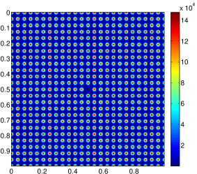
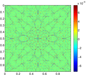
Figure 7. Example 2 of the 2D Schrödinger equation. Top: numerical results. Bottom: $1/h^{2}\cdot V(x/h)$ (left) and $u(x)$ (right) for the largest $N$ value.

Two similar tests are also performed in 3D: (i) in the first one the potential field is equal to an array of randomly placed Gaussians, and (ii) in the second test the potential is a regular 3D array of Gaussians with one missing at the center. The right hand side is still a delta source at the domain center. The results of these two tests are listed in Figure 8 and 9.

$N$	$b$	$T_{s}$(sec)	$T_{a}$(sec)	$n_{p}$	$T_{p}$(sec)
$12^{3}$	3	2.9e-01	6.6e-03	2.0e+00	1.1e-02
$24^{3}$	6	6.0e+00	4.6e-02	9.0e+00	4.8e-01
$48^{3}$	6	1.5e+02	4.3e-01	1.7e+01	8.4e+00
$96^{3}$	12	4.5e+03	8.4e+00	3.1e+01	2.8e+02

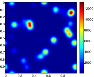
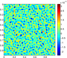
Figure 8. Example 1 of the 3D Schrödinger equation. Top: numerical results. Bottom: $1/h^{2}\cdot V(x/h)$ (left) and $u(x)$ (right) for the largest $N$ value at the middle slice.

$N$	$b$	$T_{s}$(sec)	$T_{a}$(sec)	$n_{p}$	$T_{p}$(sec)
$12^{3}$	3	3.4e-01	7.1e-03	2.0e+00	1.6e-02
$24^{3}$	6	6.1e+00	4.5e-02	5.0e+00	2.5e-01
$48^{3}$	6	1.4e+02	5.0e-01	6.0e+00	3.7e+00
$96^{3}$	12	4.6e+03	7.4e+00	1.2e+01	9.9e+01

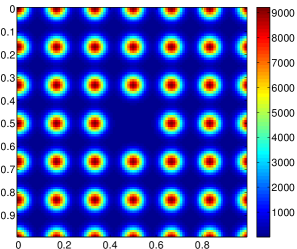
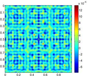
Figure 9. Example 2 of the 3D Schrödinger equation. Top: numerical results. Bottom: $1/h^{2}\cdot V(x/h)$ (left) and $u(x)$ (right) for the largest $N$ value at the middle slice.

In both 2D and 3D examples, the results are qualitatively similar to the ones of the Helmholtz equation. Though the iteration count increases with the system size, it remains quite small even for large scale problems.

4. Conclusion

This paper introduces the sparsifying preconditioner for the pseudospectral approximations of highly indefinite systems on periodic structures. These systems have important applications in computational photonics and electronic structure calculation. The main idea of the preconditioner is to transform the dense system into an integral equation formulation and introduce a local stencil operator $Q$ for its sparsification. The resulting approximate equation is then solved with the nested dissection algorithm and serves as the preconditioner. This method is easy to implement, efficient, and results in relatively low iteration counts even for large scale problems.

In the numerical results, the size $bh$ of the leaf box is of order $O(n^{1/2}h)$. However, the iteration count still grows roughly linearly with $\omega$ (for the Helmholtz equation) and with $1/h$ (for the Schrödinger equation). An important open question is whether other sparsity patterns for $Q$ can result in almost frequency independent iteration counts even for moderate values of $b$.

In computational photonics [joannopoulos-2008], a more relevant equation is the Maxwell equation for the electric field $E(x)$:

$$\left(\nabla\times\nabla\times-\frac{\omega^{2}}{c^{2}}\epsilon(x)\right)E(x)=f(x),$$

where $\epsilon(x)$ is the dielectric function. The sparsifying preconditioner should be extended to this case without much difficulty.

For the density functional theory calculation in computational chemistry, the Schrödinger equation typically has a non-local pseudopotential term in addition to the local potential term in (2). An important future work is to extend the sparsifying preconditioner to address such non-local terms.

The method proposed in this paper provides an efficient way to access a column or a linear combination of the columns of the Green’s function of the operators in (1) and (2). This can potentially open the door for building efficient and data-sparse representations of the whole Green’s function.