A Challenging Solar Eruptive Event of 18 November 2003 and the Causes of the 20 November Geomagnetic Superstorm. IV. Unusual Magnetic Cloud and Overall Scenario

Abstract

The geomagnetic superstorm of 20 November 2003 with Dst = $-422$ nT, one of the most intense in history, is not well understood. The superstorm was caused by a moderate solar eruptive event on 18 November, comprehensively studied in our preceding Papers I – III. The analysis has shown a number of unusual and extremely complex features, which presumably led to the formation of an isolated right-handed magnetic-field configuration. Here we analyze the interplanetary disturbance responsible for the 20 November superstorm, compare some of its properties with the extreme 28 – 29 October event, and reveal a compact size of the magnetic cloud (MC) and its disconnection from the Sun. Most likely, the MC had a spheromak configuration and expanded in a narrow angle of $\leq 14^{\circ}$. A very strong magnetic field in the MC up to 56 nT was due to the unusually weak expansion of the disconnected spheromak in an enhanced-density environment constituted by the tails of the preceding ICMEs. Additional circumstances favoring the superstorm were (i) the exact impact of the spheromak on the Earth’s magnetosphere and (ii) the almost exact southward orientation of the magnetic field, corresponding to the original orientation in its probable source region near the solar disk center.

1 Introduction

S-introduction A series of big eruptive flares in a complex of large super-active regions 10484, 10486, and 10488 occurred late in October 2003 (see, e.g., Veselovsky2004; ChertokGrechnev2005; Gopalswamy et al., 2005a; 2005b; Grechnev2005). These ‘Halloween 2003 events’ produced geomagnetic superstorms with Dst $=-353$ and $-383$ nT on 29 – 31 October. A notable event on 18 November occurred in the decaying active region (AR) 10501 during the second passage across the solar disk of the former AR 10484. This event produced a yet stronger superstorm on 20 November 2003 with Dst $=-422$ nT, the largest one during solar cycle 23 (e.g., Yermolaev2005; Gopal2005c; Yurchyshyn2005; Ivanov2006), and one of the severest storms in history (probably among top ten in terms of the Dst index – see CliverSvalgaard2004).

A number of studies addressed the 18 November 2003 event and its interplanetary consequences, endeavoring to understand its extreme geoeffective impact, but its causes remain unclear. The major outcome of the studies is the oddness of the event, which strongly deviated from the established correlations between solar and near-Earth parameters Yermolaev et al. (2005); Yurchyshyn, Hu, and Abramenko (2005); Srivastava (2005); Chertok et al. (2013). In particular, the magnetic cloud (MC) near the Earth carried an exceptionally strong magnetic field of about 56 nT, while its velocity was modest.

The extreme geomagnetic disturbances of 29 – 30 October and 20 – 21 November (Figure F-cosmice) were produced by solar eruptions from nearly the same complex of active regions (which evolved in the meantime), and therefore one might expect the 18 – 20 November event to inherit the properties of the Halloween events (29 – 30 October). However, it looks instead like their antipode. For example, the 28 October solar event produced large and fast CME and very strong flare emissions in soft X-rays (exceeded the GOES saturation level of X17.2), hard X-rays, and gamma rays; huge radio bursts in microwaves (RSTN radiometers saturated) and up to submillimeters; strong SEP event (Figure F-cosmica), and a ground-level enhancement of the cosmic ray intensity, GLE 65. The 29 October event was similar to the 28 October event. On the other hand, none of the listed extreme properties were found in the 18 November event. It was medium in soft X-rays ($\lsim\,$M5), hard X-rays, and microwaves. The enhancement of the near-Earth proton flux was insignificant (but it could have been reduced due to the easterly position of the active region on 18 November). The associated CMEs had a moderate speed, size, and brightness, and did not exhibit any extreme features. The time intervals between the solar eruptions and the geomagnetic storm onset/peak times were 19/38 h on 29 October and much longer on 20 November, 48/61 h.

Figure 1.: Solar protons (a), galactic cosmic ray data (b – d, Courtesy V. Sdobnov), and geomagnetic disturbances (e) during the late October through November interval. The spherical harmonics of the galactic cosmic ray pitch-angle anisotropy are shown in panel c (first harmonic, $A_{1}$) and d (second harmonic, $A_{2}$). The dashed lines mark the 28 October and 18 November solar events. F-cosmic

The peculiarities are also related to the MC, which reached the Earth’s magnetosphere on 20 November. The $z$-component of the magnetic field ($B_{z}$) in the MC was pointed southward (negative), although the MCs produced by the eruptions from AR 10484 in October had positive $B_{z}$. The magnetic helicity of the MCs responsible for the Halloween superstorms (from AR 10486) was negative, but it was positive in the MC of 20 November. Moreover, the orientation and handedness of the magnetic field in the 20 November MC mismatched those in its presumable source region AR 10501 Möstl et al. (2008); Chandra et al. (2010).

Thus, the extremely geoeffective event of 18 – 20 November has offered four major problems: (i) incomprehensible causes of its extremeness, (ii) its enigmatic solar source, and perplexing (iii) orientation and (iv) handedness of the magnetic field in the MC. Despite several ideas proposed in the listed studies to address these issues, satisfactory explanations are still missing. This enigmatic event offers the challenge in predictions of geomagnetic disturbances that can occur unexpectedly and can be destructive for modern and future high-technology societies.

These circumstances were the major reasons that inspired us to undertake a comprehensive analysis of this event presented in our Paper I Grechnev et al. (2014a), Paper II Grechnev et al. (2014b), and Paper III Uralov et al. (2014). The analysis has revealed an extremely complex, unusual solar eruptive event. None of the observed CMEs was an appropriate candidate for the source of the MC, being only able to produce a glancing blow on the Earth due to their rather large angles with the Sun – Earth line. However, three different reconstructions of the MC Yurchyshyn, Hu, and Abramenko (2005); Möstl et al. (2008); Lui (2011) showed its central encounter with Earth.

On the other hand, indications were found of an additional eruption, which probably occurred rather far from AR 10501 but close to the solar disk center. The presumable erupted magnetic structure was a right-handed pair of linked tori moving away from the Sun, and slowly expanding with a radial (lateral) speed of $\approx 100$ km s^-1, i.e., within a narrow angle of $\lsim 14^{\circ}$ (Papers II and III). It is not completely clear into what structure the couple of tori evolved. Most likely, this structure was disconnected from the Sun and developed into a toroid (donut-shaped) or spheromak (spherical, no central hole). Due to its weak expansion, the earthward direction of propagation, and a presumably small mass, the probability to detect this eruption in coronagraph images was very low. Therefore this eluding structure could have evolved into the MC that reached Earth on 20 November.

We will not list all the ideas proposed previously and follow instead only those results and suggestions that appear to be consistent with these findings and promising to shed light on the issues in question. The major reasons for the superstorm of 20 November 2003 were the strongest magnetic field in the MC (close to a record value, while its speed was ordinary) and its orientation ($\theta=-(49-87)^{\circ}$; see Moestl2008). Qiu2007 demonstrated a quantitative correspondence between the magnetic fluxes in nine MCs and their solar source regions. Furthermore, Chertok2013 analyzed the major geomagnetic storms (Dst $<-100$ nT) in solar cycle 23 whose solar source regions were located with sufficient reliability in the central part of the disk. They found that the intensity of the geomagnetic storms, as well as the ICMEs’ Sun–Earth transit times, were mainly governed by the parameters of their solar sources, such as the total unsigned magnetic flux at the photospheric level within the post-eruption EUV arcades and dimming regions. For example, the magnetic fluxes in the solar sources of the strongest geomagnetic storms in cycle 23 ($\mathrm{Dst}<-200$ nT, the near-Earth magnetic field $|{\bf B}|>50$ nT, and large southern $B_{z}$ component) such as the 14–15 July 2000, 22–24 November 2001, 28–30 October 2003, and 13–15 May 2005 superstorms (see, e.g., Wu2005; Cerrato2012; Manchester2014) were very large, $(240-870)\times 10^{20}$ Mx (maxwell). The severity of the geomagnetic superstorm of 20 November 2003 appears to correspond to the near-Earth magnetic field of $|{\bf B}|_{\max}\approx 56$ nT with a large southward component up to $B_{z}\approx-45$ nT, while the total unsigned magnetic flux in the eruption region was as low as $130\times 10^{20}$ Mx, even including the flare arcade in AR 10501 and all dimming regions. The only way to get an extremely strong magnetic field with a modest magnetic flux is a small size of the MC. This conjecture is consistent with the above-mentioned reconstructions of the MC, all of which showed both its dimensions in the ecliptic plane to be $<0.3$ AU ($<17^{\circ}$). One more indication is that the Forbush decrease (FD) on 20 November was much less than that after the 28 October event. Note also the idea about the compression of the MC due to the interaction among CMEs Gopalswamy et al. (2005c); Yermolaev et al. (2005).

The mentioned reconstructions were based on the fitting of specific configurations such as a torus or cylinder Yurchyshyn, Hu, and Abramenko (2005); Möstl et al. (2008); Lui (2011); Marubashi et al. (2012) to the observed rotating magnetic components in the MC. The fitted components more or less resembled the observed ones within some limited portions of the ICME, overlapping with each other, but covering somewhat different parts of the ICME in different reconstructions. On the other hand, considerations of the $\phi_{B}$ and $\theta_{B}$ angles led KumarManoUddin2011 to the idea that the MC occupied a longer part of the ICME along the Sun–Earth line (see also Gopal2005c and Marubashi2012). This possibility suggests that its magnetic structure might be different from those considered previously.

To verify these suggestions and shed further light on the enigmatic 18 – 20 November 2003 event, we address the corresponding ICME here. In Section S-icme we revisit in situ measurements of the interplanetary disturbance, analyze ground-based data on cosmic rays, and consider heliospheric three-dimensional (3D) reconstructions made from the observations of the Solar Mass Ejection Imager (SMEI; Eyles2003; Jackson2004). Then we discuss the results and their implications in Section S-discussion. In particular, we endeavor to understand the probable causes of the superstorm, to follow the whole presumable chain of events from the solar eruption on 18 November up to the encounter of the MC with the Earth on 20 November, and to outline possible ways to diagnose such anomalously geoeffective events.

2 Properties of the ICME

S-icme As mentioned above, the 20 November geomagnetic superstorm was a conspicuous exception to almost all established statistical correlations (see, e.g., Yurchyshyn2005; Srivastava2005; Chertok2013). What is surprising is that it also promises an opportunity to find hints on the causes of the superstorm from its peculiarities. By comparing the 28 October event and related interplanetary disturbances with those of 18–20 November, we hope to understand the incomprehensibly large geomagnetic effect of the 18 November eruption.

2.1 Interplanetary Data

Data on in situ measurements of the interplanetary disturbance have been addressed in several studies (e.g., Yurchyshyn2005; Yermolaev2005; Gopal2005c; Moestl2008; KumarManoUddin2011; Marubashi2012). Nevertheless, some significant particularities in this event were not discussed previously. Here we consider the near-Earth ICME observations made with Solar Wind Electron Proton Alpha Monitor (SWEPAM; McComas1998) and Magnetometer Instrument (MAG; Smith1998) on Advanced Composition Explorer (ACE). Figure F-ace shows records of the magnetic field components $B_{x}$, $B_{y}$, and $B_{z}$ along with a magnitude $|{\bf B}|$ (a), solar wind velocity (b), proton temperature (c) and density (e), and plasma $\beta$ value inferred from the above parameters.

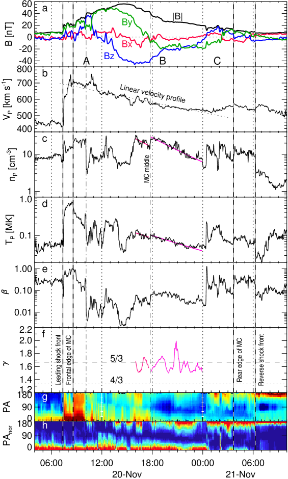
Figure 2.: ACE data. (a) $B_{x}$, $B_{y}$, and $B_{z}$ components of the magnetic field and its magnitude $|{\bf B}|$. Parameters of the ejecta: velocity (b), proton density (c) and temperature (d), and plasma $\beta$ value (e). (f) Polytropic index $\gamma$ inferred from the density and temperature in two intervals marked with the pink and purple lines. (g) Pitch angle distribution of 272 eV electrons (minimum blue, maximum red). (h) Same as (g) but with a moving normalization (adopted from Marubashi et al., 2012).F-ace

The identification of the boundaries of the magnetic cloud was made as follows. After the arrival of the shock front at about 07:20 UT on 20 November, the plasma velocity kept on increasing up to the contact surface that is typical of a bow shock. This fact suggests significance of the aerodynamic drag. The thick dashed line at 08:35 and the thin dash-dotted line at 10:08 in Figure F-ace mark a possible arrival time of the MC frontal edge, but this is rather uncertain. The earlier thick line roughly corresponds to the position of the highest plasma velocity. Such a situation occurs at the forward stagnation point of a supersonic body with fixed shape and size. The later thin line approximately corresponds to the position where the plasma beta and density underwent a seemingly sharp drop. This situation is expected for a typical MC. It is difficult to choose between the two options of the MC leading edge for the following reasons. On the one hand, the MC must have expanded with a velocity of the order of 100 km s^-1 which was appreciably higher than the fast-mode speed in the undisturbed solar wind and would have prevented a stationary flow around the ICME. On the other hand, the nearly self-similar expansion of a MC that is often assumed implies conservation of the profile of the plasma beta formed at the MC creation. As Paper III showed, the MC hitting the Earth was probably formed from multiple magnetic structures with considerably different temperatures, densities, and possibly plasma beta values. Therefore, sharp changes in plasma beta value without significant variations in $|{\bf B}|$ in Figure F-ace might correspond to these different parent structures.

We consider the first thick dashed line as the leading edge of the MC because of (i) equality of the $B_{z}$ flux in a closed magnetic structure (see below), (ii) a sharp density increase in suprathermal electrons (Figure F-aceg) discussed later, and (iii) sharp changes in the proton temperature and density. The conditions (i) and (iii) were also used in identifying the rear edge of the MC.

One more feature deserving attention is a weak reverse shock in Figure F-ace at 06:10 on 21 November. Its presence as well as the presence of the forward shock indicates that the expansion of the MC was not free for all directions. A reverse shock can be due to two reasons. One is overexpansion of the MC if its earthward bulk velocity was less than the velocity of its own expansion. This was not the case here. The second possibility for the development of the reverse shock appears if the MC was pressed from behind by the faster flow of the disturbed solar wind. The latter situation is favored if the MC was disconnected from the Sun. In this situation the MC would not have been protected from lateral disturbances such as shocks and related high-speed flow which could come from expanding CME1, CME2, and CME3. If the magnetic flux rope was connected to the Sun, then the extended magnetic structure would have protected the top of the MC from such lateral disturbances.

The trend of the velocity in the MC (region B in Figure F-acea) is close to a linear one (dotted line), which is an attribute of a self-similar expansion Low (1984). Such expansion occurs if all forces affecting the ejecta (magnetic forces, plasma pressure, and gravity; so far we have neglected the aerodynamic drag because its effect is not self-similar) decrease with distance by the same factor Low (1982); Uralov, Grechnev, and Hudson (2005). This condition is satisfied if the polytropic index of the MC gas is $\gamma=4/3$. Its actual value in the MC interior can be estimated from the proton density and temperature (Figures F-acec and F-aced) as $\gamma=n/T\,\left(dT/dt\right)/\left(dn/dt\right)+1$ as shown in Figure F-acef. This expression is valid if the entropy distribution inside the MC is uniform. Averaging of values obtained in this way provides an average $\gamma$ inside the MC. To suppress fluctuations in the computation of the derivatives, we fitted the trends within two intervals with smooth functions (pink and purple). The actual $\gamma$ varies around $5/3$; the difference from $4/3$ does not seem to be significant, because $\beta\leq 0.1$ within this interval. (According to Farrugia1995, the estimated value of $\gamma$ supports the spheromak configuration rather than a flux rope.) These circumstances allow us to calculate an expansion-corrected ‘snapshot’ of the ICME assuming its expansion to be exactly self-similar. We infer the time-dependent expansion factor $\xi(t)$ from the linear fit to the velocity profile. The correction factor for the magnetic field strength in the snapshot related to moment $t_{0}$ is $[\xi(t_{0})/\xi(t)]^{2}$ (from the magnetic flux conservation), and the correction factor for the density is $[\xi(t_{0})/\xi(t)]^{3}$.

Figures F-ace_cor_spheromaka and F-ace_cor_spheromakb show such ‘snapshots’ for the magnetic field and density distributions in the ICME along the Sun – Earth line corresponding to the first contact with the ACE spacecraft. The expansion factor evaluated from the linear velocity profile in Figure F-aceb was squared and applied to the magnetic field strength; likewise it was cubed and applied to the density. The total length of the ICME in the Sun – Earth direction was $\approx 0.22$ AU and, according to the reconstructions of the MC Yurchyshyn, Hu, and Abramenko (2005); Möstl et al. (2008); Lui (2011), its axis passed close to the ACE spacecraft.

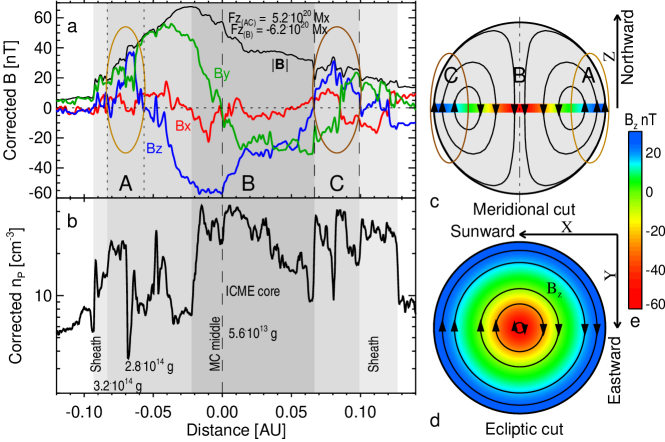
Figure 3.: A ‘snapshot’ of the magnetic field (a) and density (b) distributions in the ICME along the Sun–Earth line according to the expansion-corrected ACE data. The ICME size corresponds to the first contact with ACE. (c, d) A magnetic configuration of a perfect spheromak with its axis shown perpendicular to the ecliptic plane for simplicity. The brown ovals outline the regions presumably belonging to the leading (A) and trailing (C) parts of the MC. (e) The color scaling of the $B_{z}$ component in a perfect spheromak shown in panels (c) and (d) and roughly corresponding to $-B_{z}$ in Figure 15 of Lui (2011). F-ace˙cor˙spheromak

The behavior of the $B_{x}$ component, which alternately reached significant positive and negative values within the MC (see also Figure 12 in Lui2011), rules out a glancing blow of the flux rope connected to the Sun; otherwise, the sign of $B_{x}$ would not change in the MC. Variations in the magnetic components in regions A and C outlined with the brown ovals in Figure F-ace_cor_spheromaka look like their regular continuations from region B rather than piled-up fluctuations in the sheath. To verify this conjecture, we estimated the total magnetic fluxes of the $B_{z}$ component in region B, on the one hand, and the corresponding sum in regions A and C, on the other hand, assuming the ICME cross section to be circular. To take account of the ICME asymmetry in the Sun–Earth direction, the two estimates for each ICME half were averaged. The result shown in Figure F-ace_cor_spheromaka demonstrates that the difference between the magnetic fluxes in regions B ($-6.2\times 10^{20}$ Mx) and A+C ($5.2\times 10^{20}$ Mx) did not exceed 20%. These values are close to the estimate of $5.5\times 10^{20}$ Mx obtained by Moestl2008, despite the coarseness of our approach. Hence, the magnetic field variations in regions A and C were, most likely, not sporadic.

The presence of the opposite magnetic $B_{z}$ components and the equality of their fluxes together with the same situation for $B_{y}$ (while $B_{x}$ was rather small) indicate their balance in the ICME, i.e., a closed magnetic field in the MC. This is only possible if the MC was not connected to the Sun, so that its configuration was either an isolated toroid or a spheromak. In either case, the angle between the MC axis and the ecliptic plane must be large. We adopt the spheromak configuration and later confirm this assumption by different indications considered in Section S-icme.

A simplest 2.5-dimensional configuration which satisfies the equality of magnetic fluxes is an infinitely long cylinder with a linear force-free magnetic field inside: $B_{z}=J_{0}(\alpha r),B_{\varphi}=\sqrt{(B_{x}^{2}+B_{y}^{2})}=J_{1}(\alpha r)$ where $J_{n}$ is the Bessel function of order $n$. The boundary of the cylinder is determined by the first root of the equation $J_{1}(\alpha r)=0$. The total magnetic flux through the normal cross section of such a magnetic flux rope is zero. A 3D analog of this situation is a spheromak whose total magnetic flux equals to zero in both equatorial and meridional cross sections. The boundary of a spheromak is determined by the first root of the equation $j_{1}(\alpha r)=0$ where $j_{1}$ is the spherical Bessel function of order 1. A transformation of a long cylindric flux rope into a thin toroid does not significantly change the inherent situation for an infinitely long flux rope. A force-free flux rope whose small radius is determined by the condition $J_{1}(\alpha r)=0$ cannot have its footpoints in the solar surface. If it were so, then the total magnetic flux in each photospheric footpoint of the flux rope would be zero, which obviously disagrees with observations of eruptive coronal flux rope structures. Thus, the MC was most probably a force-free self-closed magnetic structure rather than that connected to the Sun, and the total magnetic flux in its cross section was zero.

It is important to note that usually the boundary of a MC is considered as the surface on which the axial magnetic field of either a loop-like flux rope or toroid is zero. The linear force-free approximation in this situation corresponds to the equation $J_{0}(\alpha r)=0$ whose first root determines the boundary of a rope. In this case, the total flux of the axial magnetic field in the flux rope’s cross section is maximum but not zero. At present this scheme is a basis of the technique to fit the internal magnetic structure of many observed MCs (see, e.g., RomashetsVandas2003; MarubashiLepping2007). Marubashi2012 also employed this technique to determine the geometry of the 20 November 2003 MC. However, this technique does not permit the presence of the opposite magnetic $B_{z}$ components with the equality of their fluxes that we emphasize. The fitting technique usually employed is not usable in the 20 November 2003 event exactly for this reason.

A quite different Grad – Shafranov reconstruction technique was used by Yurchyshyn2005, Moestl2008, and Lui2011. This technique allows one to reconstruct a two-dimensional cross section of a MC and to evaluate the inclination of its axis only if the MC is a nearly straight portion of a magnetic flux rope with the curvature, plasma pressure, and magnetic field slowly varying along the flux rope axis. Regrettably, the reconstruction intervals in these papers did not fully cover all the three intervals A, B, and C shown in Figure F-ace_cor_spheromak. Moestl2008 considered a large portion of interval B starting from its earlier boundary. Yurchyshyn2005 included the same portion and a half of interval A. Lui2011 considered the whole interval B and almost the whole interval C. Nevertheless, Figure 15 from Lui2011 shows that the direction of the ${\bf B}_{x}+{\bf B}_{y}$ vector is practically constant from the flux rope center to its periphery despite the change in sign of $B_{z}$. The ecliptic cut of the spheromak in Figure F-ace_cor_spheromakd shows the same situation. A cut of a force-free magnetic cylinder with a boundary determined by the condition $J_{1}(\alpha r)=0$ is similar. However, one should be aware of the fact that the results of the Grad – Shafranov reconstruction of the outer part of a MC can be distorted if all the MC dimensions are comparable which is the case for a spheromak. Possibly, this circumstance was responsible for the appearance of an X-point in the reconstruction of Yurchyshyn2005.

Figures F-ace_cor_spheromakc and F-ace_cor_spheromakd show two views of a perfect non-distorted spheromak with its axis perpendicular to the ecliptic for simplicity. The regions outlined with the ovals correspond to regions A (dark brown ovals) and C (bright brown ovals) in Figure F-ace_cor_spheromaka. The passage of the spheromak across the ACE spacecraft is expected to produce a response that is close to the observed one. The actual front/tail asymmetry of the magnetic field indicates compression of the leading half of the MC and stretch of the trailing one, suggesting a significant role of the aerodynamic drag. Note that the toroidal (Figure F-ace_cor_spheromakd) and poloidal (Figure F-ace_cor_spheromakc) magnetic fluxes in the spheromak are transposed with respect to a torus (connected to the Sun or disconnected).

For a spheromak configuration it is possible to estimate the total mass of the ICME. We consider a simple three-layer spheroid consisting of (i) a central core, (ii) the middle portion, and (iii) a sheath. The ICME cross section is assumed to be an oval extending along the Sun-Earth line with an eccentricity of 2 according to Moestl2008. The estimates for the leading and trailing halves of the MC are averaged. The results are shown in Figure F-ace_cor_spheromakb for the three layers separately. The total ICME mass is estimated to be $\lsim 10\times 10^{14}$ g and, since the sheath mass was acquired by the ejecta on the way to the Earth, the initial mass of the CME was, most likely, $\lsim 5\times 10^{14}$ g. This estimate is consistent with the conclusion of Paper I that the major part, $(2-4)\times 10^{15}$ g, of the initial mass of the eruptive filament of $(4-6)\times 10^{15}$ g remained on the Sun.

Figure F-ace shows that the standoff distance between the ICME piston and the shock ahead was $\approx 0.02$ AU, significantly less than a typical value of 0.1 AU Russell and Mulligan (2002). According to the formulas given in this reference, the radius of curvature of the ICME nose in this case must be $\lsim 0.1$ AU for each of the $X$ and $Y$ ICME dimensions with any Mach number $M>1$. This radius of curvature is consistent with the ICME geometry discussed in the preceding paragraph and the conclusion of Vandas1997 related to a spheromak.

The spheromak configuration of the MC addresses the suggestions of its small size mentioned in Section S-introduction. The length of the MC along the Sun-Earth line (the $X$-direction) was about 0.2 AU (see Figure F-ace_cor_spheromak). The $Y$-size was close to the $X$-size, as the reconstructions of the MC presented by Yurchyshyn2005, Moestl2008, and Lui2011 showed indeed. Considering all the facts, we have to conclude that the whole spheromak-shaped ICME expanded within a narrow cone of $\leq 14^{\circ}$. Therefore, the corresponding CME could appear from behind the occulting disk of LASCO/C2 at distances $\geq 16R_{\odot}$, where the Thomson-scattered light was meager. Such a CME could only be detected with LASCO if its mass were very large, which was not the case. It is therefore not surprising that nobody has succeeded in detecting this CME in LASCO images.

We have concluded that the magnetic configuration of the MC was closed, i.e., the MC acted as a trap for charged particles. This suggestion can be verified by considering the pitch-angle distribution of suprathermal electrons. Manifestations of bidirectional streams in pitch-angle maps are sometimes considered as evidence for the connection of a MC to the Sun, as Moestl2008 did. However, bidirectional particle streams are not exclusively produced by mirror reflections at the footpoints of a magnetic flux rope anchored on the Sun. For example, closed isolated torus or spheromak configurations are perfect magnetic traps, and therefore bidirectional particles can also be present in such configurations. Thus, we agree with the approach of Marubashi2012 who revealed the presence of counter-streaming electrons during more than half a day on 20 – 21 November and considered them among indications of a closed MC structure.

The pitch angle distribution of electrons in the 272 eV channel calculated by Marubashi2012 as 5-min averages normalized to the maximum flux value in each time bin is shown in Figure F-aceh. To understand the nature of the bidirectional electron flows, let us consider the records of the $B_{x}$ and $B_{y}$ components shown in Figures F-acea and F-ace_cor_spheromakb (see also Figure 12 of Lui2011). Before the arrival of the MC, the signs of these magnetic components were $B_{x}<0,B_{y}>0$, and after the departure of the MC $B_{x}>0,B_{y}<0$, suggesting that the MC passed the ACE spacecraft when it crossed a sector boundary of the heliospheric magnetic field (anti-sunward before the MC and sunward afterwards; see also Ivanov2006). This orientation corresponded to small pitch angles of electrons flowing away from the Sun before the MC and those close to $180^{\circ}$ after the MC passage as seen in Figure F-aceh. The bidirectional electron flows might have appeared due to the reconnection of the MC with the surrounding magnetic fields, which is supported by a nearly linear trend separating the electron pitch-angle distribution. The trend implies a gradual change in the predominant reconnection at one MC edge to the opposite one as the MC passed through the sector boundary. Thus, the bidirectional electron flows might have been absent in the MC without reconnection, and therefore should not be considered in favor of the connection of the MC to the Sun.

An additional indication of the trap-like behavior of the MC can be revealed from the pitch-angle distribution of the 272 eV electrons with an overall normalization presented in Figure F-aceg. Region A of the ICME presumably belonged to the MC. Indeed, the SWEPAM-E plot shows a sharp increase in the electron density at the leading MC boundary, which we identified, and saw no drastic changes afterwards.

In contrast to the considered indications of the unusual spheromak configuration of the 20 November 2003 MC, the Halloween 2003 MC showed the properties typical of a classical croissant-like flux rope. The latter event and its solar source were addressed by Yurchyshyn2005.

2.2 Data on Heavy Relativistic Particles

The intensity of geomagnetic storms is known to strongly depend on the parameters (the sign and value of the $B_{z}$ component, speed) in a relatively local ICME part interacting directly with the Earth’s magnetosphere (see, e.g., TsurutaniGonzalez1997), while the depth of FD is determined by global characteristics of an ICME, particularly such as its magnetic field strength, size, and speed (see, e.g., Belov2009). Figure F-cosmice shows that the geomagnetic effect from the 18 November event (in terms of the Dst index) was stronger than that of the 28 October event, but the FD from the 20 November interplanetary disturbance was incomparably moderate with respect to the huge Halloween event (Figure F-cosmicb). However, such a comparison of FDs in the two events may not be adequate. In particular, the 29 October FD was the largest one ever observed with neutron monitors Belov (2009) and could acquire its value only due to an extremely rare combination of circumstances.

For comparison with other events we have used a data base on interplanetary disturbances and FDs created in IZMIRAN (Belov et al., 2001, 2009). The density variations of cosmic rays in the data base refer to cosmic rays of 10 GV rigidity, which is close to the effective rigidity for the majority of ground-based neutron monitors, so that cosmic ray variations around this rigidity can be evaluated with a highest accuracy. The FD magnitude determined in this way was 28.0% for 29 October FD and 4.7% for 20 November. The latter magnitude was probably underestimated and needs correction for the following reasons. An unusually large magnetospheric variation in the cosmic ray intensity observed with ground-based detectors on 20 November resulted in a decrease in the geomagnetic cutoff rigidities at observation stations Belov et al. (2005) which reduced the FD depth evaluated over the worldwide neutron monitor network. Thus, the real magnitude of the 20 November FD was most likely 6 – 7%; this has been really confirmed by the most recent estimate of 6.6% by taking account of the magnetospheric effect. This effect is generally large Belov et al. (2001), but does not seem to correspond to the parameters of the associated ICME. With a strength of the total interplanetary magnetic field $|{\bf B}|$ of up to 55.8 nT (hourly averages), one might expect a considerably larger FD, because such a strong magnetic field was observed only twice over the whole history of the solar wind observations. The two other events that occurred in November 2001 had the corresponding FDs with considerably larger amplitudes, 9.2% and 12.4%. All but one (31 March 2001) event with strongest magnetic field exceeding 45 nT caused FDs larger than that of 20 November (pronouncedly larger, as a rule).

Besides the magnetic field strength in an ICME, the solar wind speed should be taken into account in these comparisons. Unlike the magnetic field, the solar wind speed on 20 November was ordinary and increased only up to 703 km s^-1 (hourly data). The FD magnitude is known to correlate well with the product of the observed maximum magnetic field strength $|{\bf B}|_{\max}$ and the solar wind speed $V_{\max}$ (e.g., Belov2009). In the 20 November 2003 event, the $|{\bf B}|_{\max}V_{\max}$ product normalized to 5 nT and 400 km s^-1 is 19.6, while the whole range of the product over the data base is from 0 to 29.6. We have considered all the events with $|{\bf B}|_{\max}V_{\max}>15$ that were not influenced by preceding events. Almost all the events (except for the mentioned 31 March 2001 event) produced deeper FDs than the 20 November 2003 one, with an average value of $10.1\pm 1.8\%$. This value is probably underestimated, because data on the solar wind were incomplete or absent during several largest FDs. Due to this reason, our sample does not include such FDs as those in August 1972 (25%) and in October 2003 (28%).

Thus, the ICME parameters observed on 20 November 2003 suggested expectations of a larger FD. This fact implies that a smaller size and/or an unusual structure of the CME in question can be a reason for its lowered ability to modulate cosmic rays. It is possible that two kinds of powerful CMEs/ICMEs exist whose different structure and other properties produce the difference between their influence on cosmic rays even with equal parameters of the plasma velocity and magnetic field strength.

Both the geomagnetic effect and FD of an ICME are considered to depend on parameters of a MC with the FD depth being independent of $B_{z}$; thus, the inconsistency between the geomagnetic effect and the FD depth provides further support to the small size of the 20 November MC. Indeed, its extent along the Sun – Earth line was about a factor of three smaller than that of the Halloween MC, and reconstructions of the MC Yurchyshyn, Hu, and Abramenko (2005); Möstl et al. (2008); Lui (2011) show its perpendicular size in the ecliptic to be even less than the Sun – Earth extent. Thus, the cross-sectional area of the 20 November MC was one order of magnitude smaller than that of the 28 October MC.

An additional indication can be revealed from the pitch-angle anisotropy of relativistic protons. Their gyroradius is larger than that of suprathermal electrons by a factor of $\approx 10^{5}$, which considerably reduces effects on their pitch-angle anisotropy due to factors irrelevant to trapping. Therefore, anisotropy of relativistic protons promises still more reliable indication of a large-scale magnetic trap connected to the Sun than low-energy electrons do. Anisotropy appears in ground-level enhancements of cosmic ray intensity (GLE events) and due to modulation of galactic cosmic rays by magnetic clouds and corotating interacting regions in the solar wind.

The spherical harmonics of the pitch-angle anisotropy computed by Dvornikov2013 from the data of the worldwide neutron monitor network using the method of Dvornikov and Sdobnov (1997; 1998) are shown in Figures F-cosmicc (first harmonic, $A_{1}$) and F-cosmicd (second harmonic, $A_{2}$). The percentage in the figure shows the excess of the cosmic ray intensity over the opposite direction (100% correspond to a two-fold excess). The second harmonic of the pitch-angle distribution of 4.1 GeV protons indicates that their trapping was absent just before 20 November, while the first harmonic was well pronounced, unlike the end of October, when both harmonics were distinct.

Richardson2000 showed that significant increases in the second harmonic of the cosmic ray anisotropy corresponding to bidirectional particle flows are typical of MCs of large ICMEs. An example is shown by the ICMEs of 29 and 30 October in Figure F-cosmic. In addition to the incompatibly moderate FD with respect to very large Dst, the absence of any increase in the second harmonic on 20 November clearly indicates that this ICME was unusual.

2.3 Heliospheric 3D Reconstructions from SMEI Observations

While the CME of interest is not detectable in SOHO/LASCO images, now we consider 3D reconstructions of heliospheric disturbances made from white-light Thomson scattering observations with SMEI. Three SMEI cameras allow us to achieve a combined $\approx 160^{\circ}$ wide field of view at a sufficiently high spatial resolution. The tomographic reconstructions have been made by the Center for Astrophysics and Space Sciences in University of California, San Diego (CASS/UCSD).

Figure F-smei presents 3D reconstructions from SMEI data of the heliospheric response for two ICMEs ejected on 28 October (upper row) and 18 November 2003, which we want to compare. The images show heliospheric plasma density distributions as viewed from 3 AU, $30^{\circ}$ above the ecliptic plane and $\approx 45^{\circ}$ west of the Sun–Earth line. The location of the Earth is indicated by a blue circle with the Earth’s orbit viewed in perspective as an ellipse. The Sun is indicated by a red dot. An $r^{-2}$ density gradient is removed.

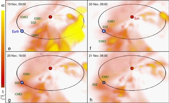
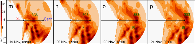
Figure 4.: SMEI 3D reconstructions made by the CASS/UCSD team. (a – d) Large croissantshaped ICME observed on 29 – 30 October suggesting a flux rope connected to the Sun (from Jackson et al., 2006). (e – h) Ejecta observed on 19 – 21 November: ICME1, ICME2, ICME3, and a probable compact source of the geomagnetic storm (SGS). (i – l) Ecliptic and (m – p) meridional cuts corresponding to the remote views (e) – (h). Here ‘IR’ means a probable intrusion region of CME2 into CME1. The scale bars on the left quantify the densities in the corresponding rows. F-smei

Figures F-smeia –F-smei d adopted from Jackson2006 show four successive times of the heliospheric response to the 28 October CME. The images reveal a large croissant-shaped ICME expanding from the Sun and suggest connection of the flux rope to the Sun. The overall picture shows a presumably typical scenario: a large expanding flux rope reached the Earth on 29 October and caused (with its southern $B_{z}$) the severe geomagnetic storm.

The SMEI 3D reconstructions for the 18 – 20 November event in Figures F-smeie –F-smei h present a very different picture, which is more complex (see also the movie SMEI˙19-20˙11˙2003.mpg accompanying the electronic version of the paper). To make it clearer, Figures F-smeii –F-smei l also show the corresponding ecliptic cuts, and Figures F-smeim –F-smei p show the meridional cuts. A comparison between the heliospheric disturbances within a sector of $\approx 120^{\circ}$ embracing the Earth, on the one hand, and the CMEs observed by LASCO on 18 November by taking account of their directions and speeds (see Paper II), on the other hand, allows one to presumably identify visible ICMEs with the southeast CME1 and southwest CME2 as was addressed in Paper II. They are labeled ICME1 and ICME2. An extended density enhancement labeled ICME3 in Figure F-smeie appears to correspond to the fastest far-east CME3.

A far-west Y-like feature resembles in shape the darkening observed with CORONAS-F/SPIRIT at 304 Å (see Paper I). However, the speed of the 304 Å darkening was only $\lsim 100$ km s^-1, which rules out their association.

A large inhomogeneous density enhancement (IR) south of the ecliptic, which is visible in the meridional cuts (Figures F-smeim –F-smei p) as a multitude of small blobs, appears to correspond to the region where CME2 intruded into CME1 (see Paper II). The intrusion region appears to have missed the Earth being south of it.

A feature of our major interest is a rather compact blob exactly impacting the Earth, in which is a moderate density enhancement presumably associated with the source of the geomagnetic storm (SGS). The passage of the blob across the Earth temporally corresponded to the ACE measurements (Figure F-acec). The maximum density in the lower-resolution SMEI two-dimensional cuts passed through the Earth at about 00 UT on 21 November (i.e., between Figures F-smeik and F-smeil) which reasonably corresponds to the weighted center of the expansion-corrected higher-resolution ACE record in Figure F-ace_cor_spheromakb (before the density minimum at the end of the ICME core, cf. Figure F-acec). The SGS dimensions correspond to expectations: the dotted lines in Figures F-smeii –F-smei l delimit a sector of $14^{\circ}$ where the bulk of the ICME mass was concentrated. The images do not leave any doubt that just this blob was associated with the MC responsible for the geomagnetic disturbance.

The density in the blob was moderate, peaking at 22 cm^-3 according to the SMEI tomography, which is close to the ACE measurements. The blob was surrounded by a larger enhanced-density cloud suggesting a possible influence from the southwestern ICME2 and southeastern ICME1 as well as the southern intrusion region. As all the three representations of the SMEI reconstructions show, the shape of the blob suggest neither a larger isolated torus nearly perpendicular to the ecliptic plane nor a croissant connected to the Sun. The spheromak configuration appears to be most appropriate. Thus, the SMEI data put the last missing point in hunting out the mysterious source of the 20 November superstorm.

3 Discussion

S-discussion All the observational facts and indications considered in Section S-icme lead to the conclusion that the 20 November MC was a spheromak of a small size disconnected from the Sun. These peculiarities of the 20 November ICME must be reflected in its propagation between the Sun and Earth. Let us compare the corresponding properties of the 18 November and 28 October ICMEs.

3.1 Propagation of the 18 November and 28 October ICMEs

The average velocity of the 18 – 20 November ICME between the Sun and Earth was about 865 km s^-1, while its velocity at the first contact of the ICME body with ACE was $v_{1}\approx 700$ km s^-1. This suggests its considerable deceleration. Assuming that the disconnected 18 – 20 November ICME moved almost in the free-fall regime, it is possible to estimate its initial velocity $v_{0}$ from energy conservation, $v_{0}=\sqrt{v_{1}^{2}+2GM_{\odot}\left[1/R_{\odot}-1/(1\ \mathrm{AU})\right]}\approx 930$ km s^-1 (the initial velocity could be still higher, if the aerodynamic drag was efficient). A conspicuous deceleration of the 20 November ICME supports its disconnection from the Sun.

The situation was different for the ICME that erupted on 28 October at about 11 UT and whose body reached ACE on 29 October at about 08 UT according to the ACE/SWICS and ACE/MAG data (ACE/SWEPAM did not operate because of a large particle event). The average transit velocity of the ICME was $\approx 1980$ km s^-1, while the frontal speed of the ICME body slightly exceeded 1900 km s^-1 (ACE/SWICS, He⁺⁺ bulk speed). Thus, the deceleration of the 28 – 29 October ICME was inconspicuous as if it also moved in the free-fall regime (in this case, $v_{0}\approx 2000$ km s^-1) despite its huge size and a much higher speed relative to the 18 – 20 November ICME. With such a high speed the gravitational deceleration is as small as 5% of the speed so that it is not possible to reveal it reliably. However, significant deceleration of the 28 – 29 October ICME due to strong aerodynamic drag could be expected. This apparent inconsistency can be accounted for by a toroidal propelling force of the 28 – 30 October flux rope connected to the Sun. The toroidal propelling force might have decreased dramatically as the expansion of the ICME, but its influence probably was able to ensure the observed velocity of the ICME, while the actual $v_{0}$ was probably higher.

Some properties of the 20 November MC were atypical of magnetic clouds. The inhomogeneous temperature distribution in the MC (Figure F-aced) provides a hint that the MC was possibly formed from structures with different temperatures, as we have concluded in Paper III.

The inclination of the 20 November MC axis to the ecliptic estimated by different authors ranged within $\theta=-(49-87)^{\circ}$ (see Moestl2008), which is reasonably close to the orientation of the dipole at the eruption site, $\alpha=-80^{\circ}$, as was evaluated in Paper III. Thus, the orientations of the dipole on the Sun from which the spheromak was formed and the MC near the Earth were close to each other, and no significant rotation of the ejecta was required (which was among the problems discussed by Moestl2008).

The magnetic flux conservation along with the almost exactly southward orientation of the magnetic axis explains the extreme geomagnetic effect of the slowly expanding MC in the ICME. The causes of the unusually slow expansion of the ICME deserve further study. We assume they might be due to the following reasons.

• The major condition for the slow expansion of the ICME was its disconnection from the Sun. Otherwise, at least, two of ICME dimensions must be $\geq 1$ AU near the Earth.

• The maximum magnetic field strength in a spheromak is $\approx 20\%$ higher than in a cylinder or thin torus under the same outer pressure at their boundaries.

• The inherent ICME expansion could be restrained by the enhanced-density environment, almost fourfold with respect to nominal conditions. This dense environment could be due to combined effects of the tail of the preceding CMEs, the lateral pressures from ICME2 and ICME1 (including the intrusion region) and, possibly, from the flank of the shock ahead of ICME3.

• The orientation of the magnetic axis of the spheromak nearly perpendicular to the direction of its motion made the drag pressure at its surface to preserve the speromak configuration and to prevent its transformation into a toroid expected for a freely expanding spheromak Vandas et al. (1997).

The combined effect of the last two factors disfavored a free expansion of the ICME.

3.2 Why the 18 – 20 November 2003 Event Hindered Understanding?

The analysis presented in our Papers I – IV appears to reconcile all the challenges of the 18 – 20 November 2003 event. Moreover, now it seems to be strange that some important aspects of the event were not revealed previously. For example, there were several indications of the small size of the MC: incomparable Dst value and the depth of the FD; the extremely strong magnetic field despite of the suggestion of an ordinary magnetic flux (cf. Qiu2007); the small reconstructed cross section of the MC Yurchyshyn, Hu, and Abramenko (2005); Möstl et al. (2008); Lui (2011). Note that the reduced MC size also corresponds to the initial idea of Yermolaev2005 and Gopal2005c about the compression of the MC by other CMEs.

The spheromak configuration could be best recognized by considering its entire magnetic field distribution, without ignoring the positive $B_{z}$ portions in the leading and trailing portions of the ICME. Then it is preferred from the magnetic field records that the orientation of the spheromak was nearly perpendicular to the ecliptic, although other spheromak configurations of MCs have been extensively considered for a long time (e.g., Ivanov1985; Farrugia1995; Vandas1997; Shiota2010; Zhou2012; and many others). One of the lessons of the 20 November MC is that an idealized consideration of a MC as a smooth ‘magnetic reservoir’ of low-proton-temperature plasma is not always justified.

The comparison of the 3D reconstructions from SMEI white-light observations in Figures F-smeif and F-smeig with those made from Ooty observations of interplanetary scintillations (IPS) presented by KumarManoUddin2011 in their Figure 16 leaves an impression that important ICMEs could also be recognized in those images, although they do not look as clear as the SMEI reconstructions. The Ooty IPS images also show suggestions of a compact blob hitting the Earth, a tail of the southwestern ICME2 and, possibly, the southeastern ICME1 as well as the intrusion region (IR) in the velocity images. The conclusion of these authors would have possibly been different from the idea about the two merged CMEs, if they paid more attention to the indications of a small size of the MC; 3D reconstructions for a longer time interval would also be probably useful.

Moestl2008 suspected the mismatch between the handedness of the MC and the presumed solar source region AR 10501. Chandra2010 have convincingly confirmed this conjecture. This mismatch, along with the conclusion of Grechnev2005 that the eruptive filament had not left the Sun, seems to be sufficient to warn against a simple scenario in which the MC is considered as a stretched magnetic rope initially associated with the pre-eruption filament in AR 10501. However, this circumstance was not fully acknowledged. Instead, Chandra2010 proposed a right-handed eruption from a small part of AR 10501, although the CME onset times estimated by Gopal2005c did not support this conjecture. The cautious suggestion of Chandra2010, “Should this injection [of the positive helicity flux] occur over six days at the same rate an accumulated helicity of the order of $10^{26}$ Wb² will be injected, enough to explain the helicity carried by the positive MC”, seems to be too extreme an interpretation. We would like to point out, however, that one of the severest storms in history was attributed to a partial eruption from a minor region.

Our caution is also applied to the study by Marubashi2012 who presented an undoubtedly valuable method aiming at a general understanding how the encounter of a MC with the Earth occurs. Their consideration of the whole sequence of events starting from the solar eruption on 18 November was based, in particular, on the assumptions of (i) the correspondence between the MC and the eruption region in AR 10501 in handedness and orientation of the magnetic field, (ii) the constancy of the direction of the axial magnetic field in the MC, and (iii) the association of the MC with CME2 or, less probable, with CME1. None of these assumptions was confirmed. Moreover, because the authors ignored the positive-$B_{z}$ regions in the MC (like all other researchers), their consideration of its magnetic configuration could not be perfect.

3.3 Expansion Factor

The fact that the geomagnetic superstorm of 20 November 2003 was produced by the ICME with a total magnetic field up to $|{\bf B}|_{\max}\approx 56$ nT and a southward $B_{z}$ up to $-45$ nT does not contradict the well-known patterns of events (e.g., Burton1975; WuLepping2005). Other solar cycle 23 geomagnetic superstorms mentioned in Section S-introduction were also caused by the ICMEs with magnetic field strengths of $|{\bf B}|_{\max}>50$ nT. The 20 November 2003 ICME had even a considerably lower speed ($\approx 700$ km s^-1) than the other ICMEs responsible for the superstorms (up to $1900$ km s^-1). Therefore, the key to the extremeness of the 18–20 November event was primarily related to the retention of the strongest magnetic field up to the Earth orbit.

Thus, one more important outcome of our analysis is a significant role of the expansion factor for the geoeffectiveness, along with the strength and orientation of the magnetic field in a MC as well as its speed. As Chertok2013 suggested, the magnetic field and speed of a MC are largely determined by the magnetic flux in the eruption region; see also Qiu2007. The magnetic flux conservation leads to an estimate of the total magnetic field in a MC of $|B_{\mathrm{MC}}|\approx B_{0}/(L_{\mathrm{MC}}/L_{0})^{2}$ where $L$ is the size and the ‘0’ indices designate the solar source region. While the sign and value of the $B_{z}$ component can reduce the geomagnetic effect in terms of the utmost possible situation of $B_{z}\approx-|B|$, an unusually small expansion factor can considerably strengthen the geomagnetic impact. The expansion factor can be reduced either due to larger $L_{0}$ (typical of quiescent filaments) or due to smaller $L_{\mathrm{MC}}$, which most likely was the case of 20 November 2003. The range of variations of the squared expansion factors $(L_{\mathrm{MC}}/L_{0})^{2}$ can probably exceed a factor of ten.

We considered a large intensity of the geomagnetic storm along with a moderate FD as an indication of the small size of the MC, which turned out to be justified in the 20 November 2003 event. A similar anomaly was also the case in the major geomagnetic storms of 31 March 2001 (Dst $=-387$ nT, FD of 4.1%) and of 8 November 2004 (Dst $=-374$ nT, FD of 5.2%). The latter storm was followed by another one on 10 November 2004 (Dst $=-263$ nT, FD of 8.3%), for which the Dst vs. FD anomaly was not as challenging. It is possible to check the conjecture of the small size of the ICME for the November 2004 events by looking at SMEI reconstructions (SMEI observed during 2003 – 2011) available at http://smei.ucsd.edu/smeidata.html and http://smei.ucsd.edu/test/index.php?type=smei3drecons. Indeed, on 8 – 10 November 2004 they showed two earthward ICMEs of a moderate size following each other and did not suggest their connection to the Sun.

The contribution of the expansion factor to the geoeffective importance of a solar eruption can probably be responsible for an additional scatter in already loose correlations between parameters of solar eruptions and space weather disturbances (see, e.g., CliverSvalgaard2004; Yurchyshyn2005; Chertok2013). The expansion factor, which can be especially reduced for disconnected MCs, might have probably contributed to such abnormal events as the 13 – 14 March 1989 superstorm (Dst $=-589$ nT) and the one after the Carrington event on 1 September 1859 (Carrington1859; Tsurutani2003); the estimated Dst value was of the order of $-850$ nT according to SiscoeCrookerClauer2006. Previous studies on such events (e.g., Tsurutani2003; CliverSvalgaard2004) did not consider this possibility, while it seems to be qualitatively clear what could occur if an event similar to the 18 November 2003 one involved an eruption in much stronger magnetic fields like the 28 October 2003 event.

3.4 Overall Scenario of the Event

Although the whole event was extremely complicated, a key to its overall scenario seems to be comprehended now. The eruption of the left-handed main filament from AR 10501 was followed by its collision with a topological discontinuity in a coronal null point (whose projection was close to the solar disk center) on its way out. The eruption resulted in (i) disintegration of the filament, which transformed into an inverse-Y-like cloud flying along the solar surface and probably eventually landed on the Sun, (ii) a forced eruption of CME2, and (iii) reconnection of the filament’s portion with a static closed coronal structure that led to the formation of a couple of right-handed and interlocked tori detached from the Sun and slowly expanding away exactly earthward. The couple of tori then evolved into a spheromak whose expansion was probably restrained by an enhanced-density environment due to combined effects of the neighboring CMEs. The earthward direction of this ejecta along with its weak expansion and a small mass prevented its detection with LASCO. Due to the unusually slow expansion, the disconnected spheromak preserved very strong magnetic field. In addition, this strong field was pointed almost exactly southward. As a result, its interaction with the Earth’s magnetosphere caused the surprisingly strong geomagnetic storm on 20 November.

The source region of the compact ICME hitting the Earth obviously must be close to the solar disk center, which was really the case. The toroidal magnetic component of the MC was formed from the axial magnetic field of the eruptive filament. The toroidal magnetic flux of a perfect spheromak is about 3.5 larger than its poloidal flux. The poloidal flux of the spheromak was $\approx 5.5\times 10^{20}$ Mx according to Moestl2008, and their estimate of the complementary magnetic flux of $(11-44)\times 10^{20}$ Mx is consistent with the expectation for a spheromak, although it was obtained for a flux rope geometry. The large negative $B_{z}$ in the MC was due to its poloidal magnetic field formed from the formerly static coronal structure, while the original magnetic field of the filament was mainly responsible for the $B_{y}$ component, which most likely was not crucial for the extreme geomagnetic effect (although $B_{y}$ is included in Akasofu’s $\epsilon$ parameter).

3.5 Is It Possible to Forecast Such Superstorms?

The outlined scenario along with complications of the solar event considered in Papers I – III leaves a pessimistic impression of an erratic combination of accidental circumstances that is impossible to predict. However, there are some promising circumstances.

• As the magnetic field extrapolation in Paper III shows, the pre-eruption filament was pointed exactly to the coronal null point. Thus, the topological catastrophe was inevitable and therefore predictable in principle.

• An observed manifestation of the topological catastrophe was the anomalous eruption. Such eruptions are usually visible in the He ii 304 Å line (Paper I; Grechnev2011_AE) and can be indicators of potentially dangerous processes on the Sun.

• The compact earthward CME was not detected by LASCO but could be detected from a vantage point far from the Sun-Earth line. Such a compact CME/ICME can be probably registered with STEREO imagers.

• The 3D reconstructions from SMEI data were very helpful in recognizing the compact earthward-propagating ICME. The SMEI observations were terminated in 2011, and the current situation does not allow such reconstructions to be made in near real-time. The fruitful employment of the SMEI data confirms that the method of tomographic reconstructions of heliospheric disturbances from white-light observations with a wide field of view deserves further elaboration and implementation in future missions.

The major challenge of the 18 – 20 November event was its incomprehensibly large geomagnetic effect. Once a key to the enigma has been found, investigations into its features could hopefully make clearer its different manifestations.

3.6 Concluding Remarks

S-conclusion Several researchers have contributed to the study of the 18 November 2003 event and the 20 November magnetic cloud: Yermolaev2005; Gopal2005c; Yurchyshyn2005; Ivanov2006; Moestl2008; Chandra2010; Schmieder2011; KumarManoUddin2011; Marubashi2012; and others. These efforts certainly have advanced, step by step, our understanding of solar phenomena and their space weather outcome.

Various observations have revealed that the magnetic cloud responsible for the 20 November 2003 superstorm was, most likely, a compact spheromak disconnected from the Sun. We do not think that our analysis puts a final point in the study of the 18 – 20 November 2003 event. The analysis has revealed several aspects of the event that were not noticed previously. Our main purpose was to understand the overall scenario of the event and to answer the major question why this seemingly ordinary eruptive event gave rise to the MC with a very large southward magnetic component near Earth, $B_{z}\approx-45$ nT, and eventually caused the strongest geomagnetic storm. In this way our analysis has revealed, for example, an anomalous eruption with a catastrophe of the filament near a coronal null point; the transformation of the handedness of a pre-eruption structure; the necessity to take account of the expansion factor of an ICME that can be significantly different from its normal behavior; possible considerable differences of a real magnetic cloud from an idealized concept, and others. These issues appear to deserve further investigation, and we hope that our results would help future studies to address them.

Acknowledgements

We thank V. Sdobnov, K. Marubashi, and P. K. Manoharan for useful discussions and the materials, which they kindly made available to us. We thank the ACE/MAG and SWEPAM teams and the ACE Science Center for providing the solar wind data. We are grateful to anonymous reviewers for useful remarks. We thank the Center for Astrophysics and Space Sciences in USD for heliospheric 3D reconstruction made from the SMEI mission, which is a joint project of the University of California at San Diego, Boston College, the University of Birmingham (UK), and the Air Force Research Laboratory. This study was supported by the Russian Foundation of Basic Research under grants 11-02-00757, 11-02-01079, 12-02-00008, 12-02-92692, and 12-02-00037, the Program of basic research of the RAS Presidium No. 22, and the Russian Ministry of Education and Science under projects 8407 and 14.518.11.7047.

References

- Belov (2009) Belov, A.V.: 2009, In: Gopalswamy, N., Webb, D.F. (eds.), Universal Heliophysical Processes, IAU Symp. 257, 439.
- Belov et al. (2005) Belov, A., Baisultanova, L., Eroshenko, E., Mavromichalaki, H., Yanke, V., Pchelkin, V., Plainaki, C., Mariatos, G.: 2005, J. Geophys. Res. 110, A09S20.
- Belov et al. (2001) Belov, A.V., Eroshenko, E.A., Oleneva, V.A., Struminsky, A.B., Yanke V.G.: 2001, Adv. Space Res. 27, 625.
- Burton, McPherron, and Russell (1975) Burton, R.K., McPherron, R.L., Russell, C.T.: 1975, J. Geophys. Res. 80, 4204.
- Carrington (1859) Carrington, R.C.: 1859, MNRAS 20, 13.
- Cerrato et al. (2012) Cerrato, Y., Saiz, E., Cid, C., Gonzalez, W.D., Palacios, J.: 2012, J. Atmos. Solar-Terr. Phys. 80, 111.
- Chandra et al. (2010) Chandra R., Pariat, E., Schmieder, B., Mandrini, C.H., Uddin, W.: 2010, Sol. Phys. 261, 127.
- Chertok and Grechnev (2005) Chertok, I.M., Grechnev, V.V.: 2005, Astron. Rep. 49, 155.
- Chertok et al. (2013) Chertok, I.M., Grechnev, V.V., Belov, A.V., Abunin, A.A.: 2013, Sol. Phys. 282, 175.
- Cliver and Svalgaard (2004) Cliver, E.W., Svalgaard, L.: 2004, Sol. Phys. 224, 407.
- Dvornikov, Kravtsova, and Sdobnov (2013) Dvornikov, V.M., Kravtsova, M.V., Sdobnov, V.E.: 2013, Geomag. Aeron. 53, 430.
- Dvornikov and Sdobnov (1997) Dvornikov, V.M., Sdobnov, V.E.: 1997, J. Geophys. Res. 1022, 24209.
- Dvornikov and Sdobnov (1998) Dvornikov, V.M., Sdobnov, V.E.: 1998, Sol. Phys. 178, 405.
- Eyles et al. (2003) Eyles, C.J., Simnett, G.M., Cooke, M.P., Jackson, B.V., Buffington, A., Hick, P.P., Waltham, N.R., King, J.M., Anderson, P.A., Holladay, P.E.: 2003, Sol. Phys. 217, 319.
- Farrugia, Osherovich, and Burlaga (1995) Farrugia, C.J., Osherovich, V.A., Burlaga, L.F.: 1995, J. Geophys. Res. 100, 12293.
- Gopalswamy et al. (2005a) Gopalswamy, N., Barbieri, L., Cliver, E.W., Lu, G., Plunkett, S.P., Skoug, R.M.: 2005a, J. Geophys. Res. 110, A09S00.
- Gopalswamy et al. (2005b) Gopalswamy, N., Yashiro, S., Liu, Y., Michalek, G., Vourlidas, A., Kaiser, M.L., Howard, R.A.: 2005b, J. Geophys. Res. 110, A09S15.
- Gopalswamy et al. (2005c) Gopalswamy, N., Yashiro, S., Michalek, G., Xie, H., Lepping, R.P., Howard, R.A.: 2005c, Geophys. Res. Lett. 32, L12S09.
- Grechnev et al. (2005) Grechnev, V.V., Chertok, I.M., Slemzin, V.A., Kuzin, S.V., Ignat’ev, A.P., Pertsov, A.A., Zhitnik, I.A., Delaboudinière, J.-P., Auchère, F.: 2005, J. Geophys. Res. 110, A09S07.
- Grechnev et al. (2011b) Grechnev, V.V., Kuzmenko, I.V., Chertok, I.M., Uralov, A.M.: 2011b, Astron. Rep. 55, 637.
- Grechnev et al. (2014a) Grechnev, V.V., Uralov, A.M., Slemzin, V.A., Chertok, I.M., Filippov, B.P., Rudenko, G.V., Temmer, M.: 2014a, Sol. Phys. 289, 289 (Paper I).
- Grechnev et al. (2014b) Grechnev, V.V., Uralov, A.M., Chertok, I.M., Slemzin, V.A., Filippov, B.P., Egorov, Ya.I., Fainshtein, V.G., Afanasyev, A.N., Prestage, N., Temmer, M.: 2014b, Sol. Phys. 289, 1279 (Paper II).
- Ivanov and Kharshiladze (1985) Ivanov, K.G., Kharshiladze, A.F.: 1985, Sol. Phys. 98, 379.
- Ivanov, Romashets, and Kharshiladze (2006) Ivanov, K.G., Romashets, E.P., Kharshiladze, A.F.: 2006, Geomagn. Aeron. 46, 275.
- Jackson et al. (2004) Jackson, B.V., Buffington, A., Hick, P.P., Altrock, R.C., Figueroa, S., Holladay, P.E., et al.: 2004, Sol. Phys. 225, 177.
- Jackson et al. (2006) Jackson, B.V., Buffington, A., Hick, P.P., Wang, X., Webb, D.: 2006, J. Geophys. Res. 111, A04S91.
- Kumar, Manoharan, and Uddin (2011) Kumar, P., Manoharan, P.K., Uddin, W.: 2011, Sol. Phys. 271, 149.
- Lario, Aran, and Decker (2008) Lario, D., Aran, A., Decker, R.B.: 2008, Space Weather 6, 2001.
- Low (1982) Low, B.C.: 1982, ApJ 254, 796.
- Low (1984) Low, B.C.: 1984, ApJ 281, 381.
- Lui (2011) Lui, A.T.Y.: 2011, Space Sci. Rev. 158, 43.
- Manchester, van der Holst, and Lavraud (2014) Manchester, W.B., IV, van der Holst, B., Lavraud, B.: 2014, Plasma Phys. Control. Fusion 56, 064006.
- Marubashi et al. (2012) Marubashi, K., Cho, K.-S., Kim, Y.-H., Park, Y.-D., Park, S.-H.: 2012, J. Geophys. Res. 117, A01101.
- Marubashi and Lepping (2007) Marubashi, K., Lepping, R.P.: 2007, Ann. Geophysicae 25, 2453.
- McComas et al. (1998) McComas, D.J., Bame, S.J., Barker, P., Feldman, W.C., Phillips, J.L., Riley, P., Griffee, J.W.: 1998, Space Sci. Rev. 86, 563.
- Möstl et al. (2008) Möstl, C., Miklenic, C., Farrugia, C.J., Temmer, M., Veronig, A., Galvin, A.B., Vršnak, B., Biernat, H.K.: 2008, Ann. Geophysicae 26, 3139.
- Qiu et al. (2007) Qiu, J., Hu, Q., Howard, T.A., Yurchyshyn, V.B.: 2007, ApJ 659, 758.
- Richardson et al. (2000) Richardson, I.G., Dvornikov, V.M., Sdobnov, V.E., Cane, H.V.: 2000, J. Geophys. Res. 105, 12579.
- Romashets and Vandas (2003) Romashets, E.P., Vandas, M.: 2003, Geophys. Res. Lett. 30, 2065.
- Russell and Mulligan (2002) Russell, C.T., Mulligan, T.: 2002, Planet. Space Sci. 50, 527.
- Schmieder et al. (2011) Schmieder, B., Dèmoulin, P., Pariat, E., Török, T., Molodij, G., Mandrini, C.H., et al.: 2011, Adv. Space Res. 47, 2081.
- Shiota et al. (2010) Shiota, D., Kusano, K., Miyoshi, T., Shibata, K.: 2010, ApJ 718, 1305.
- Siscoe, Crooker, and Clauer (2006) Siscoe, G., Crooker, N.U., Clauer, C.R.: 2006, Adv. Space Res. 38, 173.
- Smith et al. (1998) Smith, C.W., L’Heureux, J., Ness, N.F., Acuña, M.H., Burlaga, L.F., Scheifele, J.: 1998, Space Sci. Rev. 86, 613.
- Srivastava (2005) Srivastava, N.: 2005, Ann. Geophysicae 23, 2989.
- Tsurutani and Gonzalez (1997) Tsurutani, B.T., Gonzalez, W.D.: 1997, In: Tsurutani, B.T., Gonzalez, W.D., Kamide, Y., Arballo, J.K. (eds.), Magnetic Storms, AGU Geophys. Monogr. 98, 77.
- Tsurutani et al. (2003) Tsurutani, B.T., Gonzalez, W.D., Lakhina, G.S., Alex, S.: 2003, J. Geophys. Res. 108, 1268.
- Uralov, Grechnev, and Hudson (2005) Uralov, A.M., Grechnev, V.V., Hudson, H.S.: 2005, J. Geophys. Res. 110, A05104.
- Uralov et al. (2014) Uralov, A.M., Grechnev, V.V., Rudenko, G.V., Myshyakov, I.I., Chertok, I.M., Filippov, B.P., Slemzin, V.A.: 2014, Sol. Phys. 289, 3747 (Paper III). doi:10.1007/s11207-014-0536-4
- Vandas et al. (1997) Vandas, M., Fischer, S., Pelant, P., Dryer, M., Smith, Z., Detman, T.: 1997, J. Geophys. Res. 102, 24183.
- Veselovsky et al. (2004) Veselovsky, I.S., Panasyuk, M.I., Avdyushin, S.I., Bazilevskaya, G.A., Belov, A.V., Bogachev, S.A. et al.: 2004, Cosmic Res. 42, 435.
- Wu and Lepping (2005) Wu, C.-C., Lepping, R.P.: 2005, J. Atmos. Solar-Terr. Phys. 67, 283.
- Wu et al. (2005) Wu, C.-C., Wu, S.T., Dryer, M., Fry, C.D., Berdichevsky, D., Smith, Z., et al.: 2005, J. Geophys. Res. 110, A09S17.
- Yermolaev et al. (2005) Yermolaev Yu. I., Zelenyi, L. M., Zastenker, G. N., Petrukovich, A.A., Mitrofanov, I.G., Litvak, M.L., et al.: 2005, Geomag. Aeron., 45, 20.
- Yurchyshyn, Hu, and Abramenko (2005) Yurchyshyn, V., Hu, Q., Abramenko, V.: 2005, Space Weather, 3, S08C02.
- Zhou et al. (2012) Zhou, Y.F., Feng, X.S., Wu, S.T., Du, D., Shen, F., Xiang, C.Q.: 2012, J. Geophys. Res. 117, A01102.