Intrinsic properties of surfaces with singularities

Abstract.

In this paper, we give two classes of positive semi-definite metrics on 2-manifolds. The one is called a class of Kossowski metrics and the other is called a class of Whitney metrics: The pull-back metrics of wave fronts which admit only cuspidal edges and swallowtails in ${\boldsymbol{R}}^{3}$ are Kossowski metrics, and the pull-back metrics of surfaces consisting only of cross cap singularities are Whitney metrics. Since the singular sets of Kossowski metrics are the union of regular curves on the domains of definitions, and Whitney metrics admit only isolated singularities, these two classes of metrics are disjoint. In this paper, we give several characterizations of intrinsic invariants of cuspidal edges and cross caps in these classes of metrics. Moreover, we prove Gauss-Bonnet type formulas for Kossowski metrics and for Whitney metrics on compact $2$-manifolds.

1. Introduction

Let $U$ be a domain in the $uv$-plane and $f:U\to{\boldsymbol{R}}^{3}$ a $C^{\infty}$-map. A point $p\in U$ is called a singular point if $f$ is not an immersion at $p$. If $f$ does not admit any singular points (i.e. $f$ is an immersion), $f$ is called a regular surface. We fix such a regular surface $f$ and denote by

(1.1) $$ds^{2}=E\,du^{2}+2F\,du\,dv+G\,dv^{2}$$

the first fundamental form (or the induced metric) of $f$, where

(1.2) $$E:=f_{u}\cdot f_{u},\qquad F:=f_{u}\cdot f_{v},\qquad G:=f_{v}\cdot f_{v}.$$

Here, “$\cdot$” denotes the canonical inner product of ${\boldsymbol{R}}^{3}$. We let $\nu$ be the unit normal vector field of $f$ and set

$$L:=f_{uu}\cdot\nu,\qquad M:=f_{uv}\cdot\nu,\qquad N:=f_{vv}\cdot\nu.$$

Then the second fundamental form of $f$ is given by

$$h=L\,du^{2}+2M\,du\,dv+N\,dv^{2}.$$

An invariant of regular surfaces is called intrinsic if it can be reformulated as an invariant of the first fundamental forms. For example, the Gaussian curvature $K:=(LN-M^{2})/(EG-F^{2})$ is an intrinsic invariant, in fact, it coincides with the sectional curvature of the metric $ds^{2}$ and has the expression

(1.3) $$K=\frac{E\bigl{(}E_{v}G_{v}-2F_{u}G_{v}+(G_{u})^{2}\bigr{)}}{4(EG-F^{2})^{2}}\\ +\frac{F(E_{u}G_{v}-E_{v}G_{u}-2E_{v}F_{v}-2F_{u}G_{u}+4F_{u}F_{v})}{4(EG-F^{2})^{2}}\\ +\frac{G\bigl{(}E_{u}G_{u}-2E_{u}F_{v}+(E_{v})^{2}\bigr{)}}{4(EG-F^{2})^{2}}-\frac{E_{vv}-2F_{uv}+G_{uu}}{2(EG-F^{2})}.$$

On the other hand, an invariant of a $C^{\infty}$-map $f$ is called extrinsic if there exists another $C^{\infty}$-map $g$ whose induced metric coincides with that of $f$ but the corresponding invariant of $g$ takes different values. For example, the mean curvature $H$ of regular surfaces is an extrinsic invariant, since we know that a plane admits an isometric deformation varying $H$. By definition, extrinsic invariants cannot be intrinsic invariants. Moreover, the converse statement is true for the real-analytic case:

Proposition 1.1.

In the class of real analytic regular surfaces, each non-extrinsic invariant is intrinsic.

Proof.

Let $C^{\omega}_{0}({\boldsymbol{R}}^{2},{\boldsymbol{R}}^{3})$ be the set of germs of real analytic immersions of $({\boldsymbol{R}}^{2},o)$ into $({\boldsymbol{R}}^{3},o)$, where $o$ is the origin. A map $I:C^{\omega}_{0}({\boldsymbol{R}}^{2},{\boldsymbol{R}}^{3})\to{\boldsymbol{R}}$ is called an invariant if it does not depend on the choice of a local coordinate system of regular surfaces and does not change values for any Euclidean motions in ${\boldsymbol{R}}^{3}$. We denote by $\mathcal{M}^{2}_{+}$ the set of germs of positive definite real analytic metrics defined at the origin $o\in{\boldsymbol{R}}^{2}$. For each $d\sigma^{2}\in\mathcal{M}^{2}_{+}$, the classical Janet-Cartan theorem (cf. [13]) implies that there exists a neighborhood $U$ of the origin $o$ and a real analytic immersion $f:U\to{\boldsymbol{R}}^{3}$ such that the pull-back of the canonical metric of ${\boldsymbol{R}}^{3}$ coincides with $d\sigma^{2}$. Suppose that $I$ is not an extrinsic invariant. We denote by $I(f)$ the invariant of $f$ at $o$. Since $I$ is not extrinsic, the value $I(f)$ does not depend on the choice of such $f$. So the map $\mathcal{M}^{2}_{+}\ni d\sigma^{2}\mapsto I(f)\in{\boldsymbol{R}}$ is well-defined, which means that $I(f)$ is an intrinsic invariant. ∎

In [3] and [11], several geometric invariants of cross caps (see Section 4 for definition) and wave front singularities were introduced, and it was shown that some of them are actually intrinsic invariants, by

1. setting up a class of local coordinate systems determined by the induced metrics (i.e. the first fundamental forms),

2. and giving formulas for the invariants in terms of the coefficients of the first fundamental forms with respect to the above coordinate systems.

Moreover, like as in the case of regular surfaces, one can expect the existence of a suitable class of positive semi-definite metrics for a given class of singularities. Fortunately, Kossowski [6] defined a class of positive semi-definite metrics which characterizes the non-degenerate front singularities (the non-degeneracy of singularities of fronts is defined in the appendix). In Section 2, we call metrics in such a class Kossowski metrics, and will describe the intrinsic invariants of cuspidal edges (the definition of cuspidal edges is given in the appendix) shown in [11] in this class of metrics (cf. Remark 2.30). Moreover, we show Gauss-Bonnet type formulas for this class of metrics in Section 3.

In Section 4, we introduce another new class of positive semi-definite metrics called Whitney metrics, which characterizes the cross cap singularities in ${\boldsymbol{R}}^{3}$, and reformulate intrinsic invariants of cross caps given in [3] in terms of Whitney metrics. Moreover, in Section 5, we prove a Gauss-Bonnet type formula for this class of metrics.

2. Kossowski metrics and cuspidal edges

In the first part of this section, we introduce a class of positive semi-definite metrics describing the properties of wave fronts (see the appendix) intrinsically. This class of metrics was defined by Kossowski [6]. For this purpose, we fix a $2$-manifold $M^{2}$, and a positive semi-definite metric $d\sigma^{2}$ on $M^{2}$. A point $p\in M^{2}$ is called a singular point of the metric $d\sigma^{2}$ if the metric is not positive definite at $p$. We denote by $\mathfrak{X}$ the set of smooth vector fields on $M^{2}$, and by $C^{\infty}(M^{2})$ the set of ${\boldsymbol{R}}$-valued smooth functions on $M^{2}$.

We set $\left\langle{X},{Y}\right\rangle:=d\sigma^{2}(X,Y)$. Kossowski [6] defined a map $\Gamma:\mathfrak{X}\times\mathfrak{X}\times\mathfrak{X}\to C^{\infty}(M^{2})$ as

(2.1) $$\Gamma(X,Y,Z):=\frac{1}{2}\biggl{(}X\left\langle{Y},{Z}\right\rangle+Y\left\langle{X},{Z}\right\rangle-Z\left\langle{X},{Y}\right\rangle\\ +\left\langle{[X,Y]},{Z}\right\rangle-\left\langle{[X,Z]},{Y}\right\rangle-\left\langle{[Y,Z]},{X}\right\rangle\biggr{)}$$

and showed that it plays an important role in giving an intrinsic characterization of generic wave fronts. So, we call $\Gamma$, a Kossowski pseudo-connection.

If the metric $d\sigma^{2}$ is positive definite, then

(2.2) $$\Gamma(X,Y,Z)=\langle\nabla_{X}Y,Z\rangle$$

holds, where $\nabla$ is the Levi-Civita connection of $d\sigma^{2}$. One can easily check the following two identities (cf. [6])

(2.3) $$X\langle Y,Z\rangle=\Gamma(X,Y,Z)+\Gamma(X,Z,Y),$$

(2.4) $$\Gamma(X,Y,Z)-\Gamma(Y,X,Z)=\langle[X,Y],Z\rangle.$$

The equation (2.3) corresponds to the condition that $\nabla$ is a metric connection, and the equation (2.4) corresponds to the condition that $\nabla$ is torsion free. The following assertion can be also easily verified:

Proposition 2.1 (Kossowski [6]).

For each $Y\in\mathfrak{X}$ and for each $p\in M^{2}$, the map

$$T_{p}M^{2}\times T_{p}M^{2}\ni(v_{1},v_{2})\longmapsto\Gamma(V_{1},Y,V_{2})(p)\in{\boldsymbol{R}}$$

is a well-defined bi-linear map, where $V_{j}$ $(j=1,2)$ are vector fields of $M^{2}$ satisfying $v_{j}=V_{j}(p)$.

For each $p\in M^{2}$, the subspace

(2.5) $$\mathcal{N}_{p}:=\biggl{\{}v\in T_{p}M^{2}\,;\,d\sigma^{2}(v,w)=0\mbox{ for all $w\in T_{p}M^{2}$}\biggr{\}}$$

is called the null space or the radical at $p$. A non-zero vector which belongs to $\mathcal{N}_{p}$ is called a null vector at $p$.

Lemma 2.2 (Kossowski [6]).

Let $p$ be a singular point of $d\sigma^{2}$. Then the Kossowski pseudo-connection $\Gamma$ induces a tri-linear map

$$\hat{\Gamma}_{p}:T_{p}M^{2}\times T_{p}M^{2}\times\mathcal{N}_{p}\ni(v_{1},v_{2},v_{3})\longmapsto\Gamma(V_{1},V_{2},V_{3})(p)\in{\boldsymbol{R}},$$

where $V_{j}$ $(j=1,2,3)$ are vector fields of $M^{2}$ such that $v_{j}=V_{j}(p)$.

Proof.

Applying (2.1),

$$2\Gamma(V_{1},fV_{2},V_{3})$$

$$\phantom{aaa}=V_{1}\langle fV_{2},V_{3}\rangle+fV_{2}\langle V_{1},V_{3}\rangle-V_{3}\langle V_{1},fV_{2}\rangle$$

$$\phantom{aaaaaaaaa}+\langle[V_{1},fV_{2}],V_{3}\rangle-\langle[V_{1},V_{3}],fV_{2}\rangle-\langle[fV_{2},V_{3}],V_{1}\rangle$$

$$\phantom{aaa}=2f\Gamma(V_{1},V_{2},V_{3})+(V_{1}f)\langle V_{2},V_{3}\rangle-(V_{3}f)\langle V_{1},V_{2}\rangle$$

$$\phantom{aaaaaaaaaaaaaaaaaaaaaaaaa}+(V_{1}f)\langle V_{2},V_{3}\rangle+(V_{3}f)\langle V_{2},V_{1}\rangle$$

$$\phantom{aaa}=2f\Gamma(V_{1},V_{2},V_{3})+2(V_{1}f)\langle V_{2},V_{3}\rangle=2f\Gamma(V_{1},V_{2},V_{3})$$

holds at $p$, where the fact that $V_{3}(p)\in\mathcal{N}_{p}$ is used to show the last equality. ∎

Definition 2.3.

A singular point $p$ of the metric $d\sigma^{2}$ is called admissible if $\hat{\Gamma}_{p}$ in Lemma 2.2 vanishes. If each singular point of $d\sigma^{2}$ is admissible, then $d\sigma^{2}$ is called an admissible metric.

We are interested in admissible metrics because of the following fact.

Proposition 2.4.

Let $f:M^{2}\to{\boldsymbol{R}}^{3}$ be a $C^{\infty}$-map. Then the induced metric $d\sigma^{2}(:=df\cdot df)$ by $f$ on $M^{2}$ is an admissible metric.

Proof.

Let $D$ be the Levi-Civita connection of the canonical metric of ${\boldsymbol{R}}^{3}$. Then the Kossowski pseudo-connection of $d\sigma^{2}$ is given by (cf. (2.2))

$$\Gamma(X,Y,Z)=D_{X}df(Y)\cdot df(Z),$$

which vanishes if $df(Z_{p})=0$, proving the assertion. ∎

A singular point of the metric $d\sigma^{2}$ is called of rank one if $\mathcal{N}_{p}$ is a $1$-dimensional subspace of $T_{p}M^{2}$.

Definition 2.5.

Let $d\sigma^{2}$ be a positive semi-definite metric on $M^{2}$. A local coordinate system $(U;u,v)$ of $M^{2}$ is called adjusted at a singular point $p\in U$ if

$$\partial_{v}:=\partial/\partial v$$

belongs to $\mathcal{N}_{p}$. Moreover, if $(U;u,v)$ is adjusted at each singular point of $U$, it is called an adapted local coordinate system of $M^{2}$.

By a suitable affine transformation in the $uv$-plane, one can take a local coordinate system which is adjusted at a given rank one singular point $p$.

Lemma 2.6.

Let $(\xi,\eta)$ and $(u,v)$ be two local coordinate systems centered at a rank one singular point $p$. Suppose that $(u,v)$ is adjusted at $p=(0,0)$. Then $(\xi,\eta)$ is also adjusted at $p$ if and only if

(2.6) $$u_{\eta}(0,0)=0$$

holds.

Proof.

It holds that $\partial_{\eta}=u_{\eta}\partial_{u}+v_{\eta}\partial_{v}$. If $\partial_{v}\in\mathcal{N}_{p}$, then $\partial_{\eta}\in\mathcal{N}_{p}$ if and only if $u_{\eta}$ vanishes at $p$. ∎

The following assertion gives a characterization of admissible singularities:

Proposition 2.7.

Let $(u,v)$ be a local coordinate system centered at a rank one singular point $p$. If $p$ is admissible and $(u,v)$ is adjusted at $p$, then

(2.7) $$F=G=0,\quad E_{v}=2F_{u},\quad G_{u}=G_{v}=0$$

hold at $p=(0,0)$, where $d\sigma^{2}=E\,du^{2}+2F\,du\,dv+G\,dv^{2}$. Conversely, if there exists a local coordinate system $(u,v)$ centered at $p$ satisfying (2.7), then $p$ is an admissible singular point, and $(u,v)$ is adjusted at $p$.

Proof.

Since $[\partial_{u},\partial_{v}]$ vanishes, and $\partial_{v}\in\mathcal{N}_{p}$ at $p$, the formula (2.1) yields that

$$2\hat{\Gamma}(\partial_{u},\partial_{u},\partial_{v})=2\partial_{u}\langle\partial_{u},\partial_{v}\rangle-\partial_{v}\langle\partial_{u},\partial_{u}\rangle=2F_{u}-E_{v},$$

$$2\hat{\Gamma}(\partial_{u},\partial_{v},\partial_{v})=\partial_{u}\langle\partial_{v},\partial_{v}\rangle+\partial_{v}\langle\partial_{u},\partial_{v}\rangle-\partial_{v}\langle\partial_{u},\partial_{v}\rangle=\partial_{u}\langle\partial_{v},\partial_{v}\rangle=G_{u},$$

$$2\hat{\Gamma}(\partial_{v},\partial_{v},\partial_{v})=\partial_{v}\langle\partial_{v},\partial_{v}\rangle=G_{v}$$

hold at the origin $(0,0)$. Thus $\hat{\Gamma}_{p}$ vanishes if and only if (2.7) holds at $p$. ∎

In this section, we are interested in the case that the set of singular points (called the singular set) consists of a regular curve on the domain. The following assertion plays an important role in the latter discussions.

Corollary 2.8.

Let $(u,v)$ be a local coordinate system of $M^{2}$ such that the $u$-axis is a singular set and $\partial_{v}$ is a null vector along the $u$-axis. Then all points of the $u$-axis are admissible singular points if and only if

(2.8) $$E_{v}=G_{v}=0$$

holds on the $u$-axis.

Proof.

Since $\partial_{v}$ is a null-vector field along the $u$-axis, we have that $F(u,0)=G(u,0)=0$. Differentiating it with respect to $u$, we get $F_{u}(u,0)=G_{u}(u,0)=0$. Then the assertion follows from (2.7). ∎

Definition 2.9.

An admissible metric $d\sigma^{2}$ defined on $M^{2}$ is called a frontal metric if for each local coordinate system $(U;u,v)$, there exists a $C^{\infty}$-function $\lambda(u,v)$ on $U$ such that

(2.9) $$EG-F^{2}=\lambda^{2},$$

where $d\sigma^{2}=E\,du^{2}+2F\,du\,dv+G\,dv^{2}$ is a local expression of the metric $d\sigma^{2}$ on $U$.

The following assertion is the reason of the naming of frontal metrics.

Proposition 2.10.

Let $f:M^{2}\to{\boldsymbol{R}}^{3}$ be a frontal $($see the appendix for the definition of frontals$)$. Then the induced metric $d\sigma^{2}(:=df\cdot df)$ on $M^{2}$ is a frontal metric.

Proof.

Let $(U;u,v)$ be a sufficiently small local coordinate neighborhood of $M^{2}$. We can take a smooth unit normal vector field $\nu$ of $f$ on $U$. Let $E,F,G$ be the coefficients of the first fundamental form as in (1.2). Then it holds that

$$EG-F^{2}=\lambda^{2},\qquad\lambda:=\det(f_{u},f_{v},\nu),$$

which proves the assertion. ∎

From now on, we fix a frontal metric $d\sigma^{2}$ on $M^{2}$. We set

(2.10) $$d\hat{A}:=\lambda\,du\wedge dv,$$

where $\lambda$ is the function given in (2.9). If one can choose the function $\lambda$ for each local coordinate system $(U;u,v)$ so that $d\hat{A}$ is a smooth $2$-form on $M^{2}$, the frontal metric $d\sigma^{2}$ is called co-orientable. In this case, we call $d\hat{A}$ the signed area element associated to $d\sigma^{2}$.

On the other hand, suppose $M^{2}$ is oriented, and $(u,v)$ is a local coordinate system which is compatible with respect to the orientation. Then the form

(2.11) $$dA:=\sqrt{EG-F^{2}}\,du\wedge dv=|\lambda|\,du\wedge dv$$

does not depend on the choice of $(u,v)$ and gives a continuous $2$-form on $M^{2}$. The existence of $dA$ is equivalent to the orientability of $M^{2}$. We call $dA$ the (un-signed) area element associated to $d\sigma^{2}$. The area element $dA$ vanishes at the singular set $\Sigma$ of $d\sigma^{2}$, and is not differentiable on $\Sigma$ in general.

If $M^{2}$ is simply connected, all frontal metrics on $M^{2}$ are orientable and co-orientable. The co-orientability of frontal metrics is related to that of frontals in ${\boldsymbol{R}}^{3}$ as follows (the definition of frontals are given in the appendix):

Proposition 2.11.

Let $f:M^{2}\to{\boldsymbol{R}}^{3}$ be a frontal. Then the induced metric $d\sigma^{2}(:=df\cdot df)$ is co-orientable if and only if so is $f$ $($the co-orientability of $f$ is defined in the appendix$)$.

Proof.

Suppose that $f$ is co-orientable. Then we can take a unit normal vector field $\nu$ of $f$ defined on $M^{2}$. Let $(U;u,v)$ be a local coordinate system. By setting $\lambda:=\det(f_{u},f_{v},\nu)$, (2.9) holds. Moreover, the $2$-form given in (2.10) is defined on $M^{2}$. So $d\sigma^{2}$ is co-orientable.

We next assume that $d\sigma^{2}$ is co-orientable. We can take an atlas $\{(U_{\alpha};u_{\alpha},v_{\alpha})\}_{\alpha\in\Lambda}$ of the manifold $M^{2}$ so that there exists a function $\lambda_{\alpha}$ defined on $U_{\alpha}$ satisfying (2.9). Here, there is a $\pm$-ambiguity of the sign of the function $\lambda_{\alpha}$ on each local coordinate $(U_{\alpha};u_{\alpha},v_{\alpha})$. Since $d\sigma^{2}$ is co-orientable, we can fix a signed area element $d\hat{A}$ defined on $M^{2}$, and each $\lambda_{\alpha}$ can be uniquely chosen so that

(2.12) $$\lambda_{\alpha}du_{\alpha}\wedge dv_{\alpha}=d\hat{A}$$

holds. We may assume that each $U_{\alpha}$ is simply connected. Since $f$ is a frontal (see the appendix), there exists a unit normal vector field $\nu_{\alpha}$ defined on $U_{\alpha}$. Since (2.9) holds for each $\lambda=\lambda_{\alpha}$ on $U_{\alpha}$, replacing $\nu_{\alpha}$ by $-\nu_{\alpha}$ if necessary, we can choose $\nu_{\alpha}$ satisfying $d\hat{A}=\det(f_{u_{\alpha}},f_{v_{\alpha}},\nu_{\alpha})du_{\alpha}\wedge dv_{\alpha}$ on $U_{\alpha}$. Suppose that $U_{\alpha}\cap U_{\beta}$ ($\alpha,\beta\in\Lambda$) is not empty. Using the chain rule, it can be easily checked that

$$d\hat{A}=\det(f_{u_{\beta}},f_{v_{\beta}},\nu_{\beta})du_{\beta}\wedge dv_{\beta}=\det(f_{u_{\alpha}},f_{v_{\alpha}},\nu_{\beta})du_{\alpha}\wedge dv_{\alpha}$$

holds on $U_{\alpha}\cap U_{\beta}$, and so $\nu_{\alpha}$ coincides with $\nu_{\beta}$ on $U_{\alpha}\cap U_{\beta}$. Thus, there exists a smooth unit normal vector field $\nu$ on $M^{2}$ satisfying $\nu:=\nu_{\alpha}$ on each $U_{\alpha}$. Therefore, $f$ is co-orientable. ∎

Definition 2.12.

A singular point $p$ of a given frontal metric is called non-degenerate if its exterior derivative

$$d\lambda:=\lambda_{u}du+\lambda_{v}dv$$

does not vanish at $p$, where $\lambda$ is the function as in (2.9). A frontal metric $d\sigma^{2}$ is called a Kossowski metric if all of the singular points of the metric are non-degenerate.

As shown in [6], it holds that

Lemma 2.13.

All singular points of a Kossowski metric are of rank $1$.

The following assertion gives the compatibility between non-degeneracy of frontal metrics and that of frontals in ${\boldsymbol{R}}^{3}$.

Proposition 2.14.

Let $f:M^{2}\to{\boldsymbol{R}}^{3}$ be a frontal. Then the singular set of $f$ coincides with that of the induced metric $d\sigma^{2}(:=df\cdot df)$. Moreover, a singular point $p$ of $f$ is non-degenerate as a frontal singularity $($see the appendix$)$ if and only if $p$ is a non-degenerate singular point of $d\sigma^{2}$.

Proof.

Compare Definition 2.12 and the corresponding definition in the appendix. ∎

Kossowski [6] proved the following assertion. (For the sake of reader’s convenience, we give the proof as follows.)

Theorem 2.15 (Kossowski [6]).

Let $d\sigma^{2}$ be a co-orientable Kossowski metric. Then $K\,d\hat{A}$ can be smoothly extended as a globally defined $2$-form on $M^{2}$.

To prove the assertion, we prepare the following lemma, which immediately follows from the fact that $d\lambda\neq 0$:

Lemma 2.16.

Let $(U;u,v)$ be a simply connected local coordinate system centered at a non-degenerate singular point $p$ of the frontal metric $d\sigma^{2}$. For a $C^{\infty}$-function $\varphi$ on $U$ which vanishes on the singular set of $d\sigma^{2}$, there exist a neighborhood $V(\subset U)$ of $p$ and a $C^{\infty}$-function $\psi$ on $V$ such that $\varphi(u,v)=\lambda(u,v)\psi(u,v)$ holds on $V$, where $\lambda:U\to{\boldsymbol{R}}$ is a $C^{\infty}$-function satisfying (2.9).

Proof of Theorem 2.15.

We fix a singular point $p$ of the metric $d\sigma^{2}$ arbitrarily. Let $\gamma$ be the singular curve passing through $p$. Then one can take an adapted local coordinate system $(U;u,v)$ centered at $p$. We set

(2.13) $$\boldsymbol{e}_{1}:=\frac{1}{\sqrt{E}}\partial_{u},\qquad\boldsymbol{e}_{2}:=\frac{1}{\lambda}\tilde{\boldsymbol{e}}_{2},\quad\left(\tilde{\boldsymbol{e}}_{2}:=-\frac{F}{\sqrt{E}}\partial_{u}+\sqrt{E}\partial_{v}\right),$$

which gives an orthonormal frame field on $U\setminus{\operatorname{Im}}(\gamma)$, where ${\operatorname{Im}}(\gamma)$ denotes the image of the curve $\gamma$. Consider a $1$-form

(2.14) $$\omega:=-\left\langle{\nabla_{\partial_{u}}\boldsymbol{e}_{1}},{\boldsymbol{e}_{2}}\right\rangle\,du-\left\langle{\nabla_{\partial_{v}}\boldsymbol{e}_{1}},{\boldsymbol{e}_{2}}\right\rangle\,dv$$

defined on $U\setminus{\operatorname{Im}}(\gamma)$, where $\nabla$ is the Levi-Civita connection of $d\sigma^{2}$ on $U\setminus{\operatorname{Im}}(\gamma)$. Using the Kossowski pseudo-connection as in (2.1), we have the following expression

$$\omega=-\frac{\Gamma(\partial_{u},\boldsymbol{e}_{1},\tilde{\boldsymbol{e}}_{2})}{\lambda}\,du-\frac{\Gamma(\partial_{v},\boldsymbol{e}_{1},\tilde{\boldsymbol{e}}_{2})}{\lambda}\,dv.$$

The vector field $\tilde{\boldsymbol{e}}_{2}$ is a smooth vector field on $U$ which vanishes along $\gamma$. Since $d\sigma^{2}$ is an admissible metric, $\Gamma(\partial_{u},\boldsymbol{e}_{1},\tilde{\boldsymbol{e}}_{2})$ and $\Gamma(\partial_{v},\boldsymbol{e}_{1},\tilde{\boldsymbol{e}}_{2})$ vanish on $\gamma$. By Lemma 2.16, there exist two locally defined smooth functions $a$, $b$ such that

$$\Gamma(\partial_{u},\boldsymbol{e}_{1},\tilde{\boldsymbol{e}}_{2})=\lambda(u,v)a(u,v),\qquad\Gamma(\partial_{v},\boldsymbol{e}_{1},\tilde{\boldsymbol{e}}_{2})=\lambda(u,v)b(u,v).$$

Thus we can write

$$\omega=-a(u,v)\,du-b(u,v)\,dv,$$

which implies that $\omega$ can be extended as a smooth $1$-form on $U$. Since $d\lambda\neq 0$, the function $\lambda$ changes sign at the singular curve $\gamma$. Since $d\sigma^{2}$ is co-orientable on a simply connected domain, the following two subsets

$$U_{+}:=\{p\in M^{2}\,;\,dA_{p}=d\hat{A}_{p}\},\qquad U_{-}:=\{p\in M^{2}\,;\,dA_{p}=-d\hat{A}_{p}\}$$

of $M^{2}$ are defined. Since $\{\boldsymbol{e}_{1},\boldsymbol{e}_{2}\}$ is a positive (resp. negative) frame on $U_{+}$ (resp. on $U_{-}$), the classical connection theory yields that $d\omega$ coincides with $K\,dA$ (resp. $-K\,dA$) on $U_{+}$ (resp. on $U_{-}$). Thus $d\omega=K\,d\hat{A}$ holds on $U\setminus{\operatorname{Im}}(\gamma)$. Then by continuity, the identity $d\omega=K\,d\hat{A}$ holds on $U$. Since $\omega$ is a smooth $1$-form, we get the assertion. ∎

Let $\nu$ be the unit normal vector field of a frontal $f:U\to{\boldsymbol{R}}^{3}$. As pointed out in [11], $K\,d\hat{A}$ coincides with the pull-back of the canonical area element of the unit sphere $S^{2}$ by $\nu$. So $f$ is a wave front if $K\,d\hat{A}$ does not vanish on $U$.

A frontal metric $d\sigma^{2}$ on a real analytic manifold is called a real analytic Kossowski metric if one can take $E,F,G,\lambda$ to be real analytic functions on each real analytic local coordinate system $(U;u,v)$ in Definition 2.9. Kossowski proved the following:

Fact 2.17 (Kossowski [6]).

Let $p\in M^{2}$ be a singular point of a real analytic Kossowski metric $d\sigma^{2}$. If $Kd\hat{A}$ does not vanish at $p$, there exist a neighborhood $U$ of $p$ and a real analytic wave front $f:U\to{\boldsymbol{R}}^{3}$ such that the first fundamental form of $f$ coincides with $d\sigma^{2}$ on $U$.

By this realization theorem, it is reasonable to see Kossowski metrics as the best class of metrics to describe intrinsic invariants on wave fronts. Intrinsic properties of cuspidal edges and swallowtails are not discussed in [6]. From now on, we shall give intrinsic characterizations of cuspidal edges and swallowtails (cf. Figure 1).

Let $d\sigma^{2}$ be a Kossowski metric and $p$ a non-degenerate singular point. Let $(u,v)$ be a local coordinate system centered at $p$. By the implicit function theorem, there exists a regular curve $\gamma(t)$ ($|t|<\varepsilon$) on the $uv$-plane such that $\gamma(0)=p$, where $\varepsilon>0$. In this setting, there exists a smooth vector field $\eta(t)$ along $\gamma(t)$ such that $\eta(t)$ belongs to $\mathcal{N}_{\gamma(t)}$.

Definition 2.18.

If $\eta(0)$ is linearly independent of the singular direction $\dot{\gamma}(0)$, then $p$ is called an $A_{2}$-point. If $p$ is not an $A_{2}$-point, but

$$\left.\frac{d}{dt}\det\bigl{(}\dot{\gamma}(t),\eta(t)\bigr{)}\right|_{t=0}\neq 0$$

holds, then $p$ is called an $A_{3}$-point, where $\det\bigl{(}\dot{\gamma}(t),\eta(t)\bigr{)}$ is the determinant of two vectors $\dot{\gamma}(t),\eta(t)$ in the $uv$-plane ${\boldsymbol{R}}^{2}$.

The following assertion holds:

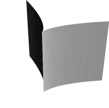
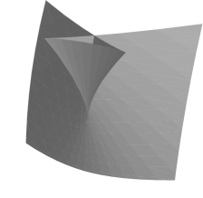
Figure 1. A cuspidal edge and a swallowtail

Proposition 2.19.

Let $f:M^{2}\to{\boldsymbol{R}}^{3}$ be a $C^{\infty}$ wave front. If $f$ has a cuspidal edge (resp. a swallowtail) singular point, then it corresponds to an $A_{2}$-point (resp. an $A_{3}$-point) of the induced metric $d\sigma^{2}(:=df\cdot df)$. Conversely, if a germ of a Kossowski metric at an $A_{2}$-point $($resp. an $A_{3}$-point$)$ is real analytic and $Kd\hat{A}$ does not vanish, then it can be realized as the induced metric of a wave front with cuspidal edges $($resp. a swallowtail$)$.

Proof.

Comparing Definition 2.18 and Fact A.1 in the appendix, we get the first assertion. Finally, we get the second assertion applying Fact 2.17. ∎

Remark 2.20.

If $f$ is not a wave front, singular points of $f$ corresponding to $A_{2}$-points (resp. $A_{3}$-points) of the first fundamental form might not be cuspidal edges (resp. swallowtails). In fact, a cuspidal cross cap $f_{CCR}$ given in the appendix (resp. a $C^{\infty}$ map $f_{2}$ given in [11, Example 1.6]) is a frontal (but not a front) which induces a Kossowski metric with an $A_{2}$-point (resp. an $A_{3}$-point) satisfying $Kd\hat{A}=0$. Kossowski metrics might have singular points other than $A_{2}$ or $A_{3}$ in general (cf. the induced metric of the $C^{\infty}$ map $f_{1}$ given in [11, Example 1.6]).

In [11], the limiting normal curvature $\kappa_{\nu}$ is introduced for non-degenerate singular points of wave fronts, which can be interpreted as the normal curvature of the surface with respect to the singular direction. Moreover, in [11], the cuspidal curvature $\kappa_{c}$ along the cuspidal edge singularities was also defined, and it was also shown that the product $\kappa_{\Pi}:=\kappa_{\nu}\kappa_{c}$ is an intrinsic invariant of cuspidal edges. Isometric deformations of cuspidal edges were discussed in [12] and it was shown that $\kappa_{\nu}$ and $\kappa_{c}$ are both extrinsic invariants. The condition $K\,d\hat{A}\neq 0$ (cf. Fact 2.17) is equivalent to the condition that $\kappa_{\nu}\neq 0$ at the singular points. On the other hand, the singular curvature $\kappa_{s}$ along the cuspidal edge singularities was defined in [14], which is an intrinsic invariant, and played an important role in describing the Gauss-Bonnet type formula for closed wave fronts. From now on, we shall explain these two intrinsic invariants $\kappa_{s}$ and $\kappa_{\Pi}$ of cuspidal edge singularities in terms of Kossowski metrics.

Definition 2.21.

Let $p$ be an $A_{2}$-point of a given Kossowski metric $d\sigma^{2}$. Then an adapted (local) coordinate system $(u,v)$ of $M^{2}$ in the sense of Definition 2.5 is called a strongly adapted coordinate system if the $u$-axis consists of singular points. (By the adaptedness, $\partial_{v}\in\mathcal{N}_{(u,0)}$ holds.)

The existence of an strongly adapted coordinate system at a given $A_{2}$-point can be proven easily. Since the strongly adapted coordinate system satisfies the property in the assumption of Corollary 2.8, the following assertion is proved:

Proposition 2.22.

Let $(u,v)$ be a strongly adapted coordinate system. Then it holds that

(2.15) $$F(u,0)=G(u,0)=E_{v}(u,0)=G_{v}(u,0)=0,$$

where $d\sigma^{2}=E\,du^{2}+2F\,du\,dv+G\,dv^{2}$. Moreover, if another local coordinate system $(\xi,\eta)$ satisfies

(2.16) $$v(\xi,0)=u_{\eta}(\xi,0)=0,\quad u_{\xi}(\xi,0)\neq 0,\quad v_{\eta}(\xi,0)\neq 0,$$

then $(\xi,\eta)$ is also a strongly adapted coordinate system.

Let $p$ be an $A_{2}$-point of a given Kossowski metric $d\sigma^{2}$, and $(u,v)$ a strongly adapted coordinate system centered at $p$. Without loss of generality, we may assume that $\lambda_{v}>0$, where $\lambda$ is a function satisfying (2.9). We set

(2.17) $$\kappa_{s}(u):=\frac{-F_{v}E_{u}+2EF_{uv}-EE_{vv}}{2E^{3/2}\lambda_{v}},$$

which is called the singular curvature at the singular point $(u,0)$, where $d\sigma^{2}=E\,du^{2}+2F\,du\,dv+G\,dv^{2}$. As shown in [14], the singular curvature along cuspidal edges has the same expression as (2.17). So the above definition gives a generalization of singular curvature for $A_{2}$-points of Kossowski metrics. The following assertion holds:

Proposition 2.23.

The value of $\kappa_{s}$ does not depend on a choice of strongly adapted coordinate systems satisfying $\lambda_{v}>0$. In particular, it does not depend on the orientation of the singular curve.

Proof.

We let $(\xi,\eta)$ be another strongly adapted coordinate system. Then it holds that

(2.18) $$\tilde{E} =Eu_{\xi}^{2}+2Fu_{\xi}v_{\xi}+Gv_{\xi}^{2},$$

(2.19) $$\tilde{F} =Eu_{\xi}u_{\eta}+F(u_{\xi}v_{\eta}+u_{\eta}v_{\xi})+Gu_{\xi}u_{\eta},$$

(2.20) $$\tilde{G} =Eu_{\eta}^{2}+2Fu_{\eta}v_{\eta}+Gv_{\eta}^{2},$$

where $d\sigma^{2}=\tilde{E}\,d\xi^{2}+2\tilde{F}\,d\xi\,d\eta+\tilde{G}\,d\eta^{2}$. Using (2.15) and (2.16), we have that

$$\tilde{E} =Eu_{\xi}^{2},\qquad\tilde{E}_{\xi}=u_{\xi}^{3}E_{u}+2Eu_{\xi\xi}u_{\xi},$$

$$\tilde{E}_{\eta\eta} =u_{\xi}^{2}v_{\eta}^{2}E_{vv}+u_{\eta\eta}u_{\xi}^{2}E_{u}+2Eu_{\xi}u_{\xi\eta\eta}+4u_{\xi}v_{\eta}v_{\xi\eta}F_{v},$$

$$\tilde{F}_{\eta} =u_{\eta\eta}u_{\xi}E+u_{\xi}v_{\eta}^{2}F_{v},$$

$$\tilde{F}_{\xi\eta} =u_{\eta\eta}u_{\xi}^{2}E_{u}+u_{\eta\eta}u_{\xi\xi}E+u_{\xi}u_{\xi\eta\eta}E+v_{\eta}^{2}u_{\xi}^{2}F_{uv}+v_{\eta}^{2}u_{\xi\xi}F_{v}+2u_{\xi}v_{\xi\eta}v_{\eta}F_{v}$$

hold along the singular curve. Using these relations, one can see that

$$-\tilde{F}_{\eta}\tilde{E}_{\xi}+2\tilde{E}\tilde{F}_{\xi\eta}-\tilde{E}\tilde{E}_{\eta\eta}=u_{\xi}^{4}v_{\eta}^{2}\left(-F_{v}E_{u}+2EF_{uv}-EE_{vv}\right)$$

holds on the $u$-axis. Since $d\sigma^{2}$ is a frontal metric, there exists a $C^{\infty}$-function $\tilde{\lambda}$ such that $\tilde{E}\tilde{G}-\tilde{F}^{2}=\tilde{\lambda}^{2}$. Since $\tilde{\lambda}=\pm(u_{\xi}v_{\eta}-u_{\eta}v_{\xi})\lambda$, the fact that $\lambda(u,0)=0$ implies that

(2.21) $$\tilde{\lambda}_{\eta}=\pm v^{2}_{\eta}u_{\xi}\lambda_{v}$$

holds on the singular curve. Replacing $(\xi,\eta)$ by $(-\xi,\eta)$ if necessary, we may assume that $u_{\xi}>0$. If we assume $\tilde{\lambda}_{\eta}>0$, then $\tilde{\lambda}_{\eta}=v^{2}_{\eta}u_{\xi}\lambda_{v}$ holds. Using the relation $\tilde{E}^{3/2}=u_{\xi}^{3}E^{3/2}$, one can easily check the coordinate independence of the definition of $\kappa_{s}$. The last assertion follows if we consider the coordinate change $(u,v)\mapsto(-u,v)$ (in this case, $F$ and $u$ change to $-F$ and $-u$, respectively). ∎

Definition 2.24.

A strongly adapted coordinate system $(u,v)$ at an $A_{2}$-point $p$ is said to be normalized if it satisfies the following three conditions:

• $E(u,0)=1$,

• $\lambda_{v}(u,0)=\pm 1$, that is, $G_{vv}(u,0)=2$,

• $F(u,v)=0$,

where $E$, $F$, $G$, $\lambda$ are smooth functions given by $d\sigma^{2}=E\,du^{2}+2\,F\,du\,dv+G\,dv^{2}$ and $EG-F^{2}=\lambda^{2}$.

Proposition 2.25.

Let $p$ be an $A_{2}$-point of a Kossowski metric $d\sigma^{2}$. Then there exists a normalized strongly adapted coordinate system at $p$.

Proof.

We fix a strongly adapted coordinate system $(U;a,b)$ at $p$, and let $d\sigma^{2}=\check{E}\,da^{2}+2\check{F}\,da\,db+\check{G}\,db^{2}$. Then

$$X:=\partial_{a},\qquad Y:=-\check{F}\partial_{a}+\check{E}\partial_{b}$$

are two vector fields on $U$ that are mutually orthogonal. Then by applying the lemma in Page 182 just after Proposition 5.2 in Kobayashi-Nomizu [5], there exists a local coordinate system $(x,y)$ such that $\partial_{x}$ and $\partial_{y}$ are proportional to $X$ and $Y$, respectively, and $y(a,0)=0$ (namely, the singular set is the $x$-axis). Moreover, since $\partial_{b}$ is the null direction on the singular set $\{b=0\}$, $Y$ gives a null vector field along the singular set. Thus $(x,y)$ is a strongly adapted coordinate system. Since $X$, $Y$ are orthogonal, the metric has the expression

$$d\sigma^{2}=\hat{E}\,dx^{2}+\hat{G}\,dy^{2},$$

where $\hat{E}(>0)$ and $\hat{G}$ are smooth functions in $(x,y)$. Consider the coordinate change

$$\xi:=\int_{0}^{x}\sqrt{\hat{E}(t,0)}\,dt,\qquad\eta:=y,$$

which is strongly adapted, and the metric can be expressed by $d\sigma^{2}=\tilde{E}\,d\xi^{2}+\tilde{G}\,d\eta^{2}$ with

$$\tilde{E}(\xi,0)=1.$$

In particular, $\tilde{G}_{\eta\eta}>0$ holds on the $\xi$-axis. In fact, since $d\sigma^{2}$ is frontal, there exists a smooth function $\tilde{\lambda}$ such that $\tilde{\lambda}^{2}=\tilde{E}\tilde{G}$. Since $\tilde{\lambda}=0$ on the singular set $\{\eta=0\}$, non-degeneracy (cf. Definition 2.12) implies $\tilde{\lambda}_{\eta}\neq 0$ on the $\xi$-axis. Differentiating $\tilde{\lambda}^{2}=\tilde{E}\tilde{G}$ twice with respect to $\eta$, we have

$$2\lambda\lambda_{\eta\eta}+2(\lambda_{\eta})^{2}=2\tilde{E}_{\eta}\tilde{G}_{\eta}+\tilde{E}_{\eta\eta}\tilde{G}+\tilde{E}\tilde{G}_{\eta\eta}.$$

Then by Proposition 2.7 and Corollary 2.8, it holds on the $\xi$-axis that

$$\tilde{G}_{\eta\eta}=2(\lambda_{\eta})^{2}>0,$$

and hence $\tilde{G}_{\eta\eta}(\xi,0)>0$. Now we set

$$u:=\xi,\qquad v:=\frac{\eta}{\sqrt[4]{\tilde{G}_{\eta\eta}(\xi,0)/2}},$$

giving a desired normalized strongly adapted coordinate system as follows: By definition, we have the expression $d\sigma^{2}=E\,du^{2}+G\,dv^{2}$. It is obvious that $\partial_{v}$ is perpendicular to $\partial_{u}$. Differentiating (2.20), we get

$$\tilde{G}_{\eta\eta}=G_{vv}v_{\eta}^{4},$$

where we used the facts $u_{\eta}=F_{\eta}=0$ on the $\xi$-axis. So $G_{vv}=2$ holds on the singular curve. Differentiating $\lambda^{2}=EG-F^{2}=EG$ by $v$ twice, and using the fact that $G_{v}(u,0)=0$, we get $\lambda_{v}(u,0)=1$, proving the assertion. ∎

Definition 2.26.

Let $\{(U_{\alpha};u_{\alpha},v_{\alpha},\lambda_{\alpha})\}_{\alpha\in\Lambda}$ be a family of quadruple satisfying (2.12). An adapted coordinate system $(u,v):=(u_{\alpha},v_{\alpha})$ centered at a singular point $p$ is said to be compatible with respect to the co-orientation of $d\sigma^{2}$ if $\partial\lambda_{\alpha}/\partial v_{\alpha}$ is positive at $p$.

Let $(u,v)$ and $(\xi,\eta)$ be two normalized strongly adapted coordinate systems at an $A_{2}$-point $p$. Then the property $\lambda_{v}(u,0)=1$ yields that $v(\xi,0)=0$ and $v_{\eta}(\xi,0)=1$. Hence if the limit

$$\lim_{v\to 0}vK(u,v)$$

exists, it does not depend on a choice of such $(u,v)$ up to $\pm$-ambiguity, where $K$ is the Gaussian curvature of $d\sigma^{2}$. The following assertion holds:

Proposition 2.27.

Let $(U;u,v)$ be a normalized strongly adapted coordinate system at an $A_{2}$-point of a given Kossowski metric $d\sigma^{2}$. Then the limit

$$\tilde{\kappa}_{\Pi}:=\displaystyle\lim_{v\to 0}vK(u,v)$$

exists, whose absolute valued $|\tilde{\kappa}_{\Pi}|$ does not depend on a choice of such $(u,v)$. Moreover, if $d\sigma^{2}$ is co-oriented and $(U;u,v)$ is compatible with respect to the co-orientation of $d\sigma^{2}$, then $\tilde{\kappa}_{\Pi}$ itself is determined without $\pm$-ambiguity.

Proof.

By Theorem 2.15, $K\,\lambda du\wedge dv=K\,d\hat{A}$ is a smooth $2$-from on $M^{2}$, and thus $K\,\lambda$ is a $C^{\infty}$-function on $U$. Since $K\lambda=(vK)(\lambda/v)$, the facts $\lambda(u,0)=0$ and $\lambda_{v}=1$ yield that $\lambda/v$ is a non-vanishing smooth function near the $u$-axis. Thus $vK(u,v)$ is also a smooth function near the $u$-axis, which proves the assertion. ∎

By [11, (2.16)], we get the following assertion, which is a refinement of [11, Theorem 2.17].

Corollary 2.28.

Let $f:M^{2}\to{\boldsymbol{R}}^{3}$ be a wave front, and $p\in M^{2}$ a cuspidal edge singular point of $f$. Then the absolute value of $\tilde{\kappa}_{\Pi}$ at $p$ as an $A_{2}$-point with respect to the first fundamental form of $f$ coincides with that of product curvature $\kappa_{\Pi}$ at $p$ defined in [11].

As an application of the existence of normalized strongly adapted coordinate systems at $A_{2}$-points, we can give the following characterization of Kossowski metrics at singularities:

Proposition 2.29.

Let $p$ be an $A_{2}$-point of a Kossowski metric $d\sigma^{2}$. Then there exists a local coordinate system $(u,v)$ centered at $p$ and smooth function germs $\alpha$, $\beta$ at $p$ so that

(2.22) $$d\sigma^{2}=\bigl{(}1+v^{2}\alpha\bigr{)}du^{2}+v^{2}\bigl{(}1+v\beta\bigr{)}dv^{2}.$$

Conversely, any metrics described as in (2.22) give germs of Kossowski metrics having $A_{2}$-points at the origin.

Proof.

Let $(u,v)$ be a normalized strongly adapted coordinate system at $p$ having the expression $d\sigma^{2}=E\,du^{2}+G\,dv^{2}$. Since $E=1$ holds on the $u$-axis, there exists a $C^{\infty}$-function germ $A$ at $p$ such that $E(u,v)-1=vA(u,v)$. By differentiating it,

$$E_{v}=(E-1)_{v}=vA_{v}+A$$

holds. Since $E_{v}=0$ holds along the $u$-axis, $A=E_{v}-vA_{v}$ also vanishes on the $u$-axis. By Lemma 2.16, we can write $A=v\alpha$, where $\alpha$ is a $C^{\infty}$-function germ at $p$. So we get the expression $E=1+v^{2}\alpha(u,v)$. On the other hand, by using the relations $G=G_{v}=0$, there exists a $C^{\infty}$-function germ $B$ such that $G=v^{2}B(u,v)$. Since $G_{vv}(u,0)=2$, we can write $B-1=v\beta(u,v)$, where $\beta$ is a $C^{\infty}$-function germ, and get the expression

$$G=v^{2}B(u,v)=v^{2}\bigl{(}1+v\beta(u,v)\bigr{)},$$

which proves the first assertion. The second assertion can be proved easily. ∎

Remark 2.30.

Under the expression (2.22) of the Kossowski metric at an $A_{2}$-point, the singular curvature $\kappa_{s}$ and the product curvature $\tilde{\kappa}_{\Pi}$ at $p$ are given by

(2.23) $$\kappa_{s} =-\alpha(u,0),$$

(2.24) $${\tilde{\kappa}}_{\Pi} =\frac{\alpha(u,0)\beta(u,0)-3\alpha_{v}(u,0)}{2}.$$

Using (2.24), we get the following assertion.

Corollary 2.31 (An intrinsic characterization of cuspidal edges).

Let $p$ be a cuspidal edge singular point of a wave front $f:M^{2}\to{\boldsymbol{R}}^{3}$, whose limiting normal curvature $\kappa_{\nu}$ does not vanish at $p$. Then there exists a local coordinate system $(u,v)$ centered at $p$ such that the first fundamental form of $f$ has the expression (2.22). Conversely, if $\alpha,\beta$ are two real analytic function germs, then the metric $d\sigma^{2}$ given by (2.22) can be realized as a first fundamental form of a real analytic wave front in ${\boldsymbol{R}}^{3}$ under the assumption that

(2.25) $$\alpha\beta-3\alpha_{v}\neq 0.$$

Proof.

In [11], it was shown that $\kappa_{\Pi}\neq 0$ is equivalent to the condition $Kd\hat{A}\neq 0$. So Fact 2.17 and (2.24) give the conclusion. ∎

A refinement of Corollary 2.31 is given in [12], where the ambiguity of such a realization is discussed and a normalization theorem of generic cuspidal edges is given by the use of this ambiguity.

3. Gauss-Bonnet formulas for Kossowski metrics

Let $M^{2}$ be an oriented $2$-manifold. A vector bundle $\mathcal{E}$ of rank $2$ with a metric $\left\langle{~{}},{~{}}\right\rangle$ and a metric connection $D$ is called a coherent tangent bundle if there is a bundle homomorphism

$$\psi\colon{}TM^{2}\longrightarrow\mathcal{E}$$

such that

(3.1) $$D_{X}\psi(Y)-D_{Y}\psi(X)=\psi([X,Y])$$

holds for all vector fields $X,Y$ on $M^{2}$ (cf. [15] and [16]).

In this setting, the pull-back of the metric $d\sigma^{2}:=\psi^{*}\left\langle{~{}},{~{}}\right\rangle$ is called the first fundamental form of $\psi$. A point $p\in M^{2}$ is called a singular point (of $\psi$) if $\psi_{p}\colon{}T_{p}M^{2}\to\mathcal{E}_{p}$ is not a bijection, where $\mathcal{E}_{p}$ is the fiber of $\mathcal{E}$ at $p$. The singular points of $\psi$ are the singular points of $d\sigma^{2}$.

The vector bundle $\mathcal{E}$ is called orientable if there exists a smooth non-vanishing skew-symmetric bilinear section $\mu$ of $M^{2}$ into $\mathcal{E}^{*}\wedge\mathcal{E}^{*}$ such that $\mu(e_{1},e_{2})=\pm 1$ for any orthonormal frame $\{e_{1},e_{2}\}$ on $\mathcal{E}$, where $\mathcal{E}^{*}\wedge\mathcal{E}^{*}$ denotes the determinant line bundle of the dual bundle $\mathcal{E}^{*}$. The form $\mu$ is uniquely determined up to $\pm$-ambiguity. An orientation of the coherent tangent bundle $\mathcal{E}$ is a choice of $\mu$. A frame $\{e_{1},e_{2}\}$ is called positive with respect to the orientation $\mu$ if $\mu(e_{1},e_{2})=1$.

Theorem 3.1.

Let $d\sigma^{2}$ be a Kossowski metric defined on a $2$-manifold $M^{2}$ without boundary. Then there exists a coherent tangent bundle

$$\psi:TM^{2}\longrightarrow(\mathcal{E},\left\langle{~{}},{~{}}\right\rangle,D)$$

such that the first fundamental form induced by $\psi$ coincides with $d\sigma^{2}$. Moreover, $\mathcal{E}$ is orientable if $d\sigma^{2}$ is co-orientable.

Proof.

Let $\{(U_{\alpha};u_{\alpha},v_{\alpha})\}_{\alpha\in\Lambda}$ be a covering of $M^{2}$ consisting of local adapted coordinate systems which are compatible with respect to the orientation of $M^{2}$. Since $d\sigma^{2}$ is a Kossowski metric, there exists a $C^{\infty}$-function $\lambda_{\alpha}$ on $U_{\alpha}$ ($\alpha\in\Lambda$) such that

$$E_{\alpha}G_{\alpha}-(F_{\alpha})^{2}=(\lambda_{\alpha})^{2},$$

where $d\sigma^{2}=E_{\alpha}du_{\alpha}^{2}+2F_{\alpha}du_{\alpha}dv_{\alpha}+G_{\alpha}dv^{2}_{\alpha}$ on $U_{\alpha}$.

We fix two indices $\alpha,\beta\in\Lambda$ so that $U_{\alpha}\cap U_{\beta}\neq\emptyset$, and set

$$d\sigma^{2}=E\,du^{2}+2F\,du\,dv+G\,dv^{2}=\tilde{E}\,d\xi^{2}+2\tilde{F}\,d\xi\,d\eta+\tilde{G}\,d\eta^{2},$$

where we set

$$(U;u,v):=(U_{\alpha};u_{\alpha},v_{\alpha}),\qquad(V;\xi,\eta):=(U_{\beta};u_{\beta},v_{\beta})$$

for the sake of simplicity. We now set

$$(\boldsymbol{e}_{1},\boldsymbol{e}_{2}) =(\partial_{u},\partial_{v})\mathcal{T}_{\alpha},\qquad\mathcal{T}_{\alpha}:={\begin{pmatrix}1/\sqrt{E}&-F/(\lambda\sqrt{E})\\ 0&\sqrt{E}/\lambda\end{pmatrix}},$$

$$(\tilde{\boldsymbol{e}}_{1},\tilde{\boldsymbol{e}}_{2}) =(\partial_{\xi},\partial_{\eta})\mathcal{T}_{\beta},\qquad\mathcal{T}_{\beta}:={\begin{pmatrix}1/\sqrt{\tilde{E}}&-\tilde{F}/(\tilde{\lambda}\sqrt{\tilde{E}})\\ 0&\sqrt{\tilde{E}}/\tilde{\lambda}\end{pmatrix}},$$

where $\lambda:=\lambda_{\alpha}$ and $\tilde{\lambda}:=\lambda_{\beta}$ (cf. (2.13)). Then $(\boldsymbol{e}_{1},\boldsymbol{e}_{2})$ and $(\tilde{\boldsymbol{e}}_{1},\tilde{\boldsymbol{e}}_{2})$ are orthonormal frame fields on $U\setminus\Sigma$ and $V\setminus\Sigma$ respectively, where $\Sigma$ denotes the singular set of the metric $d\sigma^{2}$ on $M^{2}$. It holds on $(U\cap V)\setminus\Sigma$ that

(3.2) $$(\tilde{\boldsymbol{e}}_{1},\tilde{\boldsymbol{e}}_{2})=(\boldsymbol{e}_{1},\boldsymbol{e}_{2})\mathcal{T}_{\alpha}^{-1}\mathcal{J}_{\alpha\beta}\mathcal{T}_{\beta},\qquad\mathcal{J}_{\alpha\beta}:={\begin{pmatrix}u_{\xi}&u_{\eta}\\ v_{\xi}&v_{\eta}\end{pmatrix}}.$$

In particular,

(3.3) $$g_{\alpha\beta}:=\mathcal{T}_{\alpha}^{-1}\mathcal{J}_{\alpha\beta}\mathcal{T}_{\beta}$$

can be considered as a matrix valued function defined on $(U\cap V)\setminus\Sigma$ which takes values in the orthogonal group $\operatorname{O}(2)$. Since two local coordinate systems $(u,v)$ and $(\xi,\eta)$ are adapted, (3.3) can be reduced to

$$\sqrt{E\tilde{E}}\,g_{\alpha\beta}=\left(\begin{array}[]{cc}Eu_{\xi}+Fv_{\xi}&-E(\tilde{F}/\tilde{\lambda})u_{\xi}+E\tilde{E}(u_{\eta}/\tilde{\lambda})-F(\tilde{F}/\tilde{\lambda})v_{\xi}+(F/\tilde{\lambda})\tilde{E}v_{\eta}\\ v_{\xi}\lambda&(\tilde{E}v_{\eta}-\tilde{F}v_{\xi})(\lambda/\tilde{\lambda})\\ \end{array}\right).$$

Here, by (2.6) and Lemma 2.16,

$$\tilde{F}/\tilde{\lambda},\quad u_{\eta}/\tilde{\lambda},\quad F/\tilde{\lambda},\quad\lambda/\tilde{\lambda}$$

are smooth functions on $U\cap V$. Since $E\tilde{E}>0$ on $U\cap V$, we can conclude that $g_{\alpha\beta}$ can be extended as a smooth map

$$g_{\alpha\beta}:U_{\alpha}\cap U_{\beta}\to\operatorname{O}(2).$$

Since $g_{\alpha\beta}$ is a transition function of the restriction of vector bundle $TM^{2}$ into $M^{2}\setminus\Sigma$, the co-cycle condition

(3.4) $$g_{\alpha\beta}g_{\beta\gamma}g_{\gamma\alpha}=\operatorname{id}$$

holds on $M^{2}\setminus\Sigma$. By the continuity, (3.4) holds on the whole of $M^{2}$. Thus, there exists a vector bundle $\mathcal{E}$ with inner product $\left\langle{~{}},{~{}}\right\rangle$ whose transition functions are $\{g_{\alpha\beta}\}$, namely, there exist smooth orthonormal frame fields $\Gamma_{\alpha}$ of $\mathcal{E}$ ($\alpha\in\Lambda$) satisfying

(3.5) $$\Gamma_{\beta}=\Gamma_{\alpha}g_{\alpha\beta}\qquad(\alpha,\beta\in\Lambda).$$

By (2.14), we can get a smooth $1$-form $\omega_{\alpha}:=\omega$ on $U_{\alpha}$. Since ${\begin{pmatrix}0&\omega_{\alpha}\\ -\omega_{\alpha}&0\end{pmatrix}}$ is a usual connection form of the Levi-Civita connection of $d\sigma^{2}$, the identity

(3.6) $${\begin{pmatrix}0&\omega_{\beta}\\ -\omega_{\beta}&0\end{pmatrix}}=g_{\alpha\beta}^{-1}(dg_{\alpha\beta})+g_{\alpha\beta}^{-1}{\begin{pmatrix}0&\omega_{\alpha}\\ -\omega_{\alpha}&0\end{pmatrix}}g_{\alpha\beta}$$

holds on $(U\cap V)\setminus\Sigma$. Then by the continuity of $\{\omega_{\alpha}\}$ and $\{g_{\alpha\beta}\}$, (3.6) holds on $U\cap V$. For each $\alpha$, we set

$$D_{w}\hat{e}_{1}:=-\omega_{\alpha}(w)\hat{e}_{2},\qquad D_{w}\hat{e}_{2}:=\omega_{\alpha}(w)\hat{e}_{1}\qquad(w\in TU),$$

where $\Gamma_{\alpha}=(\hat{e}_{1},\hat{e}_{2})$. By (3.6), $D$ gives a globally defined metric connection of $\mathcal{E}$.

We now define a bundle homomorphism $\psi:TM^{2}|_{M^{2}\setminus\Sigma}\to\mathcal{E}|_{M^{2}\setminus\Sigma}$ by

$$\psi(\boldsymbol{e}_{1})=\hat{e}_{1},\qquad\psi(\boldsymbol{e}_{2})=\hat{e}_{2},$$

where $TM^{2}|_{M^{2}\setminus\Sigma}$ (resp. $\mathcal{E}|_{M^{2}\setminus\Sigma}$) is the restriction $TM^{2}$ (resp. $\mathcal{E}$) to $M^{2}\setminus\Sigma$. By (3.2), (3.3) and (3.5), it can be easily checked that the definition of $\psi$ does not depend on the choice of the index $\alpha$. Moreover, the definition of $\psi$ yields that $(\psi(\partial_{u}),\psi(\partial_{v}))=\Gamma_{\alpha}\mathcal{T}_{\alpha}^{-1}$. Since

$$\mathcal{T}^{-1}_{\alpha}={\begin{pmatrix}\sqrt{E}&F/\sqrt{E}\\ 0&\lambda/\sqrt{E}\end{pmatrix}}$$

is a matrix-valued $C^{\infty}$-function on $U=U_{\alpha}$, $\psi$ can be smoothly extended as a bundle homomorphism $\psi:TM^{2}\to\mathcal{E}$. The transition functions $g_{\alpha\beta}$ and the connection forms $\omega_{\alpha}$ are common in two vector bundles $TM^{2}|_{M^{2}\setminus\Sigma}$ and $\mathcal{E}|_{M^{2}\setminus\Sigma}$. Moreover, $D$ can be identified with the Levi-Civita connection of the metric $d\sigma^{2}$ on $M\setminus\Sigma$ by $\psi$, since $\{\omega_{\alpha}\}_{\alpha\in\Lambda}$ consists of the connection forms of the Levi-Civita connection. Hence it satisfies (3.1) on $M^{2}\setminus\Sigma$. Then by the continuity, (3.1) holds on $M^{2}$, which proves $(\mathcal{E},\left\langle{~{}},{~{}}\right\rangle,D)$ is a coherent tangent bundle.

By the definition of $\psi$, $d\sigma^{2}$ is the pull-back metric of $\left\langle{~{}},{~{}}\right\rangle$ by $\psi$ on $M^{2}\setminus\Sigma$, and the continuity of $\psi$ implies that $d\sigma^{2}$ is the first fundamental form of $\psi$ on $M^{2}$. If $d\sigma^{2}$ is co-orientable, one can choose the family $\{\lambda_{\alpha}\}$ so that $\lambda_{\alpha}\lambda_{\beta}$ takes the same sign as $\det(\mathcal{J}_{\alpha\beta})$, which implies that the determinant of $g_{\alpha\beta}$ given by (3.3) is positive. Hence

$$\mu:=\operatorname{sgn}(\lambda_{\alpha})\hat{e}_{1}\wedge\hat{e}_{2}$$

does not depend on the choice of the index $\alpha$, and gives a non-vanishing section of $M^{2}$ into $\mathcal{E}^{*}\wedge\mathcal{E}^{*}$. ∎

As a corollary of Theorem 3.1, we get the following two Gauss-Bonnet formulas:

Proposition 3.2.

Let $d\sigma^{2}$ be a Kossowski metric on a compact orientable $2$-manifold $M^{2}$ without boundary. Suppose that $d\sigma^{2}$ admits at most $A_{2}$ or $A_{3}$-singularities. Then its Gaussian curvature $K$ satisfies

(3.7) $$2\pi\chi(M^{2})=\int_{M^{2}}K\,dA+2\int_{\Sigma}\!\kappa_{s}\,d\tau,$$

where $\Sigma$ denotes the singular set of the metric $d\sigma^{2}$, and $\kappa_{s}$ is the singular curvature defined by (2.17), and $\tau$ is the arclength parameter of the singular curve.

For compact wave fronts in ${\boldsymbol{R}}^{3}$, this formula was shown in Kossowski [7]. (The singular curvature $\kappa_{s}$ is not defined in [7]. Kossowski treated $\kappa_{s}\,d\tau$ as a differential form.)

Proof.

Let $(\mathcal{E},\langle~{},~{}\rangle,D)$ be the coherent tangent bundle induced by the Kossowski metric $d\sigma^{2}$ as in Theorem 3.1. Then, the singular curvature function $\kappa_{s}$ is defined by [15, (1.7)], and one can easily check that it has the expression (2.17) which can be proved by modifying the proof of [14, Proposition 1.8]. Moreover, the proof of [15, Proposition 2.11] implies that $\kappa_{s}\,d\tau$ gives a $C^{\infty}$-form on $1$-dimensional manifold $\Sigma$. Thus (3.7) holds by applying by the second identity of [15, Theorem B]. We remark that the proof of [15, Theorem B] is given under the assumption that $\mathcal{E}$ is orientable. However, taking a double covering of $M^{2}$ if necessary, we may assume that $\mathcal{E}$ is orientable. Since the unsigned area element $dA$ is invariant under the covering transformation, we get the identity without assuming the orientability of $\mathcal{E}$. ∎

Proposition 3.3.

Let $d\sigma^{2}$ be a co-oriented Kossowski metric on a compact oriented $2$-manifold $M^{2}$ without boundary. Suppose that $d\sigma^{2}$ admits at most $A_{2}$ and $A_{3}$-singularities. Then the following identity holds:

(3.8) $$\chi_{\mathcal{E}}:=\frac{1}{2\pi}\int_{M^{2}}K\,d\hat{A}=\chi(M_{+})-\chi(M_{-})+\#S_{+}-\#S_{-},$$

where $\chi_{\mathcal{E}}$ is the Euler characteristic of the oriented coherent tangent vector bundle $(\mathcal{E},\left\langle{~{}},{~{}}\right\rangle,D)$ associated to $d\sigma^{2}$, $M_{+}$ (resp. $M_{-}$) is the subset where $d\hat{A}$ is positively (resp. negatively) proportional to $dA$, and $\#S_{+}$ (resp. $\#S_{-}$) is the number of positive (resp. negative) $A_{3}$-points.

For compact wave fronts in ${\boldsymbol{R}}^{3}$, this formula was shown in Langevin, Levitt and Rosenberg [9].

Proof.

The identity (3.7) holds by applying by the first identity of [15, Theorem B]. ∎

We get the following corollary:

Corollary 3.4.

Let $d\sigma^{2}$ be a co-orientable Kossowski metric on an orientable compact $2$-manifold $M^{2}$ without boundary. Suppose that $d\sigma^{2}$ admits at most $A_{2}$ and $A_{3}$-singularities. Then the number of $A_{3}$-points is even.

4. Whitney metrics and cross caps

Let $U$ be a neighborhood of the origin $o$ in the $uv$-plane ${\boldsymbol{R}}^{2}$. A $C^{\infty}$-map germ $f:(U,o)\to{\boldsymbol{R}}^{3}$ is called a cross cap if there exists a diffeomorphism germ $\varphi$ (resp. $\Phi$) of ${\boldsymbol{R}}^{2}$ (of ${\boldsymbol{R}}^{3}$) such that $\Phi\circ f\circ\varphi(u,v)=(u,uv,v^{2})$. Whitney [19] gave a useful criterion for this singularities. If $(0,0)$ is a cross cap singularity of $f$, then West [18] showed that there exists a local coordinate system $(u,v)$, and a motion $T$ in ${\boldsymbol{R}}^{3}$ such that

(4.1) $$T\circ f(u,v)=\left(u,uv+\sum_{i=3}^{n}\frac{b_{i}}{i!}v^{i},\sum_{r=2}^{n}\sum_{j=0}^{r}\frac{a_{j\,r-j}}{j!(r-j)!}u^{j}v^{r-j}\right)+O(u,v)^{n+1},$$

where $a_{02}\neq 0$ and $O(u,v)^{n+1}$ is a higher order term (cf. [18], see also [2] and [3]). By orientation preserving coordinate changes $(u,v)\mapsto(-u,-v)$ and $(x,y,z)\mapsto(-x,y,-z)$, we may assume that

(4.2) $$a_{02}>0,$$

where $(x,y,z)$ is the usual Cartesian coordinate system of ${\boldsymbol{R}}^{3}$. After this normalization (4.2), one can regard all of the coefficients $a_{jk}$ and $b_{i}$ as invariants of cross caps. An oriented local coordinate system $(u,v)$ giving such a normal form is called the canonical coordinate system of $f$ at the cross cap singularity. In [3], isometric deformations of cross caps are constructed (cf. Figure 2), and it was shown that the coefficients $a_{03}$, $a_{12}$, $b_{3}$ can be changed by such deformations.

Figure 2. An isometric deformation of the standard cross cap.

On the other hand, it was shown in [3] that $a_{02}$, $a_{20}$, $a_{11}$ are all intrinsic invariants. As a refinement of this fact, we will now define a new class of semi-definite metrics called ‘Whitney metrics’  and will reformulate $a_{02},\,\,a_{20},\,\,a_{11}$ as invariants of isolated singularities of such metrics, as follows:

Definition 4.1.

Let $M^{2}$ be a $2$-manifold, and $p$ a singular point of an admissible (positive semi-definite) metric $d\sigma^{2}$ on $M^{2}$ in the sense of Definition 2.3. Let $(u,v)$ be a local coordinate system centered at $p$ and set

$$\delta:=EG-F^{2},$$

where $d\sigma^{2}=E\,du^{2}+2Fdu\,dv+G\,dv^{2}$. If the Hessian

$$\operatorname{Hess}_{u,v}(\delta):=\det{\begin{pmatrix}\delta_{uu}&\delta_{uv}\\ \delta_{uv}&\delta_{vv}\end{pmatrix}}$$

does not vanish at $p$, then $p$ is called an intrinsic cross cap of $d\sigma^{2}$ (cf. Corollary 4.5). Moreover, if $d\sigma^{2}$ admits only intrinsic cross cap singularities, then it is called a Whitney metric.

We fix an intrinsic cross cap $p$ of a given Whitney metric $d\sigma^{2}$ on $M^{2}$. Let $(u,v)$ be a coordinate system as in Definition 4.1. We take another local coordinate system $(\xi,\eta)$ centered at $p$. So it holds that

(4.3) $$\tilde{\delta}=J^{2}\delta\qquad\left(J:=\det{\begin{pmatrix}u_{\xi}&u_{\eta}\\ v_{\xi}&v_{\eta}\end{pmatrix}}\right),$$

where $\tilde{\delta}:=\tilde{E}\tilde{G}-\tilde{F}^{2}$ and $d\sigma^{2}=\tilde{E}\,d\xi^{2}+2\tilde{F}\,d\xi\,d\eta+\tilde{G}\,d\eta^{2}$. Since $\delta\geq 0$, intrinsic cross caps are non-degenerate critical points of $\delta$, and in particular are local minima of $\delta$. Hence it holds that

(4.4) $$\delta_{u}(0,0)=\delta_{v}(0,0)=0,\qquad\text{and}\qquad\delta(u,v)>0\qquad\text{on $V\setminus\{p\}$}$$

for some neighborhood $V$ of $p$. Using these, we have

(4.5) $$\biggl{.}\operatorname{Hess}_{\xi,\eta}(\tilde{\delta})\biggr{|}_{(0,0)}=J(0,0)^{2}\biggl{.}\operatorname{Hess}_{u,v}(\delta)\biggr{|}_{(0,0)},$$

which implies that the definition of intrinsic cross caps is independent of the choice of local coordinate systems.

Example 4.2.

On the $uv$-plane ${\boldsymbol{R}}^{2}$, we set

$$d\sigma^{2}:=e^{\varepsilon(u,v)}\,du^{2}+2F(u,v)\,du\,dv+G(u,v)\,dv^{2}.$$

If the functions $\varepsilon$, $F$ and $G$ satisfy

$$\varepsilon(0,0)=F(0,0)=G(0,0)=0,\quad d\varepsilon(0,0)=dF(0,0)=dG(0,0)=0,$$

$$G(u,v)\geq 0,\qquad\det{\begin{pmatrix}G_{uu}(0,0)&G_{uv}(0,0)\\ G_{uv}(0,0)&G_{vv}(0,0)\end{pmatrix}}\neq 0,$$

then it can be checked that $(0,0)$ is an intrinsic cross cap of $d\sigma^{2}$. Conversely, any Whitney metric has such an expression at its singular point, which is a consequence of the existence of adapted coordinate systems (cf. Definition 4.7 and Proposition 4.8).

Proposition 4.3.

An intrinsic cross cap singular point of $d\sigma^{2}$ is an isolated singular point where the null space (cf. (2.5)) $\mathcal{N}_{p}$ is one dimensional.

In particular, a Kossowski metric cannot be a Whitney metric, since singular points of a Kossowski metric are not isolated (cf. Lemma 2.13).

Proof.

Since non-degenerate critical points of a smooth function are isolated, an intrinsic cross cap is an isolated singular point. Suppose that $\dim\mathcal{N}_{p}=2$. Then it holds that

$$E(0,0)=F(0,0)=G(0,0)=0,$$

where $d\sigma^{2}=E\,du^{2}+2F\,du\,dv+G\,dv^{2}$. Since $d\sigma^{2}$ is positive semi-definite, $E$, $G\geq 0$ hold, and $(0,0)$ is a critical points of the functions $E,F$. Thus we have

$$E_{u}(0,0)=E_{v}(0,0)=G_{u}(0,0)=G_{v}(0,0)=0.$$

Then we get

$$\left.\operatorname{Hess}_{u,v}(\delta)\right|_{(0,0)}=4\det{\begin{pmatrix}-F_{u}(0,0)^{2}&-F_{u}(0,0)F_{v}(0,0)\\ -F_{u}(0,0)F_{v}(0,0)&-F_{v}(0,0)^{2}\end{pmatrix}}=0,$$

which contradicts that $p$ is an intrinsic cross cap. ∎

Proposition 4.4.

Let $p$ be an intrinsic cross cap of a Whitney metric $d\sigma^{2}$, and $(u,v)$ a local coordinate system adjusted at $p$ in the sense of Definition 2.5. Then the identity

$$\delta_{uu}\delta_{vv}-\delta_{uv}^{2}=4E\Delta,\qquad\Delta:=\left.\det{\begin{pmatrix}E&F_{u}&F_{v}\\ F_{u}&G_{uu}/2&G_{uv}/2\\ F_{v}&G_{uv}/2&G_{vv}/2\end{pmatrix}}\right|_{(0,0)}$$

holds at $(u,v)=(0,0)$, where $\delta:=EG-F^{2}$ and $d\sigma^{2}=\,Edu^{2}+2F\,du\,dv+G\,dv^{2}$.

Proof.

Since $p$ is an admissible singular point of $d\sigma^{2}$ and $(u,v)$ is a local coordinate system adjusted at $p$,

$$F(0,0)=G(0,0)=G_{u}(0,0)=G_{v}(0,0)=0$$

hold (cf. Proposition 2.7). Differentiating $\delta:=EG-F^{2}$ twice, we have

$$\delta_{uu}=EG_{uu}-2F_{u}^{2},\quad\delta_{uv}=EG_{uv}-2F_{u}F_{v},\quad\delta_{vv}=EG_{vv}-2F_{v}^{2}$$

at $p=(0,0)$. Then one can get the identity by a straightforward calculation. ∎

As a corollary, we can show the following assertion, which is a reason why we call $p$ an ‘intrinsic cross cap’.

Corollary 4.5.

Let $f:M^{2}\to{\boldsymbol{R}}^{3}$ be a $C^{\infty}$-map and $p$ a cross cap singularity of $f$. Then the first fundamental form $d\sigma^{2}$ of $f$ is an admissible metric, and $p$ is an intrinsic cross cap of $d\sigma^{2}$.

Proof.

By Proposition 2.4, $p$ is an admissible singular point of the metric $d\sigma^{2}$. We take a local coordinate system $(u,v)$ centered at $p$ such that $f_{v}(0,0)=0$, in particular, $(u,v)$ is a local coordinate system adjusted at $p$. By a well-known criterion of cross caps by Whitney [19], the three vectors

$$f_{u}(0,0),\quad f_{uv}(0,0),\quad f_{vv}(0,0)$$

must be linearly independent at $f(p)$. In particular,

(4.6) $${\begin{pmatrix}f_{u}\\ f_{uv}\\ f_{vv}\end{pmatrix}}(f_{u},f_{uv},f_{vv})={\begin{pmatrix}E&F_{u}&F_{v}\\ F_{u}&G_{uu}/2&G_{uv}/2\\ F_{v}&G_{uv}/2&G_{vv}/2\end{pmatrix}}$$

is a regular matrix, where

$$E=f_{u}\cdot f_{u},\quad F=f_{u}\cdot f_{v},\quad G=f_{v}\cdot f_{v}.$$

Taking the determinant of (4.6), the conclusion follows from Proposition 4.4. ∎

The following assertion gives a characterization of the coefficient $a_{02}$ of cross caps in terms of Whitney metrics.

Proposition 4.6.

Let $p\in M^{2}$ be an intrinsic cross cap of a given Whitney metric $d\sigma^{2}$. Let $(u,v)$ be a local coordinate system adjusted at $p$ (cf. Definition 2.5) and set

$$\alpha:=\frac{E(0,0)G_{vv}(0,0)}{2}-F_{v}(0,0)^{2},$$

where $d\sigma^{2}=E\,du^{2}+2F\,du\,dv+G\,dv^{2}$. Then

(4.7) $$\alpha_{02}:=\frac{\sqrt{E(0,0)}\alpha^{3/2}}{\Delta}$$

is a positive value, which does not depend on the choice of local coordinate systems adjusted at $p$ (cf. Definition 2.5). Moreover, $\alpha_{02}$ coincides with the coefficient $a_{02}$ in (4.1) if $d\sigma^{2}$ is induced by the cross cap in ${\boldsymbol{R}}^{3}$.

Proof.

It can be easily checked that $\alpha=\delta_{vv}(0,0)/2$ where $\delta=EG-F^{2}$. Since $\operatorname{Hess}_{u,v}(\delta)\neq 0$, we have that $\alpha>0$. On the other hand, by Proposition 4.4, it holds that

$$4E(0,0)\Delta=\delta_{uu}(0,0)\delta_{vv}(0,0)-\delta_{uv}(0,0)^{2}>0,$$

and we get the inequality $\alpha_{02}>0$.

Let $(\xi,\eta)$ be another local coordinate system adjusted at $p$. We set $\tilde{\delta}=\tilde{E}\tilde{G}-\tilde{F}^{2}$. By (2.7) and (2.6), it holds that

(4.8) $$\tilde{E}(0,0)=E(0,0)u_{\xi}(0,0)^{2}.$$

By (4.3) and (2.6), we have

(4.9) $$\tilde{\delta}(0,0)=\biggl{(}u_{\xi}(0,0)v_{\eta}(0,0)\biggr{)}^{2}\delta(0,0).$$

By (2.6), $\tilde{\delta}_{\eta\eta}(0,0)=\tilde{\delta}_{vv}(0,0)v_{\eta}(0,0)^{2}$ holds. Moreover, since $\delta=\delta_{u}=\delta_{v}=0$ holds at $(0,0)$, we have that

$$\tilde{\delta}_{\eta\eta}(0,0)=\delta_{vv}(0,0)(u_{\xi}(0,0))^{4}(v_{\eta}(0,0))^{6}.$$

Then (4.8) yields

(4.10) $$(\tilde{E}(0,0)\tilde{\delta}_{\eta\eta}(0,0))^{3/2}=(u_{\xi}v_{\eta})^{6}\biggl{(}E(0,0)\delta_{vv}(0,0)\biggr{)}^{3/2}.$$

On the other hand, 4.5, we have

$$\operatorname{Hess}_{\xi,\eta}(\tilde{\delta})(0,0)=(u_{\xi}v_{\eta})^{6}{\operatorname{Hess}}_{u,v}(\delta)(0,0).$$

By this equality and (4.10), we get

(4.11) $$\frac{(\tilde{E}(0,0)\tilde{\delta}_{\eta\eta}(0,0))^{3/2}}{\operatorname{Hess}_{\xi,\eta}(\tilde{\delta})(0,0)}=\frac{(E(0,0)\delta_{vv}(0,0))^{3/2}}{\operatorname{Hess}_{u,v}(\delta)(0,0)},$$

which implies the coordinate invariance of $\alpha_{02}$. Then the last assertion follows from [3, Corollary 8]. ∎

We next give formulations for $a_{20}$ and $a_{11}$ in terms of Whitney metrics.

Definition 4.7.

Let $p$ be a singular point of a Whitney metric. If a local coordinate system $(u,v)$ adjusted at $p$ satisfies

$$E(0,0)=1,\qquad dE(0,0)=dF(0,0)=dG(0,0)=0,$$

then it is called an adapted coordinate system at $p$, where $d\sigma^{2}=E\,du^{2}+2F\,du\,dv+G\,dv^{2}$.

The following assertion can be easily proved.

Proposition 4.8.

There exists an adapted coordinate system at a given intrinsic cross cap. Moreover, if $(u,v)$ and $(\xi,\eta)$ are two adapted coordinate systems at $p$, then

(4.12) $$u_{\xi}(0,0)=\pm 1,\qquad u_{\eta}(0,0)=u_{\xi\xi}(0,0)=u_{\xi\eta}(0,0)=u_{\eta\eta}(0,0)=0$$

hold. Conversely, under the assumption that $(u,v)$ is adapted, a new coordinate system $(\xi,\eta)$ adjusted at $p$ is also an adapted coordinate at $p$ if it satisfies (4.12).

Proof.

Let $(u,v)$ be an adjusted coordinate system centered at $p$, and set

$$u(\xi,\eta)=c_{1}\xi+c_{11}\xi^{2}+c_{12}\xi\eta+c_{22}\eta^{2},\qquad v(\xi,\eta)=\eta$$

for constants $c_{1}$, $c_{11}$, $c_{12}$ and $c_{22}$. Then one can choose these constants such that $(\xi,\eta)$ is adapted, using (2.18), (2.19) and (2.20). The last assertion follows immediately. ∎

Definition 4.9.

An adapted coordinate system $(u,v)$ at an intrinsic cross cap $p\in M^{2}$ is called a West type coordinate system of the second order if there exist two real numbers $\alpha_{20}$ and $\alpha_{11}$ such that

$$E =1+(\alpha_{20})^{2}u^{2}+2\alpha_{11}\alpha_{20}uv+(1+(\alpha_{11})^{2})v^{2}+O(u,v)^{3},$$

$$F =\alpha_{11}\alpha_{20}u^{2}+(1+(\alpha_{11})^{2}+\alpha_{02}\alpha_{20})uv+\alpha_{02}\alpha_{11}v^{2}+O(u,v)^{3},$$

$$G =(1+(\alpha_{11})^{2})u^{2}+2\alpha_{02}\alpha_{11}uv+(\alpha_{02})^{2}v^{2}+O(u,v)^{3},$$

where $d\sigma^{2}=E\,du^{2}+2F\,du\,dv+G\,dv^{2}$ and $\alpha_{02}$ is given by (4.7).

The following assertion can be proved easily, and is the reason why we call $(u,v)$ is of West type:

Proposition 4.10.

A canonical coordinate system at a cross cap singular point is a West type coordinate system of the second order. Moreover, $\alpha_{20}$ and $\alpha_{11}$ coincide with the corresponding coefficients $a_{20}$ and $a_{11}$ in (4.1).

The following assertion holds:

Theorem 4.11.

There exists a West type coordinate system of the second order at each intrinsic cross cap.

To prove the theorem, we prepare several definitions and lemmas:

Definition 4.12.

An adapted coordinate system $(u,v)$ at an intrinsic cross cap $p$ is said to be adjusted in the first-level if $G_{vv}(0,0)=2(\alpha_{02})^{2}$, where $G=d\sigma^{2}(\partial_{v},\partial_{v})$.

By definition, a West type coordinate system of the second order is adjusted in the first-level.

Lemma 4.13.

There exists an adapted coordinate system $(u,v)$ with first-level adjustment at an intrinsic cross cap $p$. Moreover, if an adapted coordinate system $(\xi,\eta)$ at $p$ satisfies

(4.13) $$v_{\eta}(0,0)=\pm 1,$$

then $(\xi,\eta)$ is also an adapted coordinate system adjusted in the first-level.

Proof.

Let $(u,v)$ be an adapted coordinate system at $p$. Then the new coordinate system $(\xi,\eta)$ given by

$$u=\xi,\qquad v=\frac{\sqrt[4]{2}\sqrt{\alpha_{02}}}{\sqrt[4]{G_{vv}(0,0)}}\eta$$

has the desired property. ∎

Remark 4.14.

Let $(u,v)$ be an adapted coordinate system adjusted in the first-level at an intrinsic cross cap $p$. Since $E(0,0)=1$ and $F_{v}(0,0)=0$ by the definition of adaptedness (cf. Definition 4.7), $\alpha$ in Proposition 4.6 satisfies $\alpha=\frac{G_{vv}(0,0)}{2}$. By $G_{vv}(0,0)=2(a_{02})^{2}$, we have $\alpha=(\alpha_{02})^{2}$. So we have

$$\Delta=\frac{\alpha^{3/2}}{\alpha_{02}}=(\alpha_{02})^{2}=\frac{G_{vv}(0,0)}{2}.$$

Definition 4.15.

An adapted coordinate system $(u,v)$ adjusted in the first-level is said to be adjusted in the second-level if

(4.14) $$\det{\begin{pmatrix}F_{uu}-E_{uv}/2&G_{uv}\\ F_{uv}-E_{vv}/2&G_{vv}\end{pmatrix}}=0$$

holds at $(0,0)$, where $d\sigma^{2}=E\,du^{2}+2F\,du\,dv+G\,dv^{2}$.

By Definition 4.9, it can be easily checked that a West type coordinate system of the second order is adjusted in the second-level.

Lemma 4.16.

There exists an adapted coordinate system at an intrinsic cross cap $p$ with second-level adjustment. Moreover, under the assumption that $(u,v)$ is an adapted coordinate system with second-level adjustment, an adapted coordinate system $(\xi,\eta)$ at $p$ is adjusted in the second level if and only if

(4.15) $$v_{\eta}(0,0)=\pm 1,\qquad v_{\xi}(0,0)=0.$$

Proof.

Let $(u,v)$ and $(\xi,\eta)$ be two adapted coordinate systems with first-level adjustment. For the sake of simplicity, we consider the case of $u_{\xi}(0,0)=v_{\eta}(0,0)=1$ in (4.12) and (4.13). Then by (2.6), it holds that

$$\det\begin{pmatrix}\tilde{F}_{\xi\xi}-\tilde{E}_{\xi\eta}/2&\tilde{G}_{\xi\eta}\\ \tilde{F}_{\xi\eta}-\tilde{E}_{\eta\eta}/2&\tilde{G}_{\eta\eta}\end{pmatrix}=\det{\begin{pmatrix}F_{uu}-E_{uv}/2&G_{uv}\\ F_{uv}-E_{vv}/2&G_{vv}\end{pmatrix}}+v_{\xi}\det{\begin{pmatrix}G_{uu}&G_{uv}\\ G_{vu}&G_{vv}\end{pmatrix}}$$

at the origin, where $d\sigma^{2}=\tilde{E}\,d\xi^{2}+2\tilde{F}\,d\xi\,d\eta+\tilde{G}\,d\eta^{2}$. Since $(u,v)$ is adapted, $E=1$ and $F_{u}=F_{v}=0$ at the origin. Then by Proposition 4.4,

(4.16) $$\operatorname{Hess}_{u,v}\delta(0,0)=4\Delta=4\det{\begin{pmatrix}G_{uu}(0,0)&G_{uv}(0,0)\\ G_{vu}(0,0)&G_{vv}(0,0)\end{pmatrix}}\neq 0.$$

Thus, if we set

$$u=\xi,\qquad v=\eta+c\xi,$$

for a suitable constant $c$, such that (4.14) holds at $(0,0)$, then $(u,v)$ is a desired adapted coordinate system with second-level adjustment. ∎

Now, we take an adapted coordinate system $(u,v)$ adjusted in the second-level. By Remark 4.14 and (4.16),

(4.17) $$G_{vv}(0,0)=2(\alpha_{02})^{2},$$

(4.18) $$4(\alpha_{02})^{2}=G_{uu}(0,0)G_{vv}(0,0)-G_{uv}^{2}(0,0)$$

hold. We now define a constant $\alpha_{11}$ so that

(4.19) $$G_{uv}(0,0)=2\alpha_{11}\alpha_{02}.$$

Then (4.17) and (4.18) yield that

(4.20) $$G_{uu}(0,0)=2(1+(\alpha_{11})^{2}).$$

Next, we define a constant $\alpha_{20}$ by

(4.21) $$F_{uv}-\frac{E_{vv}}{2}=\alpha_{20}\alpha_{02}.$$

Then it holds that

$$0 =\det{\begin{pmatrix}F_{uu}-E_{uv}/2&G_{uv}\\ F_{uv}-E_{vv}/2&G_{vv}\end{pmatrix}}$$

$$=\det{\begin{pmatrix}F_{uu}-E_{uv}/2&2\alpha_{11}\alpha_{02}\\ \alpha_{20}\alpha_{02}&2(\alpha_{02})^{2}\end{pmatrix}}=2(\alpha_{02})^{2}\det{\begin{pmatrix}F_{uu}-E_{uv}/2&\alpha_{11}\\ \alpha_{20}&1\end{pmatrix}},$$

and we get

(4.22) $$F_{uu}-\frac{E_{uv}}{2}=\alpha_{11}\alpha_{20}.$$

Theorem 4.17.

The two constants $\alpha_{20}$ and $|\alpha_{11}|$ at each intrinsic cross cap singularity do not depend on the choice of an adapted coordinate system $(u,v)$ with second-level adjustment. Moreover, if $M^{2}$ is oriented, then $\alpha_{11}$ is independent of the choice of oriented adapted coordinate systems with second-level adjustment.

Proof.

The coordinate independence of $\alpha_{20}$ and $|\alpha_{11}|$ are proved by using (2.18), (2.19), (2.20), (4.12), (4.15), (4.19) and (4.21). Let $(\xi,\eta)$ be another adapted coordinate system $(u,v)$ with second-level adjustment. Then it holds that

$$\tilde{G}_{\xi\eta}(0,0)=u_{\xi}(0,0)v_{\eta}(0,0)G_{uv}(0,0).$$

If $M^{2}$ is oriented, then an orientation preserving coordinate change between adapted coordinate systems with second-level adjustment should satisfy

$$u_{\xi}(0,0)v_{\eta}(0,0)=1.$$

Thus $G_{uv}(0,0)$ is independent of such a coordinate change, and the equality (4.19) implies the desired coordinate invariance of $\alpha_{11}$. ∎

Corollary 4.18.

Let $(u,v)$ be an oriented adapted coordinate system with second-level adjustment. If we set

$$u=r\cos\theta,\qquad v=r\sin\theta,$$

then the Gaussian curvature $K$ of $d\sigma^{2}$ satisfies

(4.23) $$\lim_{r\to 0}r^{2}K=\frac{\alpha_{02}(\alpha_{20}\cos^{2}\theta-\alpha_{02}\sin^{2}\theta)}{\left(\cos^{2}\theta+(\alpha_{11}\cos\theta+\alpha_{02}\sin\theta)^{2}\right)^{2}}.$$

Proof.

By (4.17), (4.19), (4.20), (4.21) and (4.22) we can write

$$E =1+e_{20}u^{2}+2e_{11}uv+e_{02}v^{2}+O(u,v)^{3},$$

$$F =\frac{1}{2}(\alpha_{11}\alpha_{20}+e_{11})u^{2}+(e_{02}+\alpha_{02}\alpha_{20})uv+f_{02}v^{2}+O(u,v)^{3},$$

$$G =(1+(\alpha_{11})^{2})u^{2}+2\alpha_{02}\alpha_{11}uv+(\alpha_{02})^{2}v^{2}+O(u,v)^{3},$$

where $e_{20},e_{11},e_{02}$ and $f_{02}$ are constants. Substitute them into the formula (1.3). Then one can directly check that the limit does not depend on the constants $e_{20},e_{11},e_{02}$ and $f_{02}$ and can get (4.23). ∎

Remark 4.19.

The formula (4.23) coincides with [3, (20)], that is, the primary divergent term of the Gaussian curvature of an intrinsic cross cap coincides with that of a cross cap in ${\boldsymbol{R}}^{3}$, since the canonical coordinate system of a cross cap is an adapted coordinate system with second-level adjustment.

Proof of Theorem 4.11.

Let $(u,v)$ be an adapted coordinate system adjusted in the second-level. We define a new local coordinate system $(\xi,\eta)$ by

$$u(\xi,\eta)=\xi+c_{30}\xi^{3}+c_{21}\xi^{2}\eta+c_{12}\xi\eta^{2}+c_{03}\eta^{3},\qquad v(\xi,\eta)=\eta$$

and can adjust the above four coefficients. In fact, $c_{30}$ is adjusted to get $E_{uu}=(\alpha_{20})^{2}$, $c_{21}$ is adjusted for $F_{uu}=2\alpha_{11}\alpha_{20}$, $c_{21}$ is for $F_{uv}=1+(\alpha_{11})^{2}+\alpha_{02}\alpha_{11}$, and $c_{03}$ is for $F_{vv}=2\alpha_{02}\alpha_{11}$. Then $E_{uu}$ and $E_{uv}$ are determined by (4.21) and (4.22). ∎

By the existence of a West type coordinate system, we get the following assertion:

Corollary 4.20.

The two invariants $a_{20}$ and $a_{11}$ of cross caps in ${\boldsymbol{R}}^{3}$ can be extended as corresponding invariants $\alpha_{20}$ and $\alpha_{11}$ for intrinsic cross caps, respectively.

Remark 4.21.

Let $(0,0)$ be an intrinsic cross cap singularity of the metric $d\sigma^{2}=Edu^{2}+2Fdudv+Gdv^{2}$ on an oriented coordinate neighborhood $(U;u,v)$. We set

$$dA:=\sqrt{EG-F^{2}}du\wedge dv.$$

By (4.23), $KdA$ gives a smooth 2-form with respect to the polar coordinate system $(r,\theta)$, where $u=r\cos\theta$ and $v=r\sin\theta$. Thus, the integral $\int_{U}KdA$ is well-defined.

5. Gauss-Bonnet formula for Whitney metrics

At the end of this paper, we shall prove the following Gauss-Bonnet type formula for Whitney metrics:

Theorem 5.1.

Let $M^{2}$ be a compact oriented manifold without boundary, and $d\sigma^{2}$ a Whitney metric in $M^{2}$. Then its Gaussian curvature $K$ satisfies

$$\frac{1}{2\pi}\int_{M^{2}}KdA=\chi(M^{2}),$$

that is, there is no defect at intrinsic cross cap singularities for the Gauss-Bonnet formula.

For compact surfaces which admit only cross cap singularities in ${\boldsymbol{R}}^{3}$, the corresponding formula was shown in Kuiper [6].

Proof.

We fix a singular point $p$ of $d\sigma^{2}$, and take an oriented West type coordinate system of the second order $(U;u,v)$ at $p$. Using the formula (4.23), one can see that $K\,dA$ is a smooth $2$-form on $U$. We set

$$D(r):=\{(u,v)\in U\,;\,u^{2}+v^{2}\leq r^{2}\}$$

and

$$D_{+}(r,\varepsilon):=D(r)\cap\{v\geq\varepsilon\},\qquad D_{-}(r,\varepsilon):=D(r)\cap\{v\leq-\varepsilon\},$$

where $\varepsilon$ is a sufficiently small positive constant. Then we have that

(5.1) $$\int_{D(r)}K\,dA=\lim_{\varepsilon\to 0}\int_{D_{+}(r,\varepsilon)}K\,dA+\lim_{\varepsilon\to 0}\int_{D_{-}(r,\varepsilon)}K\,dA.$$

Moreover, the classical Gauss-Bonnet formula yields that

(5.2) $$\int_{D_{\pm}(r,\varepsilon)}K\,dA=\int_{\partial D_{\pm}(r,\varepsilon)}\kappa_{g}\,ds+\pi,$$

and so

$$\int_{D(r)}KdA=2\pi+\lim_{\varepsilon\to 0}\int_{\partial D_{+}(r,\varepsilon)}\kappa_{g}\,ds+\lim_{\varepsilon\to 0}\int_{\partial D_{-}(r,\varepsilon)}\kappa_{g}\,ds$$

holds. We set

$$L_{+}(\varepsilon):=\partial D_{+}(r,\varepsilon)\setminus\partial D(r),\qquad L_{-}(\varepsilon):=\partial D_{-}(r,\varepsilon)\setminus\partial D(r).$$

Then they are line segments parallel to the $u$-axis. Moreover, we may assume that the orientation of $L_{+}(\varepsilon)$ is the same as that of the $u$-axis, and the orientation of $L_{-}(\varepsilon)$ is opposite that of $L_{+}(\varepsilon)$. These orientations are compatible with respect to the anti-clockwise orientations of $\partial D_{\pm}(r)$. We now compute the geodesic curvature of $L_{+}(\varepsilon)$ for each fixed sufficiently small $\varepsilon(>0)$:

$$\kappa_{g}\,ds=\frac{\langle\nabla_{u}\dot{\gamma}^{\varepsilon}(u),\boldsymbol{n}(u,\varepsilon)\rangle du}{|\dot{\gamma}^{\varepsilon}(u)|^{2}}=\frac{\Gamma(\partial_{u},\partial_{u},\boldsymbol{n})du}{|\dot{\gamma}^{\varepsilon}(u)|^{2}},$$

where $\gamma^{\varepsilon}(u):=(u,\varepsilon)$ ($|u|<\sqrt{r^{2}-\varepsilon^{2}}$) and $\boldsymbol{n}(u,\varepsilon)$ is the co-normal vector field along $\gamma^{\varepsilon}$. If we set $d\sigma^{2}=E\,du^{2}+2F\,du\,dv+G\,dv^{2}$, we have

$$\boldsymbol{n}(u,\varepsilon)=\frac{-F\partial_{u}+E\partial_{v}}{\sqrt{E(EG-F^{2})}}$$

and by a straightforward calculation, we have

$$\left\langle{\nabla_{u}\dot{\gamma}^{\varepsilon}(u)},{\boldsymbol{n}(u,\varepsilon)}\right\rangle=\frac{E(2F_{u}-E_{v})-E_{u}F}{2\sqrt{E(EG-F^{2})}}.$$

Since $|\dot{\gamma}^{\varepsilon}(u)|^{2}=E(u,\varepsilon)$, we get

$$\kappa_{g}\,ds=\frac{(E(2F_{u}-E_{v})-E_{u}F)du}{2\sqrt{E^{3}(EG-F^{2})}}.$$

By setting, $u=r\cos\theta$, $v=r\sin\theta$, it holds that

$$\kappa_{g}\,ds=\frac{du}{E^{3/2}}\frac{\alpha_{20}(\alpha_{11}\cos\theta+\alpha_{02}\sin\theta)+rO_{1}(r,\theta)}{\sqrt{(1+(\alpha_{11})^{2})\cos^{2}\theta+2\alpha_{02}\alpha_{11}\cos\theta\sin\theta+(\alpha_{02})^{2}\sin^{2}\theta+rO_{2}(r,\theta)}},$$

where $O_{i}(r,\theta)$ ($i=1,2$) are $C^{\infty}$-functions of $r,\theta$. Since the light-hand side is bounded, we can show that

(5.3) $$\lim_{\varepsilon\to 0}\int_{L_{+}(\varepsilon)}\kappa_{g}\,ds=\int_{L_{+}(0)}\kappa_{g}\,ds.$$

Since $\lim_{\varepsilon\to 0}\kappa_{g}\,ds$ is not continuous at $u=0$ as a $1$-form on the $u$-axis, the integrals should be taken to be Lebesgue integrals. Similarly, we have

(5.4) $$\lim_{\varepsilon\to 0}\int_{L_{-}(\varepsilon)}\kappa_{g}\,ds=\int_{L_{-}(0)}\kappa_{g}ds=-\int_{L_{+}(0)}\kappa_{g}\,ds.$$

Thus, we get

(5.5) $$\int_{D(r)}K\,dA=2\pi+\int_{\partial D}\kappa_{g}\,ds.$$

The relations (5.5), (5.1) and (5.2) imply the assertion. ∎

It is well-known that even numbers of cross caps appear in closed surfaces in ${\boldsymbol{R}}^{3}$ which admit only cross cap singularities. In the previous section, we have shown that the number of $A_{3}$-points is even under the assumption that the Kossowski metric is co-orientable. However, the above Gauss-Bonnet formula does not give any such restriction of the number of intrinsic cross caps. In fact, one can construct a Whitney metric on a torus having only one intrinsic cross cap as follows: The $C^{\infty}$-map $f(u,v)=(u,uv,v^{2})$ has a cross cap singularity at the origin, and its first fundamental form is given by

$$ds^{2}:=\left(1+v^{2}\right)\,du^{2}+2\,uv\,du\,dv+\left(u^{2}+4v^{2}\right)\,dv^{2}.$$

Let $\rho:{\boldsymbol{R}}\to[0,1]$ be a $C^{\infty}$-function such that $\rho(t)=1$ for $|t|\leq 1/4$ and $\rho(t)=0$ for $|t|\geq 3/4$. We set

$$d\sigma^{2}:=\rho(2r)ds^{2}+(1-\rho(2r))(du^{2}+dv^{2})\qquad\left(r:=\sqrt{u^{2}+v^{2}}\right).$$

Then $d\sigma^{2}$ has a singular point only on $(0,0)$, and is a Whitney metric having an intrinsic cross cap at $(0,0)$, which is defined on the square-shaped closed domain $\overline{D}:=\{(u,v)\in{\boldsymbol{R}}^{2}\,;\,-1\leq u,v\leq 1\}$. Identifying each of two pairs of the parallel edges of the boundary of $\bar{D}$, the metric $d\sigma^{2}$ can be considered as a Whitney metric on the square torus having only one cross cap singularity.

Appendix A Wave fronts, cuspidal edges and swallowtails

Let $M^{2}$ be a $2$-manifold and $f:M^{2}\to{\boldsymbol{R}}^{3}$ a $C^{\infty}$-map. A point $p\in M^{2}$ is called regular if $f$ is an immersion on a sufficiently small neighborhood of $p$, and is called singular if it is not regular. A $C^{\infty}$-map $f:M^{2}\to{\boldsymbol{R}}^{3}$ is called a frontal if for each $p\in M^{2}$ there exists a unit normal vector field $\nu$ along $f$ defined on a neighborhood $U_{p}$ of $p$. By parallel displacements in ${\boldsymbol{R}}^{3}$, $\nu$ can be considered as a map $\nu:U_{p}\to S^{2}$. In this case, $\nu$ is called the Gauss map of the frontal $f$. Moreover, if the map

$$L:=(f,\nu):U_{p}\to{\boldsymbol{R}}^{3}\times S^{2}$$

gives an immersion for each $p\in M^{2}$, $f$ is called a front or a wave front. Using the canonical inner product, we identify the unit tangent bundle $T_{1}{\boldsymbol{R}}^{3}={\boldsymbol{R}}^{3}\times S^{2}$ with the unit cotangent bundle $T_{1}^{*}{\boldsymbol{R}}^{3}$, which has the canonical contact structure. When $f$ is a front, $L$ gives a Legendrian immersion.

Let $f:M^{2}\to{\boldsymbol{R}}^{3}$ be a frontal. Then $f$ is called co-orientable if there exists a smooth unit normal vector field $\nu$ globally defined on $M^{2}$. We fix a singular point $p\in M^{2}$ of $f$ and take a local coordinate system $(U_{p};u,v)$ of $p$. The function on $U_{p}$ defined by

$$\lambda:=\det(f_{u},f_{v},\nu)$$

is called a signed area density function. The set $\{(u,v)\in U_{p}\,;\,\lambda(u,v)=0\}$ coincides with the singular set of $f$ on $U_{p}$. A singular point $p$ is called non-degenerate if the exterior derivative $d\lambda$ of $\lambda$ does not vanish at $p$. (This definition does not depend on the choice of local coordinate systems at $p$.) On a neighborhood of a non-degenerate singular point, the singular set consists of a regular curve $\gamma(t)$, called the singular curve. The tangential direction of the singular curve is called the singular direction, and the direction of the kernel of $df$ is called the null direction. Let $\eta(t)$ be the smooth (non-vanishing) vector field along the singular curve which gives the null direction.

Here, we give examples: A singular point is called a cuspidal edge or a swallowtail if the corresponding germ of $C^{\infty}$-map is right-left equivalent to that of $C^{\infty}$-map

(1) $$f_{C}(u,v):=(u^{2},u^{3},v)\quad\text{or}\quad f_{S}(u,v):=(3u^{4}+u^{2}v,4u^{3}+2uv,v)$$

at $(u,v)=(0,0)$, respectively. Here, two $C^{\infty}$-maps $f\colon{}(U,p)\to{\boldsymbol{R}}^{3}$ and $g\colon{}(V,q)\to{\boldsymbol{R}}^{3}$ are right-left equivalent at the points $p\in U$ and $q\in V$ if there exists a local diffeomorphism $\varphi$ of ${\boldsymbol{R}}^{2}$ with $\varphi(p)=q$ and a local diffeomorphism $\Psi$ of ${\boldsymbol{R}}^{3}$ with $\Psi(f(p))=g(q)$ such that $g=\Psi\circ f\circ\varphi^{-1}$. It can be easily checked that both of $f_{C}$ and $f_{S}$ are fronts whose singular sets are all non-degenerate. These two types of singular points characterize the generic singularities of wave fronts. The singular curve of $f_{C}$ is the $v$-axis and the null direction is the $u$-direction. The singular curve of $f_{S}$ is the parabola $6u^{2}+v=0$ and the null direction is the $u$-direction. The following criteria are known:

Fact A.1 ([8]).

Let $f:M^{2}\to{\boldsymbol{R}}^{3}$ be a front. Let $p\in M^{2}$ be a non-degenerate singular point, and $\gamma(t)$ the singular curve of $f$ such that $\gamma(0)=p$. Then

1. $p$ is a cuspidal edge if and only if the null direction $\eta(0)$ is transversal to the singular direction $\dot{\gamma}(0)$,

2. $p$ is a swallowtail if and only if the null direction $\eta(0)$ is proportional to the singular direction $\dot{\gamma}(0)$, and satisfies

   $$\left.\frac{d}{dt}\right|_{t=0}\det(\dot{\gamma}(t),\eta(t))\neq 0.$$

A cuspidal cross cap is a singular point which is right-left equivalent to the $C^{\infty}$-map

(A.1) $$f_{CCR}(u,v):=(u,v^{2},uv^{3}),$$

which is not a front but a frontal with unit normal vector field

$$\nu_{CCR}:=\frac{1}{\sqrt{4+9u^{2}v^{2}+4v^{6}}}(-2v^{3},-3uv,2).$$

Using (1) of Fact A.1, one can easily check that all of singular points of $f_{CCR}$ except for the origin consist of cuspidal edges.

References

• [1] T. Fukui, J. J. Nuño-Ballesteros, Isolated rounding and flattenings of submanifolds in Euclidean spaces, Tohoku Math. J. 57 (2005), 469–503.
• [2] T. Fukui and M. Hasegawa, Fronts of Whitney umbrella–a differential geometric approach via blowing up– Journal of Singularities, 4 (2012), 35-67.
• [3] M. Hasegawa, A. Honda, K. Naokawa, M. Umehara, and K. Yamada, Intrinsic invariants of cross caps, Selecta Mathematica, 20 (2014), 769-785.
• [4] N.H. Kuiper, Stable surfaces in Euclidean three space, Math. Scand 36, (1975) 83–96.
• [5] S. Kobayashi, K. Nomizu, Foundations of Differential Geometry, Volume I, Wiley-Interscience (1964).
• [6] M. Kossowski, Realizing a singular first fundamental form as a nonimmersed surface in Euclidean 3-space , J. Geom. 81 (2004) 101–113.
• [7] M. Kossowski, The Boy-Gauss-Bonnet theorems for $C^{\infty}$-singular surfaces with limiting tangent bundle, Ann. Global Anal. Geom. 21 (2002), 19–29.
• [8] M. Kokubu, W. Rossman, K. Saji, M. Umehara and K. Yamada, Singularities of flat fronts in hyperbolic space, Pacific J. Math., 221 (2005), 303–351.
• [9] R. Langevin, G. Levitt, and H. Rosenberg, Classes d’homotopie de surfaces avec rebroussements et queues d’aronde dans $R^{3}$, Canad. J. Math. 47 (1995), 544–572.
• [10] L. F. Martins and K. Saji, Geometric invariants of cuspidal edges, preprint.
• [11] L. F. Martins, K. Saji, M. Umehara, and K. Yamada, Behavior of Gaussian curvature around non-degenerate singular points on wave fronts, preprint, arXiv:1308.2136.
• [12] K. Naokawa, M. Umehara and K. Yamada, Isometric deformations of cuspidal edges, to appear in Tohoku Math. J., arXiv:1408.4243.
• [13] M. Spivak, A comprehensive Introduction to Differential Geometry V, Publish or Perish Inc. Houston, Texas, 1999.
• [14] K. Saji, M. Umehara, and K. Yamada, The geometry of fronts, Ann. of Math., 169 (2009), 491–529.
• [15] K. Saji, M. Umehara and K. Yamada, Behavior of corank one singular points on wave fronts, Kyushu Journal of Mathematics 62 (2008), 259–280.
• [16] K. Saji, M. Umehara and K. Yamada, Coherent tangent bundles and Gauss-Bonnet formulas for wave fronts, Journal of Geometric Analysis 22 (2012) 383-409, DOI 10.1007/s12220-010-9193-5.
• [17] S. Shiba and M. Umehara, The behavior of curvature functions at cusps and inflection points, Diff. Geom. Appl., 30 (2012), 285–299.
• [18] J. West, The differential geometry of the cross-cap, Ph. D. thesis, Liverpool Univ. 1995.
• [19] H. Whitney, The general type of singularity of a set of $2n-1$ smooth functions of $n$ variables, Duke Math. J. 10 (1943), 161–172.