ON THE BLOCKAGE PROBLEM AND THE NON-ANALYTICITY OF THE CURRENT FOR THE PARALLEL TASEP ON A RING

Abstract

The Totally Asymmetric Simple Exclusion Process (TASEP) is an important example of a particle system driven by an irreversible Markov chain. In this paper we give a simple yet rigorous derivation of the chain stationary measure in the case of parallel updating rule. In this parallel framework we then consider the blockage problem (aka slow bond problem). We find the exact expression of the current for an arbitrary blockage intensity $\varepsilon$ in the case of the so-called rule-184 cellular automaton, i.e. a parallel TASEP where at each step all particles free-to-move are actually moved. Finally, we investigate through numerical experiments the conjecture that for parallel updates other than rule-184 the current may be non-analytic in the blockage intensity around the value $\varepsilon=0$.

keywords: Parallel tasep; Blockage Problem; Current

msc2010: 60J10, 37B15, 60K30

1   Introduction

The Totally Asymmetric Simple Exclusion Process (TASEP) is one of the more popular example of discrete particle system driven by a Markov irreversible dynamics [11, 12]. In finite space the system can be defined either on a discrete segment $\Lambda=\{1,2,\ldots,2L\}$ or on a discrete circle by imposing periodic boundary condition to $\Lambda$. A configuration $\sigma\in\{0,1\}^{\Lambda}$ can be viewed as a set of particles living in $\Lambda$. According to this map, $\sigma_{i}=1$ means that the $i$th site is occupied by a particle, whereas if $\sigma_{i}=0$ then the $i$th site is a hole, i. e. it is an empty site.

TASEP may be formulated either as a serial or a parallel dynamics. The serial TASEP chooses an occupied site $i$ uniformly at random; if the right-neighbouring site, i. e. site $i+1$, is a hole then the selected particle jumps to the $(i+1)$th site; conversely the $(i+1)$th site is occupied by another particle, then the configuration does not change and a new iteration starts over. The parallel TASEP selects instead all the particles having an unoccupied right-neighbouring site, but those actually advancing to the empty site are chosen according to a binomial rule, i. e. each particle actually advances with an independent probability $p$. Both serial and parallel dynamics are clearly irreversible.

Despite its simplicity, the serial TASEP exhibits many interesting features. For example, the stationary measure is uniform on a discrete circle since the transition matrix is doubly Markov. On the finite segment the stationary state depends on the probability of a particle entering or exiting the system through the left and right extremes of the segment, respectively (see [4, 20]). In this case the system exhibits a non-trivial behaviour.

The study of TASEP typically focuses on the current, defined as the probability that, under stationary conditions, the $i$th site is a particle and the $(i+1)$th is a hole. This quantity is important because it measures the tendency of the system to exhibit congestion, i. e. the tendency to form long sequences of clustered particles that are not free to move. Remarkably, the current does not depend on $i$ and can be exactly computed for both the serial TASEP defined on the segment and on the discrete circle. In particular, on the discrete circle the current depends only on the number of particles in the system and it is maximum (and equal to $\nicefrac{{1}}{{4}}$ in the limit of $L\to\infty$) when the system is half-filled, i. e. when $L$ particles lie on the circle $\Lambda=\{1,2,...,2L\}$.

Parallel TASEP was first studied on a ring in [15] as a collective dynamics for freeway traffic. The model was extended in [19] to the case of particles performing jumps of length corresponding to their velocity. In the case of jumps limited to next-neighbouring sites (velocity 1), the authors derived through a mean-field approximation the steady-state distribution of the model. However, their derivation is quite involved, requiring to prove that the first order mean-field approximation remains valid at all higher orders. Parallel TASEP on a ring with inhomogeneous jump-rates is studied in [6], where the stationary distribution of the model is given in a form equivalent to [19]. Ref. [18] gives a review of parallel TASEP on a ring with a focus on traffic applications. More recently, the steady-state of a parallel TASEP on a ring where particles can jump one or two sites ahead has been characterised as a scalar-pair factorised and a matrix-product state [22].

Exact solution to parallel TASEP with open boundary conditions is given both in [3] and [7] in terms of a matrix product. An alternative, combinatorial expression in term of Catalan numbers can be found in [5]. Parallel TASEP has been investigated also via Bethe Ansatz imposing both open and periodic boundary. The results obtained so far comprehend the expression of the evolute measure of the model at every time [16, 17, 13].

All formulations of the stationary distribution of the parallel TASEP (both with open and periodic boundary conditions) are considered quite involved in [21], where the author studies parallel TASEP with open boundaries in terms of Motzkin paths. In this respect, our work offers a significant contribution, for it frames the steady state of parallel TASEP in a simple yet fruitful formulation.

A very natural question in the study of the irreversible system is whether the effect of small perturbations in the dynamics has local effects, as in the case of reversible system far from critical points, or global effects. In the case of the TASEP this question has been investigated by imposing the so-called blockage (see [9, 8]), that is to say, in a defined point (say, without loss of generality, in the point $2L$ of the circle) the probability to jump to the empty site $1$ is reduced by a factor $1-\varepsilon$ with $\varepsilon>0$. In terms of freeway traffic, blockage is a synonym for bottleneck and its effects are typically studied by a simulative approach; one of the first studies of this kind is about the so-called rule-184 cellular automaton [23], which is nothing else than a parallel TASEP with deterministic updates, i. e. a parallel TASEP with probability $p=1$.

Answering the question about global effects on the system here simply reduces to the evaluation of the current; if a blockage in a single point influences the value of the current then its effects are obviously global. For a long time it has been unclear whether the presence of a blockage of intensity $\varepsilon$ had global effects for all $\varepsilon>0$. It is conjectured in [2] that the current decreases, for small $\varepsilon$, with a non-analytic dependence on $\varepsilon$. Numerical evaluation of the current may suggest also the existence of a critical value $\varepsilon_{c}>0$ such that the current does not change for $\varepsilon<\varepsilon_{c}$. Only very recently it has been proved [1] that for $\Lambda=\mathbb{Z}$ and continuous time, it is $\varepsilon_{c}=0$. However, the conjecture about the non-analyticity of the current around $\varepsilon=0$ still remains unproved.

In this paper we study the parallel TASEP dynamics, where at each step each particle followed by an empty site has a finite probability $p$ to jump. We show that this model has similar features with respect to the serial TASEP; in particular, considering the blockage problem, we see numerically that for $p<1$ the behaviour of the current is very similar to the standard TASEP case, because for small $\varepsilon$ the current suggests a non-analytic dependence on $\varepsilon$ around $\varepsilon=0$. On the other hand, for $p=1$, we prove that the system with blockage is exactly solvable, and that the current is analytic as a function of $0\leq\varepsilon\leq 1$. Regarding the existence of a critical value $\varepsilon_{c}$, it is likely that the very same argument of [1] may be extended to the case of the discrete circle for both serial and parallel dynamics. We hence expect that, except for the case $p=1$, where the current as a function of $\varepsilon$ has a finite first derivative, the current is non-analytic around $\varepsilon=0$ for all $p<1$.

The paper is organised as follows: in Section 2 we define our parallel irreversible dynamics on the circle, and we compute its stationary distribution. The computation of the stationary measure is quite simple, being based on the idea of dynamical reversibility. In Section 3 we explicitly compute the current of parallel TASEP making use of the exact expression of the stationary measure, and we find with relative ease the expression already known in the literature. In Section 4 we investigate the blockage problem for the parallel TASEP, and we solve it in the particular case of $p=1$, that is to say, the 184-rule with a blockage of intensity $\varepsilon$ in a single site. The stochasticity of the resulting process sits in this case only in the blockage, since in all the other sites the dynamics is deterministic. Finally, in Section 5 we present some numerical simulations and discuss a conjecture inspired by [2] on the non-analyticity of the current around $\varepsilon=0$.

2   The parallel TASEP

In this paper we study the parallel TASEP on a discrete circle, i.e. on the set $\Lambda=\{1,2,...,2L\}$ with periodic boundary conditions. A configuration $\sigma$ is any element of the set $\{0,1\}^{\Lambda}$, which can be though of as a $|\Lambda|$-dimensional vector; the $i$th component of the vector is $\sigma_{i}$. We say that $i$th site is a particle whenever $\sigma_{i}=1$, while the site is a hole if $\sigma_{i}=0$. We allow for negative indexing of the configuration $\sigma$ under the agreement that $\sigma_{-i}=\sigma_{2L-i+1}$

A particle in site $i$ is said to be free to move whenever the site $i+1$ is a hole. Particles move clockwise by exchanging position with the neighbouring hole. In other words, moving a particle means replacing the couple $\sigma_{i}=1,\sigma_{i+1}=0$ with $\sigma_{i}=0,\sigma_{i+1}=1$. As a consequence, holes move counterclockwise. The symbols $\bullet$ and $\times$ are used as convenient shorthands for particles and holes, respectively. Using this notation, the process of moving a particle can be sketched as $\bullet\times\to\times\bullet$.

Each configuration $\sigma$ can be decomposed into particle trains, i. e. maximal sequences of particles lying in adjacent sites. The engine of a train is the element of the sequence with highest index possible; conversely, the caboose is the element with lowest index. Engines are the only particles that can move across a single iteration of the dynamics. Whenever an engine is moved, it may either form a new train of length 1 ($\bullet\bullet\times\times\to\bullet\times\bullet\times$) or become the caboose of another train ($\bullet\bullet\times\bullet\to\bullet\times\bullet\bullet$).

Given a configuration $\sigma$, let $m(\sigma)=\sum_{i=1}^{2L}\sigma_{i}$ be the number of particles living in $\Lambda$. In what follows we assume that $m(\sigma)\leq L$. We indicate by $l(\sigma)\leq m(\sigma)$ the number of engines (or trains) in the configuration $\sigma$.

A transition from the configuration $\sigma$ to the configuration $\tau$ is weighed according to the following rule:

$$w(\sigma,\tau)=\begin{cases}\omega^{n}&\text{if }\tau\text{ can be reached by moving }n\text{ particles in }\sigma,\\ 0&\text{otherwise},\end{cases}$$ (1)

where $\omega>0$ is a positive parameter measuring the tendency of a free particle to move. The resulting transition probabilities are

$$P(\sigma,\tau)=\frac{w(\sigma,\tau)}{w(\sigma)}\,,$$ (2)

where

$$w(\sigma)=\sum_{\tau}w(\sigma,\tau)=\sum_{k=0}^{l(\sigma)}{l(\sigma)\choose k}\omega^{k}=(1+\omega)^{l(\sigma)}.$$ (3)

The dynamics clearly conserves the number of particles in $\Lambda$, i. e. $m(\sigma)=m(\tau)=m$.

For small values of $\omega$ (e. g. $\omega=O(\nicefrac{{1}}{{L}})$), the parallel TASEP is similar to a serial dynamics. For finite values of $\omega$, the dynamics is truly parallel, in the sense that each free-to-move particle advances to the empty neighbouring site with independent probability $p=\nicefrac{{\omega}}{{1+\omega}}$. In the limit of $\omega\to\infty$, $p=1$ and all the free particles simultaneously move at each step (rule-184 cellular automata).

The Markov chain (2) is manifestly irreversible. However, it is still possible to compute the stationary distribution of the chain with relative ease as the chain satisfies the global balance principle [10]

$$\sum_{\tau}w(\sigma,\tau)=\sum_{\tau^{\prime}}w(\tau^{\prime},\sigma)\,.$$ (4)

Equation (4) is fulfilled simply because the final configurations $\tau$ at the left hand side of (4) can be mapped one-to-one onto the initial configurations $\tau^{\prime}$ at the right hand side in such a way that $w(\sigma,\tau)=w(\tau^{\prime},\sigma)$. More precisely, let $\tau$ be the configuration obtained from $\sigma$ by advancing the engine of some particle trains to the empty neighbouring sites; similarly, let $\tau^{\prime}$ the configuration obtained from $\sigma$ by detaching the caboose of the very same set of particle trains; clearly, $w(\sigma,\tau)=w(\tau^{\prime},\sigma)$.

Equation (4) is known in the literature also by the name of dynamical reversibility and guarantees that the stationary measure of the chain is $\pi(\sigma)=\nicefrac{{w(\sigma)}}{{W}}$, where $W=\sum_{\sigma}w(\sigma)$. In fact,

$$\sum_{\sigma}\pi(\sigma)P(\sigma,\tau)=\sum_{\sigma}\frac{w(\sigma)}{W}\frac{w(\sigma,\tau)}{w(\sigma)} =\sum_{\sigma}\frac{w(\sigma,\tau)}{W}$$

$$=\sum_{\sigma}\frac{w(\tau,\sigma)}{W}=\frac{w(\tau)}{W}=\pi(\tau)\,.$$ (5)

Using (3), the stationary measure is

$$\pi(\sigma)=\frac{(1+\omega)^{l(\sigma)}}{W}\,.$$ (6)

Remark 1.

When $\omega\to 0$, $\pi(\sigma)$ tends to the uniform value $\nicefrac{{1}}{{{2L\choose m(\sigma)}}}$. In the limit of $\omega\to\infty$, $\pi(\sigma)$ tends instead to be uniform on all the configurations such that $l(\sigma)=m(\sigma)$ because in this regime $W=O(\omega^{m(\sigma)})$, so other configurations have a weight that is smaller by at least a factor $\nicefrac{{1}}{{1+\omega}}$.

3   Current for the half-filled TASEP

As mentioned in Section 1, the value of the current $J$ in the serial TASEP is the quantity

$$J^{\text{\tiny SRL}}=\lim_{\Lambda\to\infty}\pi^{\text{\tiny SRL}}(\sigma_{i}=1,\sigma_{i+1}=0)\,,$$ (7)

where $\pi^{\text{\tiny SRL}}$ is the stationary distribution of the serial model and $i\in\Lambda$. The event $\{\sigma_{i}=1,\sigma_{i+1}=0\}$ does not actually depend on the site $i$ but only on the number of particles $m$. Therefore, an equivalent formulation for $J^{\text{\tiny SRL}}$ is the following:

$$J^{\text{\tiny SRL}}=\lim_{L\to\infty}\frac{\mathbb{E}_{\pi^{\text{\tiny SRL}}}[l(\sigma)]}{2L}\,,$$ (8)

where $\mathbb{E}_{\pi^{\text{\tiny SRL}}}[\cdot]$ denotes expectation with respect to $\pi^{\text{\tiny SRL}}$.

In what follows, we consider the half-filled case $m=L$, i.e. the number of particles is exactly half the sites. Then, for the serial TASEP,

$$J^{\text{\tiny SRL}}=\pi^{\text{\tiny SRL}}(\sigma_{i}=1,\sigma_{i+1}=0)\simeq\pi^{\text{\tiny SRL}}(\sigma_{i}=1)\pi^{\text{\tiny SRL}}(\sigma_{i+1}=0)=\nicefrac{{1}}{{4}}$$

since the stationary probability $\pi^{\text{\tiny SRL}}$ is uniform, and therefore the probability to have the configuration $\sigma_{i}=1,\sigma_{i+1}=0$ tends, for large $\Lambda$, to the product of the probabilities to have $\sigma_{i}=1$ and ${\sigma_{i+1}=0}$ (and they both equal $\nicefrac{{1}}{{2}}$).

In this section we focus on the current $J$ in the parallel TASEP. Analogously to (7)-(8), let us define the current as

$$J=\pi(\sigma_{i}=1,\sigma_{i+1}=0)=\lim_{L\to\infty}\frac{\mathbb{E}_{\pi}[l(\sigma)]}{2L}\,,$$ (9)

where $\mathbb{E}_{\pi}[\cdot]$ denotes expectation with respect to $\pi$. The following result holds:

lemma 1 For the parallel TASEP (2), the current $J$ satisfies

$$J=\frac{1}{2}\ \frac{\sqrt{1+\omega}}{1+\sqrt{1+\omega}}\,.$$ (10)

Proof.

Let us start by recasting $J$ as

$$J=\lim_{L\to\infty}\frac{1}{2L}\ \frac{\sum_{\sigma}l(\sigma)(1+\omega)^{l(\sigma)}}{\sum_{\sigma}(1+\omega)^{l(\sigma)}}=\lim_{L\to\infty}\frac{1}{2L}\ \frac{\sum_{l=1}^{L}l\ n(l)(1+\omega)^{l}}{\sum_{l=1}^{L}n(l)(1+\omega)^{l}}\,,$$ (11)

where $n(l)$ is the number of configurations $\sigma$ having $l(\sigma)=l$ particles free to move. Next, a formula for $n(l)$ is obtained as follows: first, we count the number of ways for dividing $L$ particles in $l$ distinct trains (and $L$ holes in $l$ trains); suppose that the first train of particles has length $l_{1}$, then we count all the ways for the site $i=1$ to fall within the first particle-train; at this stage a configuration is uniquely determined by the alternate sequence of particle and hole trains; it may also happen that the site $i=1$ falls within a hole train, and this is accounted for by multiplying everything by $2$.

Since $L$ objects can be divided in $l$ ordered groups in ${L-1\choose l-1}$ ways,

$$n(l)=2\sum_{l_{1}=1}^{L-l+1}l_{1}{L-l_{1}-1\choose l-2}{L-1\choose l-1}\,.$$ (12)

Substituting (12) into (11) yields

$$J=\lim_{L\to\infty}\frac{1}{2L}\ \frac{\sum_{l=1}^{L}\sum_{l_{1}=1}^{L-l+1}l_{1}{L-l_{1}-1\choose l-2}{L-1\choose l-1}\ l\ (1+\omega)^{l}}{\sum_{l=1}^{L}\sum_{l_{1}=1}^{L-l+1}l_{1}{L-l_{1}-1\choose l-2}{L-1\choose l-1}(1+\omega)^{l}}\,.$$ (13)

In order to evaluate (13), let us write $l=\alpha L$, $l_{1}=\alpha_{1}L$ and use the leading order approximation

$${n\choose\alpha n}\approx e^{nI(\alpha)}\,,$$ (14)

where $I(\alpha)=-\alpha\ln\alpha-(1-\alpha)\ln(1-\alpha)$. Then,

$$J=\lim_{L\to\infty}\frac{1}{2L}\ L\frac{\int_{0}^{1}d\alpha\int_{0}^{1-\alpha}d\alpha_{1}\ \alpha\,\alpha_{1}\,e^{L\left((1-\alpha_{1})I(\frac{\alpha}{1-\alpha_{1}})+I(\alpha)+\alpha\ln(1+\omega)\right)}}{\int_{0}^{1}d\alpha\int_{0}^{1-\alpha}d\alpha_{1}\,\alpha_{1}\,e^{L\left((1-\alpha_{1})I(\frac{\alpha}{1-\alpha_{1}})+I(\alpha)+\alpha\ln(1+\omega)\right)}}\,.$$ (15)

Let us define

$$f(\alpha,\alpha_{1})=(1-\alpha_{1})I\left(\frac{\alpha}{1-\alpha_{1}}\right)+I(\alpha)+\alpha\ln(1+w)\,.$$

Then, by the saddle-point method,

$$J=\lim_{L\to\infty}\left[\frac{1}{2}\bar{\alpha}+O\left(\frac{1}{L}\right)\right]\,,$$

where $\bar{\alpha}$ is the value of $\alpha$ that maximises $f(\alpha,\alpha_{1})$. Since $f(\alpha,\alpha_{1})$ is a decreasing function of $\alpha_{1}$, the choice $\alpha_{1}=0$ yields

$$\bar{\alpha}=\frac{\sqrt{1+\omega}}{1+\sqrt{1+\omega}}\qquad\text{and}\qquad J=\frac{1}{2}\ \frac{\sqrt{1+\omega}}{1+\sqrt{1+\omega}}\,.$$ (16)

∎

Remark 2.

For $\omega=O(\nicefrac{{1}}{{L}})$, the parallel TASEP is a nearly serial dynamics and, as expected, $J=\nicefrac{{1}}{{4}}$. Moreover, $J$ is an increasing function of $\omega$ and $J=\nicefrac{{1}}{{2}}$ in the limit of $\omega\rightarrow\infty$.

4   Blockage problem for the rule-184 cellular automata

We have mentioned in Section 1 that a very interesting and difficult aspect in the study of serial TASEP is the so-called blockage problem, which is defined as follows for the serial dynamics (see [2] and references therein). At each step a particle is chosen uniformly at random and, if free to move, it is moved to the next site with probability $1$ unless it occupies the site $2L$, in which case it is moved with probability $1-\varepsilon$. An explicit expression for the current is not yet known either for serial nor parallel TASEP.

Very recently, the current $J$ in parallel TASEP was shown in [1] to be strictly less than the maximum value, i.e. $\nicefrac{{1}}{{4}}$, for each $\varepsilon>0$. However, numerical evidences strongly suggest that the current stays very close to its maximum value up to some finite value of $\varepsilon$, see Section 5 below. Therefore, it may be that the current $J$ as a function of $\varepsilon$ behaves as a very high-order polynomial around the value $\varepsilon=0$, or that $J$ has an essential singularity in $\varepsilon=0$ as conjectured in [2].

In this section we study the blockage problem through the parallel TASEP (1)-(3) modified in the following way:

$$w_{\varepsilon}(\sigma,\tau)=\begin{cases}\omega^{n}(1-\varepsilon\mathds{1}_{\{\sigma_{2L}=1,\tau_{2L}=0\}})&\text{if }\tau\text{ can be reached by moving }\\ &n\text{ particles in }\sigma,\\ 0&\text{otherwise},\end{cases}$$ (17)

where $\varepsilon\in(0,1)$ and $\mathds{1}_{\{\cdot\}}$ is the usual indicator function. Weights (17) are identical to (1) save for they penalise by a factor $(1-\varepsilon)$ the transitions $\bullet|\times\to\times|\bullet$ across the blockage, here represented by the symbol $|\,$. Let TASEP with blockage be defined by the following transition probabilities:

$$P_{\varepsilon}(\sigma,\tau)=\frac{w_{\varepsilon}(\sigma,\tau)}{w_{\varepsilon}(\sigma)}\,,$$ (18)

where

$$w_{\varepsilon}(\sigma)=\sum_{\tau}w_{\varepsilon}(\sigma,\tau)\,.$$ (19)

Due to the presence of the blockage, the global balance principle (4) is no longer satisfied by the chain, and finding the stationary measure becomes extremely difficult. However, we will describe the current for finite values of $\omega$ in Section 5 through numerical experiments. Apparently, the blockage problem for parallel TASEP is similar to the serial case: the current seems to be almost constant until $\varepsilon$ reaches a critical value, which is a decreasing function of $\omega$. The possibility of rigorously proving any result about this behaviour seems nevertheless to be as hard as for the serial dynamics.

A happy exception is the regime $\omega\to\infty$, i.e. the rule-184 cellular automata, where all free particles move with probability $p=1$ except the particle at site $2L$, if any, which moves with probability $1-\varepsilon$. This case is easily solvable due to the circumstance that the dynamics preserves the so-called particle-hole symmetry, defined next.

Definition 1.

A configuration $\sigma$ such that $\sigma_{i}=1-\sigma_{-i}$ for each $i=1,2,\ldots,2L$ is said to be particle-hole symmetric (abbrev. ph-symmetric). The set of particle-hole symmetric configurations is denoted by $PH$.

The next result states that in the limit of $\omega\to\infty$ the parallel TASEP with blockage preserves the particle-hole symmetry.

lemma 2 Consider the transition probabilities

$$P_{\varepsilon,\infty}(\sigma,\tau)=\lim_{\omega\to\infty}P_{\varepsilon}(\sigma,\tau)\,.$$ (20)

For each $\varepsilon\in[0,1)$ and for each $\sigma\in PH$, if $P_{\varepsilon,\infty}(\sigma,\tau)>0$ then $\tau\in PH$.

Proof.

Let us fix a site $i\in\{2,3,\ldots,L\}$ and start considering the case $\sigma_{i}=1$. Due to the ph-symmetry, if $\sigma_{i}$ is an engine then also $\sigma_{-i-1}$ is an engine; since in the regime $\omega\to\infty$ the engines move with probability $1$, the sites $i$ and $-i-1$ will become holes, i.e. $\tau_{i}=\tau_{-i-1}=0$, while the sites $i+1$ and $-i$ will be occupied by a particle, i.e. $\tau_{i+1}=\tau_{-i}=1$. Conversely, if $\sigma_{i}$ is not an engine then it must be $\sigma_{i+1}=1$, and so $\sigma_{-i}=\sigma_{-i-1}=0$; therefore, site $i$ will keep being occupied, while site $-i$ will continue being empty, that is to say, $\tau_{i}=1$ and $\tau_{-i}=0$. The case $\sigma_{i}=0$ is completely analogous, but we have to distinguish between site $i$ being or not being the caboose of a hole train. We still have to check what happens across the blockage. The following four configurations are possible:

$$\text{1.}\;\times\times|\bullet\bullet;\quad\text{2.}\;\times\bullet|\times\bullet;\quad\text{3.}\;\bullet\times|\bullet\times;\quad\text{4.}\;\bullet\bullet|\times\times.$$

In the first case site $1$ remains occupied and site $2L$ empty, then $\tau_{1}=1$ and $\tau_{-1}=0$; in the third case site $1$ becomes empty and site $2L$ occupied, then $\tau_{1}=0$ and $\tau_{-1}=1$. Conversely, in the second and fourth case site $1$ becomes occupied and site $2L$ empty with probability $1-\varepsilon$, i.e. $\tau_{1}=1$ and $\tau_{-1}=0$, or with probability $\varepsilon$ the blockage acts on the particle at site $2L$, which remains occupied, i.e. $\tau_{1}=0$ and $\tau_{-1}=1$. ∎

The following two lemmas identify the set of recurrent states of the Markov chain $P_{\varepsilon,\infty}(\sigma,\tau)$.

lemma 3 All states $\sigma\not\in PH$ are transient for the Markov chain $P_{\varepsilon,\infty}(\sigma,\tau)$.

Proof.

Key to the proof is the following observation: for all initial configurations, there exists a finite probability $p>\varepsilon^{2L}$ for the system to be after $2L$ steps in the configuration $\sigma_{\text{queue}}$ such that $\sigma_{i}=0$ for $i=1,2,...,L$ and $\sigma_{i}=1$ for $i=L+1,L+2,...,2L$. Indeed, if the blockage stops the passage of particles for $2L$ times in a row, then the system will surely reach the configuration $\sigma_{\text{queue}}$, which is a state obviously ph-symmetric. Hence, starting from any initial state $\sigma\not\in PH$, there is a finite probability that the system arrives in a symmetric state after $2L$ steps, and in virtue of Lemma 4 it will never visit again $\sigma$. ∎

The next Lemma is motivated by the following easy yet important

Remark 3.

Let us imagine that after some time the system reaches a ph-symmetric configuration such that all particles in $\{1,2,...,L\}$ are free to move, then the particles will be free to move in that half of the circle at any subsequent time. This happens because all the particles in $\{1,2,...,L-1\}$ can never reach the preceding particle (they all move at each step with probability $1$) and if $\sigma_{L}=1$ then $\sigma_{-L}=\sigma_{L+1}=0$, so that the presence of a particle at site $L$ cannot form a queue behind itself.

Definition 2.

We will call $\Omega_{\infty}$ the set of configurations $\sigma\in PH$ such that all the particles in $\{1,2,...,L\}$ are free to move.

lemma 4 For the Markov chain $P_{\varepsilon,\infty}(\sigma,\tau)$ all the states $\sigma\not\in\Omega_{\infty}$ are transient.

Proof.

The proof is analogous to that of Lemma 4. For any starting configuration $\sigma\not\in\Omega_{\infty}$, the system has a finite probability to reach the configuration $\sigma_{\text{queue}}$ in $2L$ steps, and $\sigma_{\text{queue}}\in\Omega_{\infty}$. The thesis then follows from Remark 3. ∎

A direct consequence of Lemma 4 is that the stationary probability $\pi_{\varepsilon,\infty}$ of the Markov chain $P_{\varepsilon,\infty}(\sigma,\tau)$ is supported on $\Omega_{\infty}$, where the latter is manifestly ergodic.

Let $J_{\varepsilon,\infty}=\lim_{L\to\infty}\pi_{\varepsilon,\infty}(\sigma_{i}=1,\sigma_{i+1}=0)$ be the current of parallel TASEP in the regime of $\omega\to\infty$ under the action of a blockage $\varepsilon$, and let $r(\sigma)$ be the number of particles that lie in first half of the circle, i.e. sites $\{1,2,...,L\}$; those particles are free to move by Lemma 4. It is quite obvious that the number of particles free to move in sites $\{L+1,L+2,...,2L\}$ is again $r(\sigma)$ by the ph-symmetry. Then, analogously to what we have done in (9), we can compute $J_{\varepsilon,\infty}$ as

$$J_{\varepsilon,\infty}=\lim_{L\to\infty}\frac{R}{L}\,,$$ (21)

where $R=\mathbb{E}_{\pi_{\varepsilon,\infty}}(r)$ is the expected value of $r(\sigma)$ with respect to the stationary measure $\pi_{\varepsilon,\infty}$.

We are now ready to prove the fundamental result of this section.

proposition 5 The current $J_{\varepsilon,\infty}$ of the Markov chain $P_{\varepsilon,\infty}(\sigma,\tau)$ is

$$J_{\varepsilon,\infty}=\frac{1-\varepsilon}{2-\varepsilon}\,.$$ (22)

Key to the proof of Proposition 4 is the following

Remark 4.

Starting from a state $\sigma\in\Omega_{\infty}$, the first $L$ sites loose any memory of the initial configuration after $L$ steps of the dynamics because the particles are free to move in the first half of the ring. Because of the ph-symmetry, $L$ steps are sufficient also for the second half of the ring to loose any memory of the initial configuration. In other words, let $\sigma_{t}$ be the configuration of the chain after $t$ steps and let $\zeta_{\infty}$ be the hitting time of the set $\Omega_{\infty}$, i.e. $\zeta_{\infty}=\min\{t\geq 0\text{ such that }\sigma_{t}\in\Omega_{\infty}\}$. Then, $\zeta_{\infty}+L$ is a strong stationary time fo rthe chain.

Proof of Proposition 4.

The first part of the proof is the computation of the stationary measure of the chain. We can imagine that, at each step in which $\sigma_{2L}=1$, the blockage is driven by a binary random variable, which can be green, giving at the next step $\tau_{2L}=0$, or red, giving at the next step $\tau_{2L}=1$. Due to the symmetry, we can say that the probability of each state can be written in terms of a sequence of green and red lights. In particular, when the particle has passed the blockage, and therefore $\sigma_{2L}=0,\sigma_{1}=1$, we know that in the next step we will have for sure $\tau_{1}=0,\tau_{2}=1$. By symmetry, this means that we have now a particle in the site $2L$. Hence the next generation of a particle in the set $\{1,2,...,L\}$ is due only to the values of the red light.

Let us first consider the set of states $\sigma\in\Omega_{\infty}$ such that $\sigma_{1}=0$. Then, if site $i$ is occupied then site $i-1$ is a hole with probability $1$. In other words, each particle occupies two sites and so the probability to have a configuration $\sigma$ with $r$ particles lying in $\{1,2,...,L\}$ is

$$\pi_{\varepsilon,\infty}(\sigma)=(1-\varepsilon)^{r}\varepsilon^{L-2r}.$$ (23)

Conversely, if $\sigma_{1}=1$ then the exponents appearing in (23) may increase or decrease by a unit at most. This correction is negligible in the thermodynamic limit, thus we will use (23) to compute the current according to (21). For large $L$,

$$R\approx\frac{\sum_{r=1}^{L/2}r{L-r\choose r}(1-\varepsilon)^{r}\varepsilon^{L-2r}}{\sum_{r=1}^{L/2}{L-r\choose r}(1-\varepsilon)^{r}\varepsilon^{L-2r}},$$ (24)

and we can again evaluate the expression simply by using the approximation in (14) and the saddle-point method. Let us call $x=\frac{r}{L}$ and recast (24) as

$$R\approx L\frac{\int_{0}^{L/2}dx\,x\,e^{L((1-2x)\ln\varepsilon+x\ln(1-\varepsilon)-x\ln\frac{x}{1-x}-(1-2x)\ln\frac{1-2x}{1-x})}}{\int_{0}^{L/2}dx\,e^{L((1-2x)\ln\varepsilon+x\ln(1-\varepsilon)-x\ln\frac{x}{1-x}-(1-2x)\ln\frac{1-2x}{1-x})}}\,.$$ (25)

In the limit of $L\to\infty$,

$$J_{\varepsilon,\infty}=\lim_{L\to\infty}\frac{R}{L}=\bar{x}\,,$$

where $\bar{x}=\frac{1-\varepsilon}{2-\varepsilon}$ is the value of $x$ that maximises

$$f(x)=(1-2x)\ln\varepsilon+x\ln(1-\varepsilon)-x\ln\frac{x}{1-x}-(1-2x)\ln\frac{1-2x}{1-x}\,.$$

∎

Remark 5.

Despite its simplicity, this computation proves, in this completely parallel context, that a very small perturbation of the transition probabilities in a single site extends its effect over all the volume, without any fading. Indeed, the uniform density of the particles in the set $\{1,2,...,L\}$ is $\frac{1-\varepsilon}{2-\varepsilon}$ while in the set $\{L+1,L+2,...,2L\}$ the uniform density is $\frac{1}{2-\varepsilon}$.

5   Numerical results

In this final section we present a series of numerical evidences obtained in a half-filled parallel TASEP with blockage probability $\varepsilon$ acting on the site $2L$ of a ring lattice of $1000$ sites ($L=500$). In particular, we numerically evaluate the current the current, $J(p,\varepsilon)$, and the particle density around site $x$, $\rho(x,p,\varepsilon)$, as functions of both the probability $p=\nicefrac{{\omega}}{{(1+\omega)}}$ of an engine moving to the next site and the blockage intensity $\varepsilon$. The current is computed according to (9), while density (see Section 5.2 below) is computed at points $x\in\{1,2,...,\nicefrac{{2L}}{{10}}\}$ as follows:

$$\rho(x,p,\varepsilon)=\frac{1}{10}\left[\sum_{i=10x}^{10x+9}\sigma_{i}\right].$$

The problem of rigorously evaluating the mixing time of parallel TASEP is not studied in this paper. However, the argument leading to the evaluation of the stationary measure in the case $p=1$ shows that the system reaches the stationary distribution after a time proportional to $L$.

In the general case $p<1$ we run the dynamics for a time

$$T=2\ \frac{L}{p}\leavevmode\nobreak\ log(L)\,.$$

We are not aware of an estimate of the mixing time for the standard TASEP. In the case of the symmetric exclusion process on the circle Morris proved that $T=L^{2}\log L$ (see [14]), and this corresponds in our case to the choice $p=\nicefrac{{1}}{{2L}}$.

Our numerical experiments are particularly focused on two facts:

1. We know from [2] that in serial TASEP the current remains very close to the limit value without blockage. We also know that for the explicitly solvable blockage system discussed in Section 4, i.e. $p=1$ or, equivalently, $\omega\to\infty$, the current has a decrease that is proportional to $\varepsilon$ near the value $\varepsilon=0$. We want to check numerically if the supposed non-analyticity of $J$ around $\varepsilon=0$ is a particular feature of the single spin-flip dynamic, or if it survives to the parallel case. The following figures clearly show that the second scenario seems the one to be true, at least from a numerical point of view.

2. We want to see if the density is an increasing function of the site $x$ when the current decreases, or if the presence of the blockage implies simply a queueing of particles close to it; the solvable model with $p=1$, i.e. $\omega\to\infty$, exhibits the latter behaviour.

5.1   Current

The measure of the current $J$ is simply made by counting the average number of the particles free to move during the evolution of the system and weighing such value with the total volume of the system $2L$.

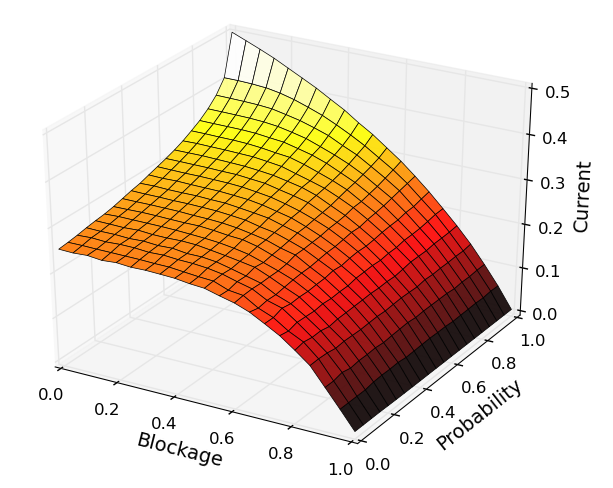
Figure 1: Current in parallel TASEP as function of the probability $p=\nicefrac{{\omega}}{{(1+\omega)}}$ and the blockage intensity $\varepsilon$.

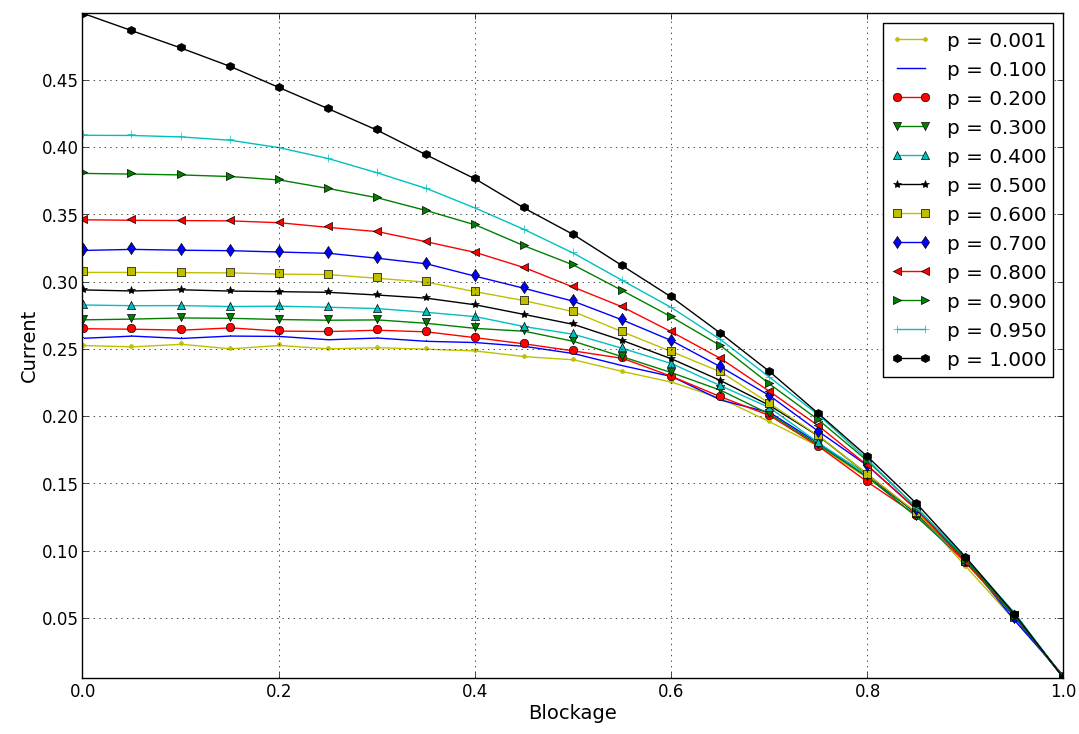
Figure 2: Profile curves of the current in the parallel TASEP for different values of the probability $p=\nicefrac{{\omega}}{{(1+\omega)}}$.

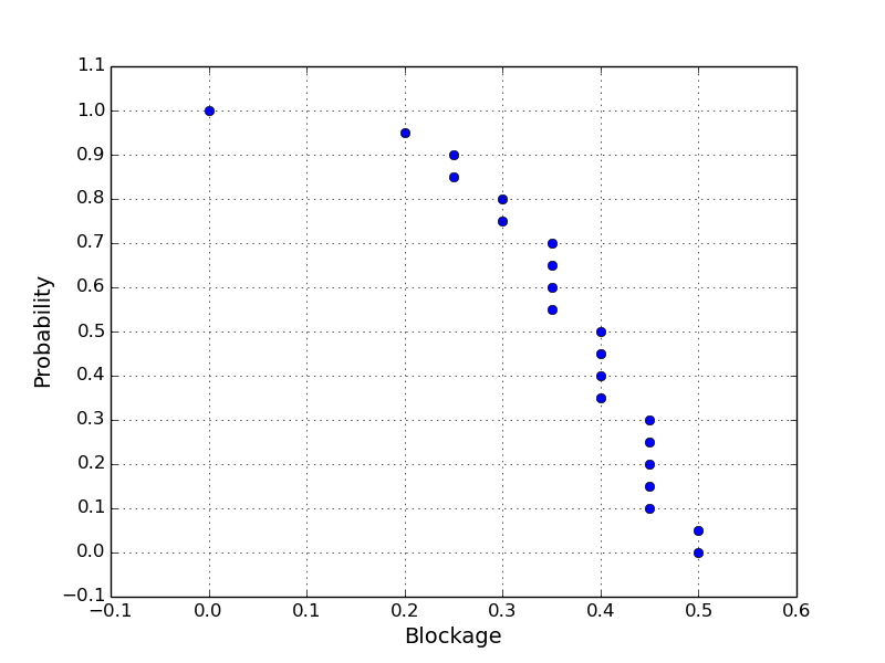
Figure 3: Threshold values of $\varepsilon$ for a $1\%$ deviation from the no-blockage current.

Figure 1 shows the surface obtained interpolating 441 measures of $J$ with every combination of the parameters $\frac{1}{2L}\leq p\leq 1$ and $0\leq\varepsilon\leq 1$, both with increments of $\nicefrac{{25}}{{L}}=0.05$. The figure clearly shows an excellent fit with the currents computed in Lemma 3 and in Proposition 4.

Figure 2 presents the behaviour of the current for $\nicefrac{{1}}{{2L}}\leq p\leq 1$ with increments of $\nicefrac{{25}}{{L}}=0.05$, plotting the side projection of the 3D graph from Figure 1. It clearly appears that except in the case $p=1$, i.e. $\omega\to\infty$, where the current decrease with a finite slope for all $\varepsilon>0$, the decrease of $J$ starts only after a certain value of the blockage. In this respect, the conjectured non-analytical behaviour of the serial TASEP, to which the parallel TASEP corresponds in the regime $p=O(\nicefrac{{1}}{{L}})$, seems to be conserved for all the probabilities except $p=1$.

Figure 3 plots the threshold values of $\varepsilon$ for which the current deviates more than the $1\%$ from its initial value in the absence of blockage. This gives an indication of the shape of the region in which the current remains nearly constant from a numerical point of view, having however $\varepsilon>0$. The description of this behaviour could be investigated after we had achieved a better understanding of the stationary measure in presence of blockage (see open questions below).

5.2   Density

Simulations can be also used to obtain insights about the typical particle distribution over the ring. In order to obtain this characterisation, we have coarse-grained the particles on segments of length 10, in order to obtain the density $\rho$ defined above. The density diagrams below describe the density of segments of the configuration, assigning a darker colour to the more dense segment.

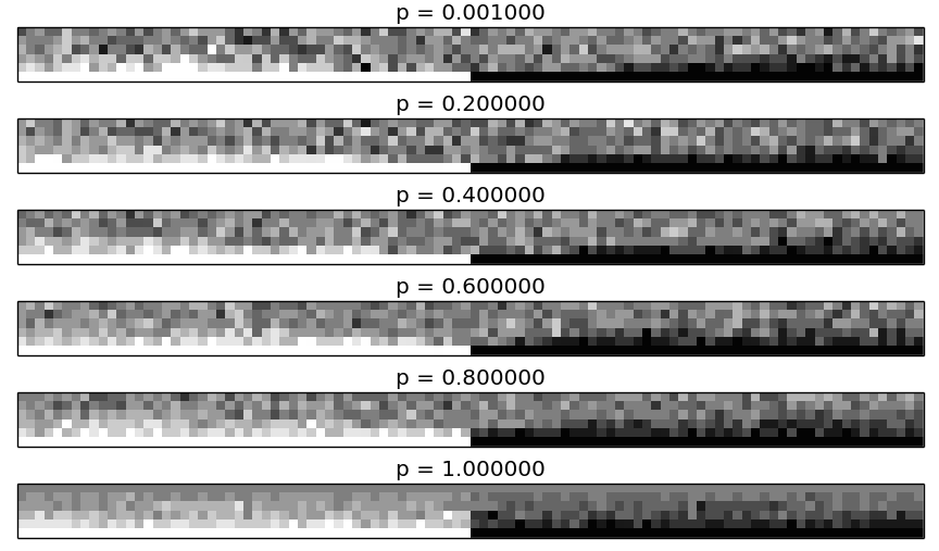
Figure 4: Point estimate of the density $\rho$ in a parallel TASEP after $T=2\frac{L}{p}\,\log L$ steps. The parameter $p$ ranges in $\{0.001,0.2,0.4,0.6,0.8,1.0\}$, while $\varepsilon$ ranges in $\{0,0.2,0.4,0.6,0.8,1\}$.

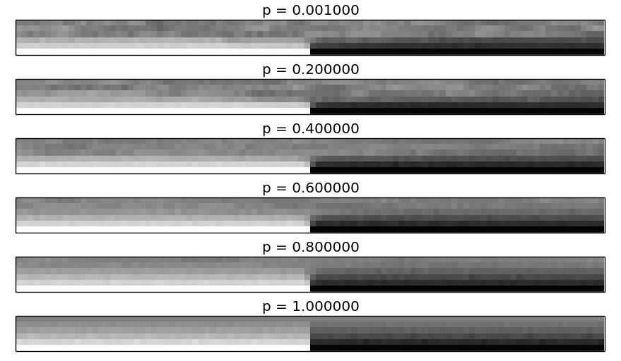
Figure 5: Mean density computed from 100 replicas of the dynamics The density is computed from the states visited by the dynamics between time $T$ and $T+100$, where $T=2\frac{L}{p}\,\log L$. The parameter $p$ ranges in $\{0.001,0.2,0.4,0.6,0.8,1.0\}$, while $\varepsilon$ ranges in $\{0,0.2,0.4,0.6,0.8,1\}$.

The diagrams in Figure 4 – one for each value of $p$ – are instantaneous plots of the configuration $\sigma$ at the time $T=2\frac{L}{p}\,\log L$. Each diagram is composed of 6 tiny rows showing the particle density for $\varepsilon\in\{0,0.2,0.4,0.6,0.8,1\}$. As expected, the last row of every diagram is split in half white-empty and half black-full dots due the total congestion of the blockage at $\varepsilon=1$.

Figure 5 is analogous to Figure 4 but it plots the average behaviour computed from $100$ density diagrams. Exactly like the previous graph, the first row corresponds to the complete absence of blockage, and its uniform colour fairly reflects the rotational invariance of the system.

These evidences seems to indicate the possibility that, although the current decreases for all $\epsilon$ (see [1]), the system seems to exhibit for $p<1$ a nearly-constant density up to a certain value of $\epsilon$, while after this value the density appears to be smaller in the first $L$ sites than in the second $L$. Such a difference in the density in the two halves of the ring is precisely what has emerged in Section 4 for the rule-184 cellular automaton ($p=1$) with an arbitrary blockage-intensity $\epsilon>0$, where the ph-symmetry plays a key role. Again, a complete understanding of this phenomenon should be based on the knowledge of the stationary measure in presence of a blockage.

The numerical evidences above show that there are many open interesting questions about our model, namely,

• prove that, in absence of blockage, the mixing time $\tau$ of the process is of the order of $\frac{L}{p}\,\log(L)$;

• show that except in the case $p=1$, i.e. $\omega\to\infty$, the probability to have a particle in a site is increasing along the circle starting from the blockage point;

• investigate, in the general case $p<1$, i.e. $\omega$ finite, the stationary measure of the system in presence of blockage. The last point may be possibly tackled via some perturbative approach with respect to the two cases that are completely known ($\varepsilon=0$ and $p=1$).

References

- [1] R. Basu, V. Sidoravicius, and A. Sly, Last passage percolation with a defect line and the solution of the slow bond problem, arXiv preprint arXiv:1408.3464, (2014).
- [2] O. Costin, J. Lebowitz, E. Speer, and A. Troiani, The blockage problem, arXiv preprint arXiv:1207.6555, (2012).
- [3] J. de Gier and B. Nienhuis, Exact stationary state for an asymmetric exclusion process with fully parallel dynamics, Physical Review E, 59 (1999), p. 4899.
- [4] B. Derrida, M. Evans, V. Hakim, and V. Pasquier, Exact solution of a 1D asymmetric exclusion model using a matrix formulation, Journal of Physics A: Mathematical and General, 26 (1993), p. 1493.
- [5] E. Duchi and G. Schaeffer, A combinatorial approach to jumping particles: The parallel tasep, Random Structures & Algorithms, 33 (2008), pp. 434–451.
- [6] M. Evans, Exact steady states of disordered hopping particle models with parallel and ordered sequential dynamics, Journal of Physics A: Mathematical and General, 30 (1997), p. 5669.
- [7] M. Evans, N. Rajewsky, and E. Speer, Exact solution of a cellular automaton for traffic, Journal of statistical physics, 95 (1999), pp. 45–96.
- [8] S. Janowsky and J. Lebowitz, Exact results for the asymmetric simple exclusion process with a blockage, Journal of Statistical Physics, 77 (1994), pp. 35–51.
- [9] S. A. Janowsky and J. L. Lebowitz, Finite-size effects and shock fluctuations in the asymmetric simple-exclusion process, Physical Review A, 45 (1992), p. 618.
- [10] C. Lancia and B. Scoppola, Equilibrium and non-equilibrium Ising models by means of PCA, Journal of Statistical Physics, 153 (2013), pp. 641–653.
- [11] T. M. Liggett, Interacting particle systems, Springer-Verlag, Berlin, 1985.
- [12] , Stochastic interacting systems: contact, voter and exclusion processes, vol. 324, Springer, 1999.
- [13] K. Mallick, Some exact results for the exclusion process, Journal of Statistical Mechanics: Theory and Experiment, 2011 (2011), p. P01024.
- [14] B. Morris, The mixing time for simple exclusion, The Annals of Applied Probability, (2006), pp. 615–635.
- [15] K. Nagel and M. Schreckenberg, A cellular automaton model for freeway traffic, Journal de physique I, 2 (1992), pp. 2221–2229.
- [16] A. Povolotsky and V. Priezzhev, Determinant solution for the totally asymmetric exclusion process with parallel update, Journal of Statistical Mechanics: Theory and Experiment, 2006 (2006), p. P07002.
- [17] , Determinant solution for the totally asymmetric exclusion process with parallel update: II. Ring geometry, Journal of Statistical Mechanics: Theory and Experiment, 2007 (2007), p. P08018.
- [18] A. Schadschneider, Traffic flow: a statistical physics point of view, Physica A: Statistical Mechanics and its Applications, 313 (2002), pp. 153–187.
- [19] M. Schreckenberg, A. Schadschneider, K. Nagel, and N. Ito, Discrete stochastic models for traffic flow, Physical Review E, 51 (1995), p. 2939.
- [20] G. Schütz and E. Domany, Phase transitions in an exactly soluble one-dimensional exclusion process, Journal of Statistical Physics, 72 (1993), pp. 277–296.
- [21] M. Woelki, The parallel TASEP, fixed particle number and weighted Motzkin paths, Journal of Physics A: Mathematical and Theoretical, 46 (2013), p. 505003.
- [22] M. Woelki and M. Schreckenberg, Exact matrix-product states for parallel dynamics: open boundaries and excess mass on the ring, Journal of Statistical Mechanics: Theory and Experiment, 2009 (2009), p. P05014.
- [23] S. Yukawa, M. Kikuchi, and S.-i. Tadaki, Dynamical phase transition in one dimensional traffic flow model with blockage, Journal of the Physical Society of Japan, 63 (1994), pp. 3609–3618.