The cosmic evolution of radio-AGN feedback to ${\mathbf{z}=1}$

Abstract

This paper presents the first measurement of the radio luminosity function of ‘jet-mode’ (radiatively-inefficient) radio-AGN out to $z=1$, in order to investigate the cosmic evolution of radio-AGN feedback. Eight radio source samples are combined to produce a catalogue of 211 radio-loud AGN with $0.5<z<1.0$, which are spectroscopically classified into jet-mode and radiative-mode (radiatively-efficient) AGN classes. Comparing with large samples of local radio-AGN from the Sloan Digital Sky Survey, the cosmic evolution of the radio luminosity function of each radio-AGN class is independently derived. Radiative-mode radio-AGN show an order of magnitude increase in space density out to $z\approx 1$ at all luminosities, consistent with these AGN being fuelled by cold gas. In contrast, the space density of jet-mode radio-AGN decreases with increasing redshift at low radio luminosities ($L_{\rm 1.4GHz}\mathrel{\hbox to0.0pt{\lower 3.0pt\hbox{$\mathchar 536\relax$}\hss}\raise 2.0pt\hbox{$\mathchar 316\relax$}}10^{24}$W Hz^-1) but increases at higher radio luminosities. Simple models are developed to explain the observed evolution. In the best-fitting models, the characteristic space density of jet-mode AGN declines with redshift in accordance with the declining space density of massive quiescent galaxies, which fuel them via cooling of gas in their hot haloes. A time delay of 1.5–2 Gyr may be present between the quenching of star formation and the onset of jet-mode radio-AGN activity. The behaviour at higher radio luminosities can be explained either by an increasing characteristic luminosity of jet-mode radio-AGN activity with redshift (roughly as $(1+z)^{3}$) or if the jet-mode radio-AGN population also includes some contribution of cold-gas-fuelled sources seen at a time when their accretion rate was low. Higher redshifts measurements would distinguish between these possibilities.

1 Introduction

Understanding the evolution of galaxies, from the end of the ‘dark ages’ through to the complexity and variety of systems we observe in the local Universe, remains a primary goal for observational and theoretical astrophysics. A crucial piece in the picture is the role that active galactic nuclei (AGN) play in controlling or terminating the star formation of their host galaxies (see reviews by Cattaneo et al., 2009; Fabian, 2012; Heckman & Best, 2014). Over recent years it has become clear that AGN activity falls into two fundamental modes, each of which may have a distinct ‘feedback’ role in galaxy evolution. Accretion at high fractions ($\mathrel{\hbox to0.0pt{\lower 3.0pt\hbox{$\mathchar 536\relax$}\hss}\raise 2.0pt\hbox{$\mathchar 318\relax$}}1$%) of the Eddington rate produces radiatively-efficient (quasar/Seyfert-like; hereafter ‘radiative-mode’) AGN, which display luminous radiation from a geometrically thin, optically thick accretion disk (e.g. Shakura & Sunyaev, 1973). Accretion at low Eddington fractions leads to an advection-dominated accretion flow (e.g. Narayan & Yi 1994, 1995); these AGN (hereafter ‘jet-mode’ AGN) are radiatively inefficient, and the bulk of their energetic output is in kinetic form, in two-sided collimated outflows (jets). For a full review of these two AGN populations, and their host galaxy properties, the reader is referred to Heckman & Best (2014).

The role of radiative-mode AGN in galaxy evolution remains hotly debated. These AGN are frequently invoked to quench star formation in massive galaxies, causing these to migrate from the locus of star-forming galaxies on to the red sequence (e.g. Silk & Rees, 1998; Hopkins et al., 2005; Springel et al., 2005; Schawinski et al., 2007; Cimatti et al., 2013). Models of this process can provide an explanation for the relationship seen between black hole mass and bulge velocity dispersion (Silk & Rees, 1998; Fabian, 1999; King, 2003). However, although there is ample evidence that radiative-mode AGN can drive winds (e.g. see reviews by Veilleux et al., 2005; Fabian, 2012), observational evidence for galaxy-scale feedback from radiative-mode AGN is so far limited to only the extreme, high luminosity systems, with little evidence that it occurs in more typical systems. Most radiative-mode AGN appear to be associated with star-forming galaxies, and to be fuelled by secular processes (Heckman & Best, 2014, and references therein). There are also indications that secular processes, rather than AGN activity, could be responsible for the quenching of star formation (‘mass-quenching’; Peng et al., 2010; Schawinski et al., 2014) and possibly setting up the black hole mass relations (e.g. Larson, 2010; Jahnke & Macciò, 2011). There remains much to be understood about whether radiative-mode AGN play any significant role in galaxy evolution.

In contrast, it is now widely accepted that recurrent jet-mode AGN activity is a fundamental component of the lifecycle of the most massive galaxies, responsible for maintaining these galaxies as ‘red and dead’ once they have migrated on to the red sequence (e.g. Croton et al., 2006; Bower et al., 2006; Best et al., 2006; Fabian et al., 2006). This is achieved by the radio jet depositing the AGN energy in kinetic form into the local intergalactic medium, through bubbles and cavities inflated in the surrounding hot gas (Böhringer et al., 1993; Carilli et al., 1994; McNamara et al., 2000; Fabian et al., 2003). This energy counteracts the radiative energy losses of that hot gas and prevents the bulk of the gas from cooling. This is most readily observed in the central galaxies of cool-core clusters (those with cooling times well below a Gyr, for which a counter-balancing heating source is required): in these systems, both radio AGN activity (Burns, 1990; Best et al., 2007) and X-ray cavities (Dunn & Fabian, 2006; Fabian, 2012) are almost universally present, and the current jet mechanical luminosity is seen to balance the cooling luminosity (see review by McNamara & Nulsen, 2007). The jet-mode AGN are believed to be fuelled primarily by the cooling of hot gas in the interstellar and intergalactic medium, and they deposit their energy back into this same hot gas, providing the necessary conditions for a feedback cycle (Heckman & Best, 2014, and references therein).

Amongst the general massive galaxy population, the prevalence of jet-mode AGN is a very strong function of both stellar mass ($M_{*}$) and black hole mass ($M_{\rm BH}$), with the fraction of galaxies hosting a jet-mode radio-AGN scaling as $M_{*}^{2.5}$ and as $M_{\rm BH}^{1.6}$ (Best et al., 2005; Janssen et al., 2012). In these systems, the instantaneous mechanical luminosity of the AGN jets can greatly exceed the cooling luminosity of the hot gas surrounding the galaxy, but if account is taken of the duty cycle of the recurrent activity then the time-averaged jet mechanical energy output is in closer agreement with the cooling losses (Best et al., 2006). The jet-mode AGN appear to act as a cosmic thermostat, being switched on whenever the cooling rate of the hot gas rises above some threshold, and acting to inhibit the gas cooling (and therefore switch off the AGN’s own gas supply as well). In the most massive galaxies, after the AGN switches off, the cooling quickly recommences, and so the AGN duty cycle is short and the prevalence of jet-mode AGN is high. In less massive galaxies, the AGN remains switched off for a longer time since the lower binding energy and gas sound speed lead to a longer recovery time before gas cooling and accretion recommence (e.g. Gaspari et al., 2013): these systems have a lower AGN prevalence, and oscillate around an equilibrium state.

This picture of jet-mode AGN activity has been established through detailed studies of the nearby Universe, and an important test of its validity is to examine whether it is consistent with observations at earlier cosmic times. An easily testable prediction of the model is that if jet-mode AGN are fuelled in the same manner at all redshifts, then the steep relationship between AGN prevalence and stellar mass ought to remain in place at higher redshift. Early studies of this, out to $z\mathrel{\hbox to0.0pt{\lower 3.0pt\hbox{$\mathchar 536\relax$}\hss}\raise 2.0pt\hbox{$\mathchar 316\relax$}}1$, indicate that the same relation is indeed seen (Tasse et al., 2008; Donoso et al., 2009; Simpson et al., 2013). A second measurable property is the cosmic evolution of the space density of jet-mode AGN. Phenomenological models of the dual-populations of AGN predict that the space density of jet-mode AGN activity should remain roughly flat out to moderate redshifts ($z\sim 1$; Croton et al., 2006; Merloni & Heinz, 2008; Körding et al., 2008; Mocz et al., 2013), but observationally this remains unconstrained. Measuring this is the focus of the current paper.

By far the best way to trace the cosmic evolution of the jet-mode AGN is through radio-selected samples, directly tracing the radio jet activity. The evolution of the radio luminosity function (RLF) of radio-loud AGN has been well-studied over many decades: it is known to be strongly luminosity dependent with the most powerful sources showing very rapid cosmic evolution (a factor $\sim$thousand increase in space density out to redshift 2–3; cf. Dunlop & Peacock, 1990; Rigby et al., 2011, and references therein), while less powerful sources show only a modest (factor 1.5–2) space density increase out to $z\sim 0.5$ (e.g. Sadler et al., 2007; Donoso et al., 2009) with a possible decline thereafter (Rigby et al., 2011; Simpson et al., 2012). However, the RLF is composed not only of jet-mode AGN, but also of the population of radio-loud radiative-mode AGN: these comprise the radio-loud quasars and their edge-on counterparts (often referred to as ‘High-Excitation Radio Galaxies’). In order to observationally determine the cosmic evolution of just the jet-mode AGN (‘Low-Excitation Radio Galaxies’), it is necessary to separate these two contributions to the overall RLF of radio-AGN.

Radiative-mode AGN dominate the radio-AGN population at higher radio luminosities where strong cosmic evolution is seen, while jet-mode radio-AGN dominate the radio population at lower radio luminosities, where cosmic evolution is far weaker. This has led many authors to consider a simple division in radio luminosity to separate the two radio populations. However, Best & Heckman (2012, hereafter BH12) used data from the Sloan Digital Sky Survey (SDSS; York et al., 2000; Strauss et al., 2002) to classify a local population of radio-AGN, and showed that both radiative-mode and jet-mode radio-AGN are found across all radio luminosities. They also provided evidence that, at a given radio luminosity, the two AGN classes show distinct cosmic evolution. This indicates that explicit separation of the two radio populations is needed to directly determine the cosmic evolution of jet-mode AGN alone.

This paper assembles and spectroscopically classifies a large sample of radio-AGN with $0.5<z<1.0$ across a broad range of radio luminosity, by combining eight radio surveys from the literature with high spectroscopic completeness, and adding additional spectroscopic observations. The samples are presented in Section 2, where the local comparison sample is also defined. Classification of the sources is described in Section 3. In Section 4, these data are used to determine the cosmic evolution of the RLF of jet-mode AGN, and simple models are developed to explain the observed evolution. The implications of the results are discussed in Section 5, and conclusions are drawn in Section 6. Throughout the paper, the cosmological parameters are assumed to have values of $\Omega_{m}=0.3$, $\Omega_{\Lambda}=0.7$, and $H_{0}=70$ km s^-1Mpc^-1.

2 Radio Source Samples

2.1 The local radio-AGN populations

BH12 combined spectroscopic data from the ‘main galaxy sample’ of the SDSS with radio data from the National Radio Astronomy Observatory (NRAO) Very Large Array (VLA) Sky Survey (NVSS; Condon et al., 1998) and the Faint Images of the Radio Sky at Twenty centimetres (FIRST) survey (Becker et al., 1995) to derive a sample of over 7000 radio-loud AGN in the local Universe. Both star-forming galaxies and radio-quiet quasars were excluded from their sample. Using the wide range of emission line flux measurements available for these sources, in conjunction with the line equivalent widths and the emission line to radio luminosity distributions, BH12 classified the sources as either jet-mode or radiative-mode radio-AGN.

BH12 determined the local RLFs for the two AGN classes. However, since their radio source sample was based upon the SDSS main galaxy sample it excluded both radio-loud quasars and broad-line radio galaxies; these can be dominant in the radiative-mode AGN population at higher radio luminosities. Gendre et al. (2013) also derived RLFs for jet-mode and radiative-mode sources, using the Combined NVSS-FIRST Galaxy catalogue (CoNFIG) which, although much smaller, did not suffer from this bias. They found broad agreement with BH12 except for the high luminosity radiative-mode AGN. For the analysis of this paper, therefore, the local RLFs were constructed using primarily the BH12 results, but replacing these for radiative-mode AGN above $L_{\rm 1.4GHz}=10^{26}$ W Hz^-1 by the steep-spectrum RLF determined from the Gendre et al. CoNFIG data (cf. Heckman & Best, 2014). The resultant (steep-spectrum) local RLFs are shown in Figure 1, along with the best-fitting broken power law models of the form

$$\rho=\frac{\rho_{0}}{(L/L_{0})^{\beta}+(L/L_{0})^{\gamma}}$$

where $L_{0}$ is a characteristic luminosity and $\rho$ and $\rho_{0}$ are measured in units of number of sources per log${}_{10}L$ per Mpc³.

The BH12 sample also provides the basis for the optimisation of emission line ratio diagnostics in Section 3 to segregate the jet-mode and radiative-mode sources at the higher redshifts (where far fewer emission line fluxes are available).

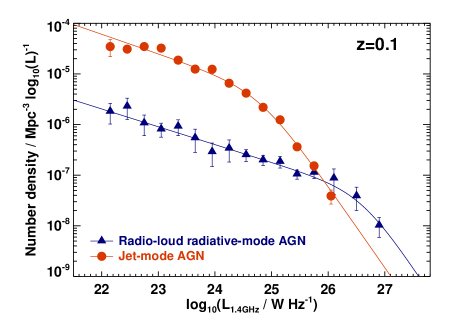
Figure 1: The local radio luminosity functions for the radiative-mode and jet-mode radio-AGN separately, along with best-fitting broken power-law models (adapted from Heckman & Best, 2014).

2.2 A combined radio source sample at ${\mathbf{0}.5<z<1.0}$

Eight separate radio surveys with a wide range of flux density limits were combined in order to develop a large total radio source sample covering a broad span of radio luminosities. Each of these surveys was selected to have high spectroscopic completeness from which galaxies in the target redshift range $0.5<z<1.0$ could be drawn. Where necessary, each sample was re-selected at 1.4 GHz, as described below, to produce a sample which would be complete for steep-spectrum sources down to a fixed 1.4 GHz flux density limit over the same sky area as the original sample. This re-selection avoids selection biases in the analysis.

Despite the use of the highest spectroscopic completeness samples available, a significant number of radio sources lacked either spectroscopic redshifts or available spectra of sufficient quality to allow classification as jet-mode or radiative-mode. A programme of spectroscopic follow-up observations was therefore carried out, targeting objects which either lacked classification, or which had photometric redshifts within (or very close to) the target range $0.5<z<1.0$. This spectroscopic programme was carried out on the William Herschel Telescope (WHT) during two runs in 2012; details of the observations and the results arising are described in Appendix B. On the basis of these new observations, some sources were removed from the samples as their spectroscopic redshifts placed them outside the required range. Details of these excluded sources are given in Table 8. In the descriptions of the 8 samples that follows, these objects are already excluded when discussing numbers of sources.

Table 1: Properties of the radio surveys used for the construction of the $0.5<z<1.0$ sample.

Survey	Sky area	Flux density lim.	No of sources
	(sr)	(mJy, 1.4 GHz)	($0.5<z<1.0$)
WP85r	9.81	4000	29
CoNFIG-1	1.50	1300	45
CoNFIG-2r	0.89	800	24
PSRr	0.075	500	9
7CRSr	0.022	167	21
TOOT-00r	0.0015	33	7
CENSORS	0.0018	7.2	28
Hercules	0.00038	2.0	16
SXDS	0.000247	0.2	32

2.2.1 Wall & Peacock sample

The original Wall & Peacock (1985) radio source sample contained 233 radio sources brighter than 2.0 Jy at 2.7 GHz over 9.81 sr of sky. From this, Rigby et al. (2011) re-selected a sample of 138 steep spectrum ($\alpha>0.5$) radio sources which was complete to a flux density limit of 4 Jy at 1.4 GHz. This re-selected sample, hereafter referred to as WP85r, is 97% spectroscopically complete, and contains 29 sources in the redshift range $0.5<z<1.0$ (including one photometric redshift source).

2.2.2 CoNFiG sample

The CoNFIG catalogue was presented by Gendre et al. (2010) and consists of four different radio source samples selected at 1.4 GHz from the NVSS at different flux density levels. Here, the CoNFiG-1 sample is used, along with the revised ‘CoNFIG-2r’ sample defined by Ker et al. (2012). CoNFiG-1 is complete to a 1.4 GHz flux density limit of 1.3 Jy. CoNFiG-2r corresponds to the subset of CoNFiG-2 with flux densities in the range 0.8 Jy $<S_{\rm 1.4GHz}<$ 1.3 Jy; the lower flux density limit is set because at fainter flux densities CoNFIG-2 becomes rapidly more incomplete in terms of optical identifications and redshift estimates, while sources brighter than 1.3 Jy are already in CoNFIG-1 since the sky areas overlap. The combined CoNFIG-1 and CoNFIG-2r samples contain 6 steep spectrum sources without optical identification, but the magnitude limits indicate that these have redshifts $z\mathrel{\hbox to0.0pt{\lower 3.0pt\hbox{$\mathchar 536\relax$}\hss}\raise 2.0pt\hbox{$\mathchar 318\relax$}}1$ (see discussion in Ker et al., 2012), so these sources are discounted for the current analysis. Excluding also three further sources which are duplicates of WP85r sources (3C196, 3C237, 3C280), there are 45 CoNFIG-1 and 24 CoNFIG-2r sources with spectroscopic (60) or photometric (9) redshifts in the range $0.5<z<1.0$.

2.2.3 Parkes Selected Regions sample

The original Parkes Selected Regions sample (Wall et al., 1971; Downes et al., 1986; Dunlop et al., 1989) was defined at 2.7 GHz and contains 178 radio sources brighter than 0.1 Jy over 0.075 sr of sky. Rigby et al. (2011) re-selected the sample at 1.4 GHz to produce a complete sample of 59 steep spectrum ($\alpha>0.5$) sources above a flux density of $S_{\rm 1.4GHz}=0.36$ Jy. 20 of these sources have redshifts in the redshift range $0.5<z<1.0$. However, at the faintest flux densities the spectroscopic classification fraction is low, so the sample used here (referred to as PSRr) is restricted to the 9 sources above $S_{\rm 1.4GHz}=0.50$ Jy.

2.2.4 7C Redshift Survey sample

The Seventh Cambridge Redshift Survey, 7CRS, is composed of three subsamples, 7CI, 7CII and 7CIII, over three different sky areas totalling 0.022 sr, each selected at 151 MHz down to a limiting flux density limit of around 0.5 Jy (Willott et al., 2002; Lacy et al., 1999, and references therein). This sample was re-selected at 1.4 GHz down to a flux density of $S_{\rm 1.4GHz}=0.167$ Jy. Although this re-selection removes a large fraction of the 7CRS sample, the remaining sample will be complete for steep spectrum ($\alpha>0.5$) sources, and populates an otherwise sparsely-sampled range of radio luminosities. 21 sources from the re-selected sample, hereafter referred to as 7CRSr, have redshifts (all spectroscopic) in the target range.

2.2.5 Tex-Ox One Thousand sample

The Tex-Ox One Thousand (TOOT) survey (Hill & Rawlings, 2003) was an ambitious attempt to measure spectroscopic redshifts for 1000 galaxies down to $S_{\rm 151MHz}=0.1$ Jy; so far only results in the TOOT-00 field have been published (Vardoulaki et al., 2010). The sample, over a sky area of 0.0015 sr, has been re-selected at 1.4 GHz down to a flux density limit of 0.033 Jy, above which it will be complete for steep spectrum sources. 7 sources in this re-selected (TOOT-00r) sample lie between redshifts 0.5 and 1.0 (all spectroscopically confirmed).

2.2.6 CENSORS sample

The Combined EIS-NVSS Survey of Radio Sources (CENSORS) is a 1.4 GHz-selected sample of 135 radio sources down to a flux density limit of 0.0072 Jy, over the 0.0018 sr sky region that overlaps the ESO Imaging Survey (EIS) patch D (Best et al., 2003; Brookes et al., 2006, 2008; Rigby et al., 2011). At nearly 80% spectroscopically complete, it is one of the most complete faint radio source samples available. 28 of these sources lie in the redshift range $0.5<z<1.0$ (including four photometric redshifts).

2.2.7 Hercules sample

The Hercules sample is taken from a field in the Leiden-Berkeley Deep Survey (Windhorst et al., 1984), and consists of 64 sources selected to have a flux density greater than 0.002 Jy at 1.4 GHz (Waddington et al., 2001). The surveyed sky area is 0.00038 sr. 16 of these sources have spectroscopic (14) or photometric (2) redshifts between 0.5 and 1.0.

2.2.8 SXDF sample

A deep 1.4 GHz radio survey of the Subaru/XMM-Newton Deep Field, which overlaps the United Kingdom Infrared Deep Sky Survey (UKIDSS; Lawrence et al., 2007) Ultra-Deep Survey (UDS) region, has been carried out by Simpson et al. (2006). These data reach a depth of 12$\mu$Jy rms in the central regions, with the catalogue complete to the 100$\mu$Jy level (for point sources) over the whole field. Spectroscopic and photometric redshift data for the detected radio sources were presented by Simpson et al. (2012). The spectroscopic completeness decreases at lower flux densities, so to reduce the number of unclassified sources, the current analysis was restricted to sources with an integrated flux density level above $S_{\rm 1.4GHz}=0.0002$ Jy, over the survey area of 0.000247 sr. This flux density cut also reduces the risk of missing faint extended sources. Within the redshift range $0.5<z<1.0$, 38 sources were selected.

At the depth of this survey, starbursting galaxies and radio-quiet quasars (both optically obscured and unobscured) are expected to contribute a significant fraction of the radio source population (their contribution to other brighter samples is expected to be negligible). Simpson et al. (2012) identified starburst galaxies within the sample from their emission line ratios and absorption line properties. Radio-quiet quasars can be identified on the basis of the ratio between their mid-infrared 24$\mu$m flux density and their radio flux density (the $q_{24}$ parameter, where $q_{24}={\rm log}_{10}(S_{24\mu m}/S_{\rm 1.4GHz})$ and $S_{24\mu m}$ and $S_{\rm 1.4GHz}$ are each k-corrected values). Star-forming galaxies and radio-quiet quasars both display a narrow distribution in this parameter (e.g. Appleton et al., 2004; Ibar et al., 2008; Simpson et al., 2012), while radio-loud AGN are offset to lower values. $q_{24}$ values for the SXDF were calculated by Simpson et al. (2012) and the threshold value of $q_{24}=-0.23$ determined by Ibar et al. (2008) was adopted to remove objects with higher $q_{24}$ values. In this manner, a clean sample of 27 radio-loud AGN was selected in the target redshift range (including 5 sources with photometric redshifts).

2.2.9 Summary of combined sample

The combined $0.5<z<1.0$ sample contains 211 radio sources (including 27 with photometric redshifts). The properties of these sources are provided in Table 6 and their distribution on the radio luminosity versus redshift plane is shown in Figure 2.

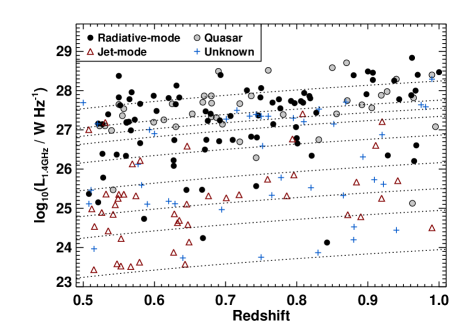
Figure 2: The distribution of the combined radio sample on the radio luminosity versus redshift plane. Sources are classified as radiative-mode and jet-mode where possible. Sources classified as quasars are plotted with separate symbols but form part of the radiative-mode class. The dotted lines indicate the luminosity limits of the different samples as a function of redshift for a spectral index $\alpha=0.75$.

3 Classification of the radio sources

The classification of radio galaxies as radiative-mode or jet-mode can be carried out using emission line strengths and line flux ratios. In the nearby Universe, the high quality of the SDSS spectroscopic data allowed BH12 to derive reliable classifications using the emission line ratio diagnostic diagrams that are generally adopted to separate Low-Ionisation Nuclear Emission-line Regions (LINERs; Heckman, 1980) from Seyfert galaxies (Kewley et al., 2006; Buttiglione et al., 2010; Cid Fernandes et al., 2010; Baldi & Capetti, 2010). However, for the higher redshift samples, the observed wavelength range and the lower quality of the spectra generally prohibit detection or measurement of some emission lines required. Separation of the two populations has typically been performed using either a single emission line flux ratio ($f_{\rm[OIII]5007}/f_{H\alpha}$ or $f_{\rm[OIII]5007}/f_{\rm[OII]3727}$) or a single line equivalent width (EW_[OIII]), with different authors adopting slightly different criteria (e.g. Laing et al., 1994; Jackson & Rawlings, 1997; Tadhunter et al., 1998).

For the $0.5<z<1.0$ sample, the [OII] 3727 line is available in all optical spectra, and the [OIII] 5007 line in most. These lines therefore form the basis of the classifications used in this paper. The BH12 data can be used to optimally calibrate the separation criteria using the line flux ratio of these two lines, and their rest-frame equivalent widths. For these analyses, the subsample of BH12 sources used was those with [OII] 3727 and [OIII] 5007 emission lines detected with S/N $>$ 5 and which were classified solely on the basis of emission line ratio diagnostics. The left panel of Figure 3 shows a plot of EW_[OIII] vs $f_{\rm[OIII]5007}/f_{\rm[OII]3727}$ for this BH12 subsample, and demonstrates that where both emission lines are available, the cleanest separation adopts a combination of these parameters, rather than either individually. The division line adopted here is

$${\rm log}_{10}\left({\rm EW}_{\rm[OIII]}\right)=0.7-3.3{\rm log}_{10}\left(\frac{f_{\rm[OII]5007}}{f_{\rm[OIII]3727}}\right).$$

The parameters of this division line were derived by minimising the quantity $f_{\rm wrong}=\left(f_{\rm jet-wrong}^{2}+f_{\rm rad-wrong}^{2}\right)^{1/2}$ where $f_{\rm jet-wrong}$ and $f_{\rm rad-wrong}$ are the fraction of wrongly-classified jet-mode and radiative-mode AGN respectively.

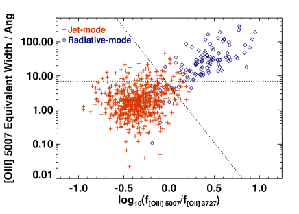
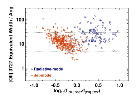
Figure 3: The distribution of low-redshift radiative-mode and jet-mode AGN from BH12 on emission-line ratio versus equivalent width plots, for the [OIII] 5007 and [OII] 3727 emission lines. These are used to calibrate the classification division lines adopted for the high redshift samples (see Section 3).

This classification criterion is adopted for spectra where flux measurements of both lines are available. If only the [OIII] line is available, or the spectra are not flux calibrated, then the classification was made solely on EW_[OIII], with a division at 7Å (again, this value was derived by minimising $f_{\rm wrong}$). Finally, if only the [OII] line is available, then the division was made using EW_[OII]. As shown in the right panel of Figure 3, the two populations overlap significantly in that parameter. Therefore objects with EW${}_{\rm[OII]}>30$Å were classified as radiative-mode AGN, those with EW${}_{\rm[OII]}<5$Å were classified as jet-mode AGN, but those with equivalent widths between these two limits were considered unclassifiable.

An extensive literature search was carried out to locate spectra for sources within the samples used. For sources with available spectra in electronic form, or with tabulated line properties, the above criteria were applied. For some sources the only available spectra were in paper form: most of these were powerful radio sources with very strong lines whose classification as radiative-mode was unambiguous, in which case they were classified by eye. The remainder were left unclassified. Some sources which lacked either a spectrum or a classification were targeted in the new WHT spectroscopic observations (see Appendix B) and were classified on that basis. Note that for some sources spectra exist but without a redshift having been determined. If these were of sufficient quality to rule out the presence of an emission line with EW $>5$Å then the source was classified as a jet-mode AGN, otherwise it was left unclassified. The final classifications for each source are listed in Table 6. In total it was possible to classify 123 sources as radiative-mode and 46 sources as jet-mode, with 42 sources remaining unclassifiable.

4 The evolving radio luminosity functions of radio-AGN populations

4.1 Deriving the radio luminosity functions

Radio luminosity functions were calculated using the standard technique, $\rho=\sum_{i}1/V_{i}$ (Schmidt, 1968; Condon, 1989), where $V_{i}$ is the volume within which source $i$ could be detected. For the higher redshift samples, the calculation of $V_{i}$ requires careful accounting of the combination of different survey areas and depths, since sources detected in one survey may have been detectable (and therefore have a contribution to $V_{i}$) in another survey. For a given survey, a source of given luminosity and spectral index is detectable out to the redshift ($z_{\rm lim}$) at which its radio flux density drops below the flux limit of that survey. If the RLF is being calculated within a redshift range $z_{\rm min}<z<z_{\rm max}$ (typically $0.5<z<1.0$ in this paper), then: (i) if $z_{\rm lim}<z_{\rm min}$ the source could not be detected by this survey in the redshift range studied; (ii) if $z_{\rm lim}>z_{\rm max}$ then the source could be detected over the entire volume probed by that survey between $z_{\rm min}$ and $z_{\rm max}$; (iii) if $z_{\rm min}\leq z_{\rm lim}\leq z_{\rm max}$ then the source could be detected over the subset of the volume between $z_{\rm min}$ and $z_{\rm lim}$. The total $V_{i}$ for each source is calculated by summing the contributions to the detectable volume from all of the eight surveys, taking account of any overlapping sky areas.

The RLFs were also parameterised with broken power-law fits ($\rho=\rho_{0}/[(L/L_{0})^{\beta}+(L/L_{0})^{\gamma}]$). These parameterised fits were determined using a maximum-likelihood analysis (cf. Marshall et al., 1983), specifically by minimising the function

$$S=-2\sum_{i=1}^{N}\ln\rho(L_{i},z_{i},\alpha_{i})$$

$$\qquad\qquad+2\int\!\!\!\int\!\!\!\int\rho(L,z,\alpha)\frac{{\rm d}V(L,z,\alpha)}{{\rm d}z}{\rm d}z\,{\rm d}(\log_{10}L)\,{\rm d}\alpha$$

where $\rho(L,z,\alpha)$ is the space density of sources of luminosity $L$ and spectral index $\alpha$ at redshift $z$, and $\frac{{\rm d}V(L,z,\alpha)}{{\rm d}z}$ is the co-moving volume available between redshift $z$ and $z+{\rm d}z$ for sources of luminosity $L$ and spectral index $\alpha$, taking into account the sky areas and flux density limits of the different constituent surveys. The first term is therefore the sum of $\ln\rho$ over the $N$ sources in the sample, while the second term integrates the model distribution and should evaluate to approximately $2N$ for good fits.

The distribution in spectral index was assumed to be independent of both radio luminosity and redshift (over the narrow redshift range sampled), and was evaluated as a Gaussian centred on $\alpha=0.75$, with standard deviation 0.15, cutting to zero below $\alpha=0.5$ due to the steep-spectrum selection limit. Tests indicate that the results are unaffected if other sensible choices are adopted instead. For fitting of the RLF broken power-law parameters at different redshifts, $\rho$ was assumed to be independent of redshift within each studied redshift bin. For some fits the value of $\gamma$ was fixed at 1.7 (consistent with the best-fit values, and a reasonable fit in all cases) to ease the degeneracies between the different parameters.

Marginalised errors on the parameter values were derived from the covariance matrix, $\sigma^{2}_{\rm marg,i}=([H]^{-1})_{ii}$ where $H_{ij}=\frac{-\partial^{2}S}{\partial p_{i}\partial p_{j}}$ is the Hessian matrix (for parameters $p_{i}$) which was evaluated numerically. As well as these marginalised errors, however, a significant source of uncertainty arises from the presence of unclassified sources. To account for these, the maximum likelihood analysis was carried out 1000 times, each time randomly including or excluding each unclassified source (with equal probability). The best-fit value for each parameter was determined by taking the mean of these 1000 analyses. The uncertainty on the parameter value was derived by combining the mean value of the marginalised error for that parameter in quadrature with the standard deviation of the parameter values determined from the 1000 iterations of the analysis. In general the marginalised error was the dominant source of error, indicating that small sample size and parameter degeneracies were more important sources of error than the missing classifications.

4.2 Radio luminosity functions results

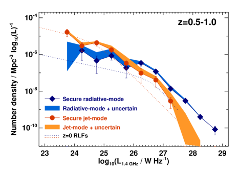
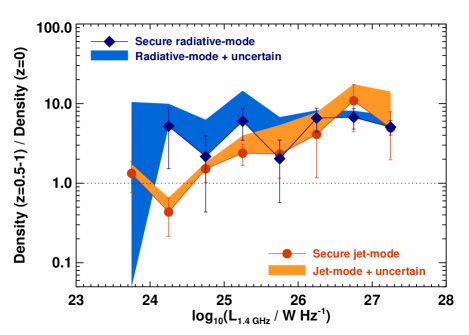
Figure 4: Top: the RLFs of jet-mode and radiative-mode radio-AGN at $0.5<z<1.0$, compared with the local RLFs of the same populations. Bottom: the ratio of the space density of jet-mode and radiative-mode AGN at $0.5<z<1.0$, compared to the local Universe, as a function of radio luminosity. In both panels the data points and associated error bars represent the measured space density and its Poisson uncertainty, based solely on the securely-classified objects, while the shaded region represents the potential increase in space density arising from inclusion of all unclassified objects.

Table 2: The $0.5<z<1.0$ radio luminosity functions at 1.4 GHz, derived separately for the jet-mode and radiative-mode populations. Column 1 indicates the range of 1.4 GHz radio luminosities of each bin. Column 2 gives the total number of radio sources in that radio luminosity range and Column 3 gives the associated space density, in units of number per log${}_{10}L$ per Mpc³. Columns 4 to 9 show the equivalent values for radiative-mode radio-AGN, jet-mode radio-AGN and unclassified radio-AGN, respectively. Uncertainties are statistical Poissonian uncertainties only (see also Figure 4). Note that one jet-mode source has $L_{\rm 1.4GHz}<10^{23.5}$W Hz^-1, so the number of sources in the table sums to only 210.

${\rm log}L_{\rm 1.4GHz}$	All radio sources		Radiative-mode		Jet-mode		Unclassified
W Hz-1	N	${\rm log}_{10}\rho$	N	${\rm log}_{10}\rho$	N	${\rm log}_{10}\rho$	N	${\rm log}_{10}\rho$
23.5-24.0	10	-$4.67^{+0.13}_{-0.19}$	0		6	-$4.79^{+0.16}_{-0.24}$	4	-$5.30$
24.0-24.5	8	-$5.21^{+0.13}_{-0.19}$	2	-$5.78^{+0.23}_{-0.53}$	4	-$5.53^{+0.18}_{-0.30}$	2	-$5.82$
24.5-25.0	13	-$5.25^{+0.11}_{-0.15}$	1	-$6.34^{+0.26}_{-0.70}$	10	-$5.36^{+0.12}_{-0.17}$	2	-$6.06$
25.0-25.5	25	-$5.41^{+0.08}_{-0.10}$	6	-$6.07^{+0.15}_{-0.24}$	12	-$5.74^{+0.11}_{-0.15}$	7	-$5.92$
25.5-26.0	11	-$6.02^{+0.12}_{-0.16}$	2	-$6.73^{+0.24}_{-0.55}$	4	-$6.48^{+0.18}_{-0.30}$	5	-$6.36$
26.0-26.5	14	-$6.28^{+0.11}_{-0.14}$	10	-$6.46^{+0.12}_{-0.18}$	2	-$7.01^{+0.23}_{-0.55}$	2	-$7.06$
26.5-27.0	20	-$6.73^{+0.09}_{-0.12}$	14	-$6.93^{+0.11}_{-0.15}$	3	-$7.39^{+0.20}_{-0.39}$	3	-$7.60$
27.0-27.5	45	-$7.65^{+0.07}_{-0.08}$	30	-$7.86^{+0.08}_{-0.10}$	4	-$8.54^{+0.20}_{-0.40}$	11	-$8.27$
27.5-28.0	43	-$8.44^{+0.07}_{-0.08}$	38	-$8.52^{+0.07}_{-0.08}$	0		5	-$9.20$
28.0-28.5	17	-$9.37^{+0.10}_{-0.13}$	16	-$9.40^{+0.10}_{-0.13}$	0		1	-$10.68$
28.5-29.0	4	-$10.08^{+0.18}_{-0.30}$	4	-$10.08^{+0.18}_{-0.30}$	0		0

Table 3: Parameters of broken power law fits to the 1.4 GHz radio luminosity functions, of the form $\rho=\rho_{0}/[(L/L_{0})^{\beta}+(L/L_{0})^{\gamma}]$, where $\rho$ and $\rho_{0}$ are measured in units of number per log${}_{10}L$ per Mpc³. For some fits, the value of $\gamma$ is fixed at 1.7.

AGN-type	Redshift	$L_{0}$	log${}_{10}(\rho_{0})$	$\beta$	$\gamma$
All	$z<0.3$	$24.95\pm 0.14$	-$5.33\pm 0.12$	$0.42\pm 0.04$	$1.66\pm 0.21$
	$0.5<z<1.0$	$26.22\pm 0.14$	-$5.96\pm 0.16$	$0.45\pm 0.06$	$1.68\pm 0.06$
Jet-mode	$z<0.3$	$24.81\pm 0.18$	-$5.30\pm 0.17$	$0.39\pm 0.06$	$1.61\pm 0.19$
	$0.5<z<1.0$	$25.50\pm 0.14$	-$5.62\pm 0.16$	$0.35\pm 0.12$	1.70 (fixed)
	$0.5<z<0.7$	$25.11\pm 0.15$	-$5.15\pm 0.19$	$0.28\pm 0.14$	1.70 (fixed)
	$0.7<z<1.0$	$25.77\pm 0.19$	-$5.86\pm 0.26$	$0.13\pm 0.24$	1.70 (fixed)
Radiative-mode	$z<0.3$	$26.62\pm 0.11$	-$7.32\pm 0.08$	$0.35\pm 0.02$	1.70 (fixed)
	$0.5<z<1.0$	$26.45\pm 0.11$	-$6.37\pm 0.17$	$0.30\pm 0.10$	1.70 (fixed)

The derived $0.5<z<1.0$ RLFs of the radiative-mode, jet-mode and unclassified radio-AGN are tabulated separately in Table 2. The RLFs are also shown in the upper panel of Figure 4: the data points indicate the RLFs of the securely classified objects, with associated error bars, while the shaded regions indicate the extent to which these might be increased by inclusion of the unclassified objects. The parameters of the broken power-law fits (calculated using the method of Section 4.1) are given in Table 3. The fits to the local RLFs are also shown in Figure 4, from which the cosmic evolution of the RLFs of each class can be seen. This is more clearly demonstrated in the lower panel of Figure 4 which shows the ratio of the high-to-low redshift RLFs in terms of a space-density scaling factor as a function of radio luminosity.

The radiative-mode radio-AGN evolve by a constant factor of $\approx 7$ in co-moving space density, between the local Universe and $z\approx 0.75$, at all radio luminosities. At high radio luminosities (where these sources dominate) this is entirely consistent with previous determinations of the evolution of the total RLF (Dunlop & Peacock, 1990; Rigby et al., 2011). The RLF fits data prefer a pure density evolution model, with little change in $L_{0}$, although sufficient parameter degeneracy remains for the radiative-mode AGN fitting that a combination of density and luminosity evolution cannot be ruled out.

The evolution of the jet-mode radio-AGN is rather more complicated. At low radio luminosities ($L_{\rm 1.4GHz}\mathrel{\hbox to0.0pt{\lower 3.0pt\hbox{$\mathchar 536\relax$}\hss}\raise 2.0pt\hbox{$\mathchar 316\relax$}}10^{25}$W Hz^-1), these show little or no cosmic evolution. This is in line with the previous measurements of the low evolution of the RLF as a whole at these low luminosities (Sadler et al., 2007; Donoso et al., 2009), since the jet-mode AGN dominate the overall population. Indeed, the mild evolution seen here in the total RLF is mostly driven by the strong evolution of the sub-dominant radiative-mode population. At higher radio luminosity, however, the jet-mode AGN do show significant cosmic evolution, approaching that of the radiative-mode AGN.

Figure 5 considers the RLF of the jet-mode AGN, now split into two redshift ranges: $0.5<z<0.7$ and $0.7<z<1.0$ (see also Table 4). It is evident that at the lowest radio luminosities ($L_{\rm 1.4GHz}\mathrel{\hbox to0.0pt{\lower 3.0pt\hbox{$\mathchar 536\relax$}\hss}\raise 2.0pt\hbox{$\mathchar 316\relax$}}10^{24}$W Hz^-1) the space density of jet-mode AGN remains broadly constant out to $z\approx 0.5$ and then decreases to $z=1$. At moderate luminosities ($10^{24}$W Hz${}^{-1}\mathrel{\hbox to0.0pt{\lower 3.0pt\hbox{$\mathchar 536\relax$}\hss}\raise 2.0pt\hbox{$\mathchar 316\relax$}}L_{\rm 1.4GHz}\mathrel{\hbox to0.0pt{\lower 3.0pt\hbox{$\mathchar 536\relax$}\hss}\raise 2.0pt\hbox{$\mathchar 316\relax$}}10^{26}$W Hz^-1) the space density increases to $z\sim 0.5$ before falling. At the highest luminosities, the space density continues to increase with increasing redshift out to $z\sim 1$. This is consistent with the luminosity-dependent evolution of the overall RLF seen by Rigby et al. (2011) but does indicate that the picture is more complicated than just differential evolution of two different AGN populations.

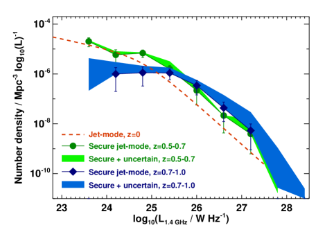
Figure 5: Top: the RLF of jet-mode radio-AGN at $0.5<z<0.7$ and $0.7<z<1.0$ compared with that in the local Universe. Errors bars and shaded regions are as defined in Fig 4.

Table 4: The 1.4 GHz radio luminosity functions of jet-mode AGN split into $0.5<z<0.7$ and $0.7<z<1.0$ redshift bins. Column 1 indicates the range of 1.4 GHz radio luminosities of each bin. Columns 2-5 show the results for the $0.5<z<0.7$ bin, with the columns indicating respectively the number of jet-mode AGN, their space density (in units of number per log${}_{10}L$ per Mpc³), the number of unclassified sources, and their space density. Columns 6-9 repeat these results for the higher redshift range.

${\rm log}L_{\rm 1.4GHz}$	…………..$0.5<z<0.7$…………..				…………..$0.7<z<1.0$…………..
W Hz-1	Jet-mode		Unclassified		Jet-mode		Unclassified
	N	${\rm log}_{10}\rho$	N	${\rm log}_{10}\rho$	N	${\rm log}_{10}\rho$	N	${\rm log}_{10}\rho$
23.3-23.9	7	-$4.69^{+0.14}_{-0.22}$	1	-$5.65$	0		2	-$5.37$
23.9-24.5	3	-$5.23^{+0.20}_{-0.39}$	1	-$5.65$	1	-$6.00^{+0.26}_{-0.70}$	2	-$5.70$
24.5-25.1	10	-$5.16^{+0.13}_{-0.18}$	1	-$6.33$	2	-$5.95^{+0.23}_{-0.54}$	1	-$6.00$
25.1-25.7	6	-$5.81^{+0.15}_{-0.23}$	6	-$5.78$	5	-$5.96^{+0.17}_{-0.27}$	4	-$6.16$
25.7-26.3	2	-$6.66^{+0.24}_{-0.58}$	1	-$6.85$	3	-$6.47^{+0.20}_{-0.37}$	2	-$6.64$
26.3-26.9	1	-$7.67^{+0.26}_{-0.70}$	0		2	-$7.36^{+0.23}_{-0.55}$	3	-$7.00$
26.9-27.5	2	-$8.41^{+0.26}_{-0.80}$	3	-$7.93$	2	-$8.27^{+0.26}_{-0.78}$	9	-$7.62$

4.3 Modelling the jet-mode RLF evolution

4.3.1 A pure density evolution model

In the simplest picture of the jet-mode radio-AGN population, these AGN are hosted by quiescent galaxies living within hot gas haloes, in which star-formation has been largely extinguished, and the AGN is fuelled by the cooling of the hot gas (see Section 1). In this picture, it is possible to predict the evolution in the space density of jet-mode AGN from the evolution of potential host galaxies. In recent years there have been a number of observational determinations of the stellar mass function of quiescent galaxies both in the local Universe (e.g. Baldry et al., 2012) and out to high redshifts (e.g. Domínguez Sánchez et al., 2011; Moustakas et al., 2013; Ilbert et al., 2013; Muzzin et al., 2013). These stellar mass functions can be combined with the prevalence of jet-mode AGN activity as a function of stellar mass ($f_{\rm AGN}\approx 0.01(M_{*}/10^{11}M_{\odot})^{2.5}$; Best et al., 2005; Janssen et al., 2012) to predict the evolution of the space density of jet-mode AGN as a function of redshift.

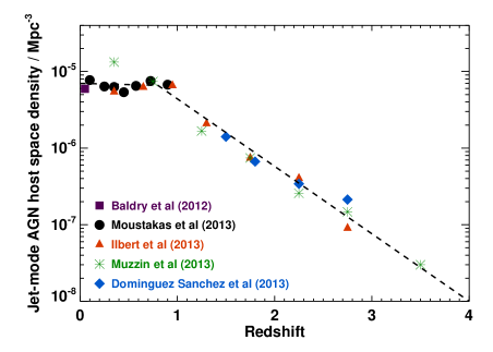
Figure 6: Cosmic evolution of the space density of potential hosts of jet-mode AGN, derived by combining the stellar mass functions of quiescent galaxies at different redshifts (from Domínguez Sánchez et al., 2011; Baldry et al., 2012; Moustakas et al., 2013; Ilbert et al., 2013; Muzzin et al., 2013) with the prevalence of jet-mode AGN activity as a function of stellar mass ($f_{\rm AGN}\approx 0.01(M/10^{11}M_{\odot})^{2.5}$; Best et al., 2005; Janssen et al., 2012). All quiescent galaxy stellar mass functions are first converted onto a Chabrier IMF. The results from Moustakas et al. (2013) are scaled down by a factor of two, and those of Domínguez Sánchez et al. (2011) by a factor of 1.5 to bring the different datasets into agreement for visualisation – but the form of the fitted redshift evolution (dashed line) is consistent across all datasets.

Figure 6 shows the result of this analysis. To derive this, the literature mass functions were shifted in mass (where necessary) to move then all onto a Chabrier IMF. Furthermore, to bring different datasets in to line with each other for visualisation purposes (differences are likely to be due to different definitions of quiescent galaxies), it was necessary to vertically shift the data points of Moustakas et al. (2013) down by a factor of two, and those of Domínguez Sánchez et al. (2011) down by a factor of 1.5. These corrections means that the absolute values of the plotted space densities may be unreliable, but the trends with redshift are robust, as these are consistent across all datasets. The space density of jet-mode AGN hosts is modelled in a simple manner as evolving as $(1+z)^{-0.1}$ out to redshift $z=0.8$, and then as $(1+z)^{-6.5}$ at higher redshifts. A similar result is obtained if one instead simply considers the evolution of the space density of all quiescent galaxies more massive than $10^{10}M_{\odot}$.

Under this simplest picture of jet-mode AGN evolution, the jet-mode RLF will demonstrate pure density evolution, evolving down in space density in accordance with the cosmic evolution of the potential host galaxies, just derived. A comparison between the data and this simplest model prediction is shown as Model 1a in Figure 7.

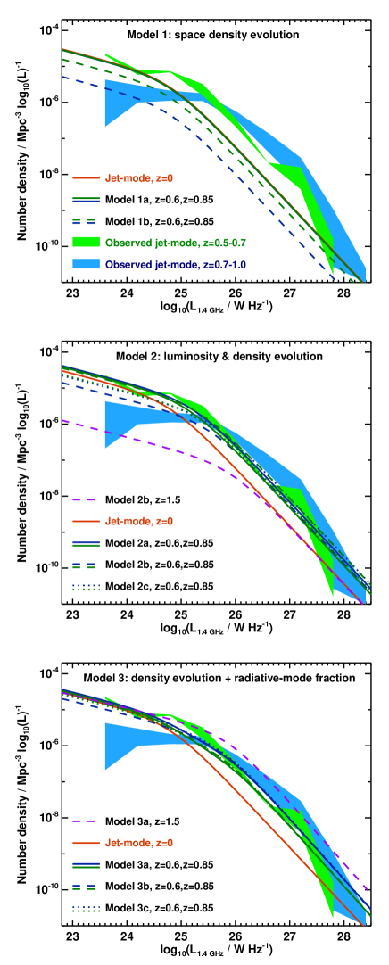
Figure 7: A comparison of the observed jet-mode RLFs with model predictions. In all panels the green and blue shaded regions represent the uncertainty on the jet-mode RLFs at $0.5<z<0.7$ and $0.7<z<1.0$ respectively, as shown in Fig. 5, while the various green and blue lines show the model predictions. The top panel shows the results for versions of Model 1 (space density evolution; see §4.3.1 and §4.3.2), the middle panel shows versions of Model 2 (luminosity density evolution; §4.3.3) and the lower panel shows versions of Model 3 (density evolution with radiative-mode contribution; §4.3.4). In all panels the red solid line shows the $z=0$ jet-mode RLF for comparison. The purple dashed lines show extrapolations of Models 2b and 3a to $z=1.5$. Note that in the top panel the solid lines are largely on top of each other.

4.3.2 Delays in the onset of jet-mode AGN activity

A remarkable discovery over the last decade is that massive galaxies at high redshifts are significantly more compact than those of the same mass in the nearby Universe (e.g. Daddi et al., 2005). However, the host galaxies of powerful radio sources at moderate to high redshifts are as large as those nearby (e.g. Best et al., 1998). Lower power radio-AGN are also found to be hosted by galaxies that are larger than other ellipticals of the same mass (Caldwell et al. in prep.). A plausible explanation is that after massive galaxies have their star-formation quenched there is a time-delay before the surrounding hot halo has established itself into a state where gas cooling and AGN fuelling can proceed, and that this time delay is long enough for the processes that ‘puff up’ the galaxy to have occurred. For example, if the transition to a quenched state is driven by a powerful quasar outburst removing most of the cold gas from the galaxy, then that same outburst might disturb the surrounding hot gas and lead to a delay before gas cooling established. The cooling time of gas at $\approx 10$ kpc radii in massive elliptical galaxies is typically of order a Gyr (e.g. Panagoulia et al., 2014), which interestingly is broadly similar to the timescale for the ‘puffing up’ of a galaxy in the quasar feedback model of Fan et al. (2008), where the removal of gas is argued to induce an expansion of the stellar distribution over a few tens of dynamical times ($\approx 2$ Gyr). Other mechanisms for increasing the sizes of galaxies (e.g. multiple minor mergers) may work on similar timescales.

In order to account for this possibility, Model 1a was adapted to include a time delay $\tau=2$ Gyr between the formation of quiescent galaxies and their ability to produce jet-mode radio-AGN. (Note that in later models, $\tau$ is allowed to be a free parameter; however in this first simple model, the fit to the data is sufficiently poor that meaningless results are obtained, so the 2 Gyr value is used solely for illustrative purposes). In practice this time delay was incorporated by considering the space density of jet-mode radio-AGN at redshift $z$ to evolve as the space density of potential jet-mode host galaxies (from Figure 6) at redshift $z^{\prime}$, where redshift $z^{\prime}$ is the redshift at which the Universe was $\tau$ younger than at redshift $z$. This prediction is shown as Model 1b in Figure 7.

4.3.3 Luminosity-density evolution of jet-mode AGN

These pure density evolution models are clearly unable to explain the behaviour at high radio luminosities, where the space density of jet-mode AGN increases with increasing redshift. This problem may be resolved if the radio luminosities of the sources systematically increase with redshift. Physically, this can be understood as follows. For a given jet-power, the synchrotron luminosity of a source depends strongly on the density of the environment into which it is expanding: in higher density environments the radio lobes remain more confined and adiabatic expansion losses are lower, leading to higher synchrotron luminosities (e.g. Barthel & Arnaud, 1996). At higher redshifts the average density of the Universe is higher, and also the gas fraction is higher. Each of these could plausibly lead to an increase in the radio luminosity with redshift. In Model 2, therefore, the characteristic luminosity ($L_{0}$) of the RLF is allowed to evolve as $(1+z)^{\delta}$, with $\delta$ a free parameter. Model variations 2a, 2b and 2c are considered. In Model 2a, this luminosity evolution is combined with the space density evolution of potential host galaxies at that redshift, as in Model 1a. In Model 2b, the luminosity evolution is combined with the space density evolution of potential hosts, including the time-lag of Model 1b, but allowing the time lag $\tau$ to be a free parameter. In Model 2c, the luminosity evolution is combined with a simple parameterised space density evolution of $\rho_{0}\propto(1+z)^{\eta}$, with $\eta$ a free parameter.

To derive the best-fitting values of the parameters of these models, the maximum likelihood analysis described in Section 4.1 was used, again with 1000 Monte-Carlo iterations for the inclusion or exclusion of unclassified sources. The best-fitting values of each parameter, and their uncertainties, are shown in Table 5. The resultant model predictions for the evolution of the jet-mode RLFs are shown in Figure 7.

Table 5: Best-fit parameter values, and their uncertainties, for the modelling of the jet-mode radio-AGN RLF. The space density of the RLF at redshift $z$ is modelled as declining either with the available space density of potential hosts at redshift $z$ (version ‘a’; §4.3.1), or as the space density of potential hosts at an earlier redshift $z^{\prime}$, where $z^{\prime}$ is the redshift corresponding to a time $\tau$ before redshift $z$ (version ‘b’; §4.3.2), or declining as $(1+z)^{\delta}$ (version ‘c’). In versions of Model 2, the characteristic luminosity of the RLF also evolves as $(1+z)^{\eta}$ (§4.3.3). In versions of Model 3 there is instead an additional contribution from radiative-mode AGN hosts, modelled as the radiative-mode RLF at that redshift scaled up by factors $f_{\rho}$ in space density and $f_{\rm L}$ in luminosity (§4.3.4).

Model	Space density	$\delta$	$\tau$	$\eta$	$f_{\rho}$	$f_{\rm L}$
	evolution		[Gyr]
Model 1a	As potential hosts	—	—	—	—	—
Model 1b	As potential hosts, with delay	—	2.0 (fixed)	—	—	—
Model 2a	As potential hosts	—	—	$1.6\pm 0.2$	—	—
Model 2b	As potential hosts, with delay	—	$1.5\pm 0.2$	$2.8\pm 0.2$	—	—
Model 2c	$\rho_{0}\propto(1+z)^{\delta}$	$-1.6\pm 0.3$	—	$2.8\pm 0.3$	—	—
Model 3a	As potential hosts	—	—	—	$1.2\pm 0.4$	$0.18\pm 0.04$
Model 3b	As potential hosts, with delay	—	$1.4\pm 0.3$	—	$2.0\pm 0.7$	$0.14\pm 0.03$
Model 3c	$\rho_{0}\propto(1+z)^{\delta}$	$-0.9\pm 0.5$	—	—	$2.0\pm 0.8$	$0.14\pm 0.04$

4.3.4 A radiative-mode contribution to the jet-mode AGN

An alternative explanation can also be considered for the short-comings of Model 1 at high radio luminosities. At high radio luminosities the overall RLF is dominated by the radiative-mode sources. It is possible that a subset of the sources classified as jet-mode sources are not truly quiescent galaxies fuelled by cooling of gas within hot gas haloes, but rather are related to the radiative-mode radio-AGN population. At the simplest level this could be due to mis-classification of some sources, although this would require significant cosmic evolution in the EW_[OIII] division line between the populations. More plausible, this could be to do with the physical properties of a ‘jet-mode’ source.

BH12 argued that the distinction between radiative-mode and jet-mode activity was primarily down to the Eddington-scaled accretion rate on to the black hole: for Eddington-scaled accretion rates above about 1%, a geometrically-thin, luminous accretion disk forms and the AGN is classified as radiative-mode; at lower Eddington-scaled accretion rates there is instead a geometrically-thick radiatively-inefficient accretion flow in which the energetic output of the AGN is primarily in the form of powerful radio jets – a jet-mode source. AGN powered by the cooling of gas from hot haloes will invariably be fuelled at relatively low accretion rates and thus will be jet-mode sources. Sources fuelled by cold dense gas are capable of much higher Eddington-scaled accretion rates and therefore can appear as radiative-mode AGN. However, accretion onto the AGN is a stochastic process and it would be unsurprising if at some times cold-gas fuelling occurred at rates below the critical Eddington fraction, leading to a changed accretion mode and a jet-mode classification.

In the nearby Universe the jet-mode radio-AGN population is dominated by the hot-gas fuelled sources (cf. BH12). Thus, the “jet-mode versus radiative-mode” and “hot-gas-fuelled versus cold-gas-fuelled” distinctions are largely synonymous. Towards higher redshifts, however, the prevalence of hot-gas fuelled sources will fall (due to fewer potential hosts) and that of cold-gas fuelled sources rises (due to higher gas availability) and so cold-gas-fuelled sources may begin to make a significant contribution to the jet-mode population. In this respect it is interesting that Janssen et al. (2012) found that high power jet-mode AGN are more likely to be blue in colour, i.e. star forming, which would fit this picture.

To characterise this in a simple manner, the high-redshift jet-mode RLF can be modelled as being composed of two populations. The first population is the genuine hot-gas-fuelled sources and is constructed by evolving the local jet-mode RLF with pure density evolution due to the decreasing space density of potential host galaxies (evolving with variants a, b and c, as for Model 2 above). To this is added a radiative-mode contribution, which is modelled as being the radiative-mode RLF at the relevant redshift, scaled in space density by a factor $f_{\rho}$ and in luminosity by a factor $f_{\rm L}$. The luminosity scaling accounts for the accretion rates being lower at the times that these galaxies are classified as jet-mode. The density scaling factor accounts both for the fact that not all radiative-mode AGN host galaxies may go through jet-mode phases, and for the relative durations of radiative-mode and jet-mode radio phases. Note that $f_{\rho}$ is allowed to be greater than unity, if the jet-mode phase is longer lived.

Once again, Monte-Carlo iterations of the maximum likelihood analysis were employed to derive the best-fit parameters for these models, Models 3a, 3b and 3c. The best-fitting values of each parameter are shown in Table 5 and the model predictions are shown in Figure 7.

5 Discussion

5.1 Radiative-mode radio-AGN

The evolution in the space density of radiative-mode radio-AGN (a factor $\sim 7$ from the local Universe to $z\sim 0.75$) is remarkably similar to the amount by which the cosmic star formation rate density has increased over the same cosmic interval (e.g. Sobral et al., 2013; Madau & Dickinson, 2014, and references therein). It is also comparable to the evolution of the quasar luminosity function (ie. radio-quiet radiative-mode AGN; Hasinger et al., 2005; Hopkins et al., 2007; Croom et al., 2009), although a combination of density and luminosity evolution is usually preferred for the latter. These results are consistent with the picture whereby both the radiative-mode AGN and star-formation activity are simply controlled by the availability of a supply of cold gas to the galaxy (e.g. see discussion in Heckman & Best, 2014).

5.2 The jet-mode RLF

At low radio luminosities ($L_{\rm 1.4GHz}<10^{25}$W Hz^-1) the jet-mode RLF shows a gradual decline with increasing redshift, which can be explained by a decrease in the space density of available host galaxies (Model 1). Thus, previous analyses of the prevalence of radio-AGN as a function of stellar mass out to $z\sim 1$ (Tasse et al., 2008; Donoso et al., 2009; Simpson et al., 2013), which have been dominated by sources at these luminosities, have found results broadly in line with those of the local Universe.

At high radio luminosities, however, an increase in space density with increasing redshift is seen. The results of Figure 7 indicate that variants of both Models 2 and 3 are able to account for this, although Model 2 does so with one fewer free parameter. Amongst the Model 2 options, Model 2b provides the best match to the observed data. This luminosity-density evolution model requires the jet-mode AGN luminosities to scale as $(1+z)^{2.8}$ and adopts a 1.5 Gyr delay between the creation of a quiescent galaxy and the onset of jet-mode radio-AGN activity due to the cooling of hot gas from the halo. It is interesting that this time delay is in line with the typical cooling time of gas at $\approx 10$ kpc radii in massive elliptical galaxies (e.g. Panagoulia et al., 2014) which might provide the AGN fuel source, and also with the $\approx 2$ Gyr dynamical expansion timescale calculated in the quasar-feedback model of Fan et al. (2008).

There is little to distinguish between the various Model 3 options. Each predicts $f_{\rm L}\approx$ 0.1-0.2 implying that, if this model is correct, cold-gas-fuelled AGN scale down in luminosity by nearly an order of magnitude (due to a corresponding decrease in accretion rate) as they transition from radiative-mode to jet-mode AGN activity. This value makes sense physically, as it is the decrease required to take a radiative-mode AGN (typical $L/L_{\rm Edd}\sim 0.1$) down into the advection-dominated accretion flow regime ($L/L_{\rm Edd}\mathrel{\hbox to0.0pt{\lower 3.0pt\hbox{$\mathchar 536\relax$}\hss}\raise 2.0pt\hbox{$\mathchar 316\relax$}}0.01$). Each model also predicts $f_{\rho}\approx$ 1-2, implying that the two accretion rate regimes would be active for similar fractions of time.

It is impossible with the current data to distinguish which, if either, of these two explanations is correct for the evolution of the jet-mode RLF. However, extending this analysis to still higher redshift would lead to a clear distinction between the two. The purple dotted lines on the middle and lower panels of Figure 7 demonstrate the predictions of Models 2b and 3a for the RLF of jet-mode radio-AGN at redshift $z=1.5$, and these differ by an order of magnitude at most radio luminosities. Extending the analysis of this paper to higher redshifts is therefore critical, albeit that this will require near-infrared spectroscopy if source classification is to be consistently carried out using the oxygen lines.

5.3 Evolution of the jet-mode AGN heating rate

It is interesting to consider the implications of these results for the importance of AGN-feedback as a function of redshift. As described by Heckman & Best (2014) and references therein, radio luminosity can be broadly converted into a jet mechanical luminosity as

$$P_{\rm mech}=7\times 10^{36}f_{\rm cav}\left(\frac{L_{\rm 1.4GHz}}{10^{25}{\rm WHz}^{-1}}\right)^{0.68}\,{\rm W}$$

where $f_{\rm cav}\approx 4$ relates the work done in inflating the radio lobes to their pressure and volume, $E_{\rm cav}=f_{\rm cav}pV$. If this relation remains invariant with redshift (which is not necessarily the case if radio luminosities are boosted at higher redshifts by higher confining gas densities) then by combining this relationship with the RLF, the heating rate function as a function of radio luminosity can be derived. This is shown for jet-mode radio-AGN in the top panel of Figure 8, as calculated from the broken power-law fits to the RLF at each of the three redshifts. As can be seen, locally the majority of heating arises from relatively low luminosity sources, but at higher redshift the peak moves out to the higher luminosity population. The overall heating rate per unit volume is found by integrating this curve and is shown, relative to the local value, in the lower panel of Figure 8: it rises out to $z\sim 0.5$ but then falls again. The predictions of the various models from Section 4.3 are also shown on this plot. For comparison, the evolution of the cosmic star formation rate density (ie., broadly, the cold gas supply) is also shown, while the evolution of the space density of massive quiescent galaxies (ie., potential jet-mode AGN hosts) broadly follows Model 1a (by definition of that model). Once again it can be seen that Model 2b (luminosity-density evolution with a time-delay) provides the best match to the data, and that the model predictions diverge strongly towards higher redshifts.

These results can also be compared against previous phenomenological models of jet-mode radio-AGN activity. Croton et al. (2006) predicted, in their semi-analytic modelling incorporating radio-AGN feedback, that the accretion rate onto radio AGN should remain relatively flat out to $z\sim 1.5$ and then fall by an order of magnitude out to $z\approx 4$. Körding et al. (2008) developed a model for the accretion rate function of low-luminosity black holes based on the radio core emission, to predict that the energetic output of jet-mode AGN should rise by a factor 2-3 between $z=0$ and $z=0.5$, and then remain broadly flat out to $z=3$. Merloni & Heinz (2008) similarly used an AGN synthesis model to predict that the kinetic energy output of jet-mode radio-AGN (their ‘LK’ population) should be flat or shallowly rising out to $z\approx 1$ and then gradually fall thereafter. Mocz et al. (2013) combined this AGN population model with a parameterisation of the evolution of the accretion rates on to black holes, to make a very similar prediction for the LK population. All of these predictions are in broad agreement with the data, although none match precisely. Higher accuracy determinations and an extension to higher redshift would allow a more critical test of these models.

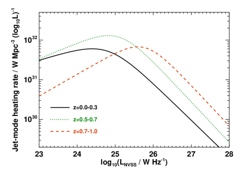
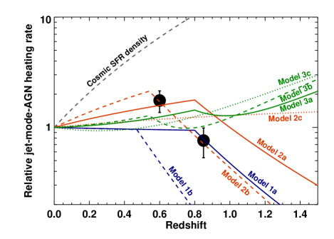
Figure 8: Top: the heating rate function of jet-mode radio-AGN over three redshift ranges, assuming that the relationship between radio luminosity and jet mechanical energy derived locally still holds at higher redshift. Bottom: the total integrated heating rate of jet-mode radio-AGN at redshifts $0.5<z<0.7$ and $0.7<z<1.0$ compared to the local value. Also shown are the predictions for the evolution from various models described in Section 4.3. For comparison, the evolution of the cosmic star formation rate density is also shown, while the evolution of the space density of massive quiescent galaxies effectively follows Model 1a.

6 Conclusions

This paper presents the first observational measurement of the cosmic evolution of jet-mode radio-AGN feedback out to $z=1$. Eight flux-limited radio source samples with high spectroscopic completeness are combined to produce a catalogue of over 200 radio sources at redshifts $0.5<z<1.0$, which are then spectroscopically classified into jet-mode and radiative-mode AGN classes. By comparison with the large samples of local radio-AGN selected from the Sloan Digital Sky Survey (Best & Heckman, 2012), the cosmic evolution of the RLF of each radio source class is derived independently.

Radiative-mode radio-AGN show a monotonic increase in space density with redshift out to $z=1$, in line with the increasing space density of cosmic star formation. This is consistent with these AGN being fuelled by cold gas. Jet-mode radio-AGN show more complicated behaviour. At low radio luminosities ($L_{\rm 1.4GHz}\mathrel{\hbox to0.0pt{\lower 3.0pt\hbox{$\mathchar 536\relax$}\hss}\raise 2.0pt\hbox{$\mathchar 316\relax$}}10^{24}$W Hz^-1) their space density decreases gradually with increasing redshift. At intermediate luminosities ($10^{24}-10^{26}$W Hz^-1) it rises out to $z\approx 0.5$ and then falls at higher redshift. At the highest radio luminosities the space density continues to increase out to $z=1$.

Simple models are developed to explain the observed evolution. The characteristic space density of jet-mode AGN is modelled as decreasing with redshift in accordance with the number of massive quiescent galaxies, in which they are believed to be hosted. A time delay between the formation of the quiescent galaxy and its availability as a jet-mode radio-AGN host is allowed, in case there is a lag between the quenching of star formation activity and the onset of the hot gas cooling flows in the galaxy which fuel the jet-mode AGN. The best-fitting models prefer a time delay of 1.5–2 Gyr which, intriguingly, is in line with the typical cooling time of hot gas at radii of $\approx 10$ kpc around massive ellipticals.

The evolution at higher radio luminosities can be accounted for either by allowing for evolution of the characteristic luminosity of the jet-mode RLF with redshift (roughly as $(1+z)^{3}$) or if the jet-mode radio-AGN population also includes some contribution of cold-gas-fuelled sources hosted by the typical hosts of radiative-mode AGN, just caught at a time when their accretion rate was low. The current data are unable to distinguish between these two possibilities, but it is shown that extending the analysis to still higher redshifts would provide a very clear diagnostic.

If the relationship between jet mechanical luminosity and radio luminosity remains constant across cosmic time then the results indicate that the volume-averaged energetic output of jet-mode radio-AGN (ie. of radio-AGN feedback) rises gradually out to about $z\sim 0.5$ and then falls beyond that. This is broadly in line with the expectations of semi-analytic and phenomenological models. Extending the analysis to higher redshifts and improving the accuracy with larger radio source samples would provide a more critical test of these models.

Appendix A The radio source sample data

Table 6: The properties of the 211-source combined sample used in the analysis of this paper.

Source	S1.4GHz	Redshift	Type	Spec.	log10(L)	Classification
	(Jy)		of z	Index	(W Hz-1)
WP85:
0538+49	21.79	0.545	S	0.77	28.38	Radiative-mode
1828+48	16.69	0.692	S	0.78	28.49	Quasar (radiative-mode)
1328+30	14.70	0.850	S	0.53	28.59	Quasar (radiative-mode)
0809+48	14.37	0.871	S	0.94	28.71	Quasar (radiative-mode)
0407-65	13.47	0.962	S	1.11	28.84	Radiative-mode
0518+16	12.99	0.759	S	0.92	28.52	Quasar (radiative-mode)
0409-75	12.72	0.693	S	0.86	28.40	Radiative-mode
1458+71	8.89	0.905	S	0.77	28.49	Radiative-mode
0316+16	8.01	0.907	S	0.79	28.46	Radiative-mode
2032-35	7.62	0.631	S	1.10	28.13	Radiative-mode
1005+07	6.62	0.877	S	0.97	28.39	Radiative-mode
0252-71	6.55	0.568	S	1.14	27.96	Radiative-mode
1157+73	6.41	0.97	S	0.70	28.40	Radiative-mode
1609+66	6.19	0.550	S	0.76	27.83	Radiative-mode
0404+76	6.01	0.599	S	0.60	27.87	Radiative-mode
1254+47	5.59	0.996	S	1.02	28.47	Radiative-mode
1634+62	5.09	0.988	S	0.96	28.40	Quasar (radiative-mode)
1526-42	5.08	0.5	P	1.02	27.69	Unclassified
0117-15	4.91	0.565	S	0.90	27.78	Radiative-mode
2128+04	4.84	0.99	S	0.67	28.29	Unclassified
2331-41	4.84	0.907	S	0.91	28.27	Radiative-mode
0022-42	4.71	0.937	S	0.77	28.26	Radiative-mode
1453-10	4.6	0.938	S	0.93	28.29	Quasar (radiative-mode)
1637+62	4.45	0.750	S	1.03	28.07	Radiative-mode
2342+82	4.35	0.735	S	0.95	28.01	Quasar (radiative-mode)
1136-13	4.29	0.556	S	0.65	27.65	Quasar (radiative-mode)
0235-19	4.27	0.620	S	0.87	27.81	Radiative-mode
2135-20	4.27	0.636	S	0.82	27.83	Radiative-mode
0157-31	4.03	0.677	S	0.81	27.87	Quasar (radiative-mode)
CoNFIG:
3C216	4.23	0.67	S	0.77	27.87	Quasar (radiative-mode)
3C228	3.71	0.552	S	0.84	27.63	Radiative-mode
3C225	3.34	0.58	S	1.01	27.66	Radiative-mode
3C337	3.16	0.63	S	0.67	27.65	Radiative-mode
3C254	3.13	0.736	S	0.92	27.87	Quasar (radiative-mode)
4C-06.35	2.96	0.625	S	0.88	27.66	Quasar (radiative-mode)
3C275.1	2.90	0.557	S	0.91	27.54	Quasar (radiative-mode)
3C265	2.89	0.811	S	0.94	27.94	Radiative-mode
3C247	2.88	0.749	S	0.84	27.83	Radiative-mode
4C03.18	2.71	0.535	S	0.52	27.40	Radiative-mode
3C207	2.61	0.680	S	0.81	27.68	Quasar (radiative-mode)
3C336	2.61	0.927	S	0.73	27.98	Quasar (radiative-mode)
3C340	2.60	0.775	S	0.68	27.78	Radiative-mode
4C19.44	2.59	0.72	S	0.53	27.67	Quasar (radiative-mode)
4C33.21	2.47	0.603	S	0.56	27.48	Radiative-mode
4C01.39	2.40	0.819	S	0.70	27.81	Radiative-mode
3C289	2.40	0.967	S	0.79	28.00	Radiative-mode
3C226	2.39	0.818	S	0.93	27.86	Radiative-mode
4C01.42	2.26	0.792	S	0.66	27.74	Radiative-mode
4C37.24	2.26	0.919	S	0.65	27.88	Quasar (radiative-mode)
4C59.16	2.18	0.961	S	0.56	27.88	Radiative-mode
3C217	2.09	0.898	S	0.95	27.91	Radiative-mode
3C334	1.99	0.555	S	0.84	27.36	Quasar (radiative-mode)
3C277.2	1.95	0.766	S	0.89	27.70	Radiative-mode
1355+01	1.92	0.797	S	0.70	27.68	Radiative-mode
3C202	1.88	0.809	S	0.72	27.69	Radiative-mode
3C352	1.87	0.806	S	0.90	27.73	Radiative-mode
4C20.33	1.81	0.871	S	0.70	27.75	Quasar (radiative-mode)
4C13.56	1.81	0.672	S	0.65	27.47	Radiative-mode
4C54.25	1.74	0.716	S	0.56	27.50	Unclassified

Table 6: continued

Source	S1.4GHz	Redshift	Type	Spec.	log10(L)	Classification
	(Jy)		of z	Index	(W Hz-1)
CoNFIG (cont.):
4C53.18	1.60	0.869	S	0.77	27.71	Unclassified
4C17.56	1.57	0.777	S	0.62	27.55	Radiative-mode
4C43.22	1.57	0.572	S	0.70	27.26	Radiative-mode
4C24.31	1.56	0.653	S	0.78	27.41	Quasar (radiative-mode)
4C17.48	1.53	0.521	S	0.74	27.16	Radiative-mode
4C04.40	1.50	0.531	S	0.83	27.19	Jet-mode
3C288.1	1.49	0.964	S	0.88	27.82	Quasar (radiative-mode)
4C-00.50	1.47	0.892	S	0.56	27.64	Quasar (radiative-mode)
4C46.21	1.44	0.527	S	0.72	27.14	Radiative-mode
3C344	1.42	0.52	S	0.88	27.15	Unclassified
4C61.34	1.35	0.523	S	0.67	27.10	Quasar (radiative-mode)
3C272	1.35	0.944	S	0.98	27.78	Radiative-mode
3C323	1.34	0.679	S	0.91	27.41	Radiative-mode
3C342	1.34	0.561	S	0.81	27.19	Quasar (radiative-mode)
4C51.25	1.31	0.561	S	0.81	27.18	Radiative-mode
4C20.29	1.27	0.68	S	0.66	27.33	Quasar (radiative-mode)
4C32.34	1.26	0.564	S	0.98	27.21	Radiative-mode
3C232	1.25	0.531	S	0.79	27.10	Quasar (radiative-mode)
4C46.25	1.16	0.743	S	0.71	27.39	Unclassified
3C261	1.15	0.613	S	1.00	27.26	Quasar (radiative-mode)
3C281	1.12	0.599	S	0.87	27.20	Quasar (radiative-mode)
4C59.11	1.08	0.707	S	0.88	27.35	Radiative-mode
4C00.35	1.08	0.746	S	0.71	27.37	Radiative-mode
4C15.34	1.07	0.97	P	0.72	27.64	Unclassified
4C17.49	1.06	0.51	P	0.90	27.01	Jet-mode
4C17.54	1.01	0.675	S	0.68	27.23	Radiative-mode
3C248	0.99	0.83	P	1.05	27.53	Unclassified
4C49.21	0.96	0.73	P	0.93	27.35	Unclassified
4C-02.43	0.96	0.70	P	0.81	27.28	Unclassified
4C00.34	0.92	0.906	S	0.94	27.56	Quasar (radiative-mode)
3C251	0.92	0.781	S	0.89	27.39	Quasar (radiative-mode)
1300+585	0.90	0.80	P	0.51	27.30	Unclassified
4C25.36	0.88	0.98	P	0.81	27.59	Unclassified
4C10.33	0.88	0.540	S	0.88	26.98	Quasar (radiative-mode)
4C16.30	0.87	0.630	S	0.60	27.08	Quasar (radiative-mode)
4C43.19	0.85	0.81	P	0.96	27.41	Jet-mode
4C09.39	0.81	0.696	S	0.59	27.14	Quasar (radiative-mode)
1229-013	0.81	0.59	P	0.68	27.00	Unclassified
4C31.40	0.81	0.828	S	1.06	27.44	Radiative-mode
Parkes:
2154-184	2.39	0.668	S	1.17	27.70	Quasar (radiative-mode)
0222-008	1.11	0.687	S	0.79	27.31	Quasar (radiative-mode)
2355-010	0.83	0.76	P	1.02	27.35	Unclassified
0059+017	0.80	0.692	S	1.06	27.24	Radiative-mode
1336+020	0.74	0.567	S	1.02	26.99	Radiative-mode
2159-201	0.60	0.75	P	1.66	27.35	Unclassified
2158-177	0.54	0.81	P	0.93	27.21	Unclassified
0242+028	0.53	0.767	S	0.95	27.15	Radiative-mode
0043+000	0.53	0.60	P	1.03	26.90	Unclassified
7CRS:
1732+6535	0.73	0.856	S	0.98	27.41	Quasar (radiative-mode)
5C6.19	0.44	0.799	S	0.80	27.07	Radiative-mode
0221+3417	0.44	0.852	S	0.87	27.15	Unclassified
1816+6710	0.40	0.92	S	0.95	27.21	Jet-mode
5C7.111	0.37	0.628	S	0.77	26.74	Radiative-mode
1807+6831	0.37	0.58	S	0.79	26.66	Radiative-mode
5C7.8	0.30	0.673	S	0.89	26.75	Radiative-mode
1755+6830	0.28	0.744	S	0.85	26.81	Radiative-mode
5C7.85	0.27	0.995	S	0.78	27.08	Quasar (radiative-mode)
5C7.205	0.26	0.710	S	0.88	26.74	Radiative-mode

Table 6: continued

Source	S1.4GHz	Redshift	Type	Spec.	log10(L)	Classification
	(Jy)		of z	Index	(W Hz-1)
7CRS (cont.):
5C7.118	0.25	0.527	S	0.71	26.39	Radiative-mode
1819+6550	0.23	0.724	S	0.83	26.70	Quasar (radiative-mode)
1758+6535	0.23	0.80	S	0.78	26.79	Radiative-mode
1826+6510	0.22	0.646	S	0.94	26.59	Jet-mode
1815+6815	0.19	0.794	S	1.03	26.77	Jet-mode
5C7.25	0.19	0.671	S	0.66	26.50	Radiative-mode
5C6.264	0.19	0.831	S	0.82	26.75	Quasar (radiative-mode)
5C6.258	0.19	0.752	S	0.61	26.59	Unclassified
5C7.125	0.19	0.801	S	0.63	26.65	Radiative-mode
1816+6605	0.18	0.92	S	0.95	26.87	Unclassified
5C6.233	0.18	0.560	S	0.95	26.34	Radiative-mode
TOOT:
TOOT00_1200	0.27	0.691	S	0.79	26.71	Radiative-mode
TOOT00_1034	0.14	0.580	S	0.66	26.22	Jet-mode
TOOT00_1140	0.12	0.911	S	0.66	26.61	Jet-mode
TOOT00_1072	0.11	0.577	S	0.72	26.12	Unclassified
TOOT00_1267	0.100	0.968	S	0.74	26.61	Radiative-mode
TOOT00_1235	0.099	0.743	S	0.55	26.29	Quasar (radiative-mode)
TOOT00_1255	0.034	0.582	S	0.60	25.59	Unclassified
CENSORS:
CEN-6	0.24	0.547	S	0.54	26.37	Radiative-mode
CEN-12	0.070	0.821	S	0.95	26.34	Radiative-mode
CEN-17	0.062	0.893	S	0.73	26.31	Unclassified
CEN-22	0.053	0.928	S	0.95	26.35	Radiative-mode
CEN-29	0.038	0.965	S	0.80	26.20	Radiative-mode
CEN-37	0.032	0.511	S	0.76	25.47	Unclassified
CEN-43	0.026	0.778	S	0.65	25.78	Unclassified
CEN-45	0.026	0.796	S	0.89	25.85	Jet-mode
CEN-47	0.025	0.508	S	0.81	25.37	Radiative-mode
CEN-55	0.021	0.557	S	0.65	25.36	Jet-mode
CEN-62	0.018	0.574	S	0.63	25.32	Jet-mode
CEN-65	0.018	0.549	S	0.58	25.25	Jet-mode
CEN-70	0.017	0.645	S	0.94	25.47	Radiative-mode
CEN-74	0.016	0.667	S	0.92	25.47	Radiative-mode
CEN-83	0.014	0.521	S	0.98	25.15	Radiative-mode
CEN-86	0.013	0.82	P	0.62	25.53	Unclassified
CEN-89	0.013	0.909	S	1.00	25.73	Unclassified
CEN-92	0.013	0.743	S	1.27	25.57	Radiative-mode
CEN-104	0.011	0.88	P	1.19	25.67	Jet-mode
CEN-107	0.010	0.512	S	0.82	24.99	Jet-mode
CEN-109	0.010	0.72	P	0.91	25.35	Jet-mode
CEN-113	0.0097	0.94	P	1.23	25.71	Jet-mode
CEN-115	0.0096	0.545	S	1.20	25.09	Jet-mode
CEN-125	0.0084	0.701	S	1.02	25.27	Jet-mode
CEN-127	0.0083	0.922	S	1.23	25.61	Unclassified
CEN-136	0.0075	0.629	S	1.08	25.11	Unclassified
CEN-137	0.0074	0.526	S	0.93	24.89	Jet-mode
CEN-138	0.015	0.508	S	0.71	25.11	Unclassified
Hercules:
53W008	0.31	0.736	S	0.79	26.83	Radiative-mode
53W031	0.12	0.627	S	0.70	26.22	Radiative-mode
53W023	0.11	0.569	S	0.87	26.13	Jet-mode
53W046	0.063	0.528	S	0.69	25.78	Radiative-mode
53W080	0.028	0.542	S	0.80	25.47	Quasar (radiative-mode)
53W047	0.024	0.532	S	0.67	25.36	Jet-mode
53W067	0.023	0.759	S	0.81	25.74	Jet-mode
53W026	0.021	0.550	S	0.74	25.36	Jet-mode
53W048	0.012	0.676	S	0.81	25.32	Jet-mode
53W060	0.010	0.62	P	0.93	25.18	Unclassified

Table 6: continued

Source	S1.4GHz	Redshift	Type	Spec.	log10(L)	Classification
	(Jy)		of z	Index	(W Hz-1)
Hercules (cont.):
53W041	0.0094	0.59	P	0.88	25.10	Unclassified
53W077	0.0078	0.786	S	0.87	25.32	Jet-mode
53W005	0.0076	0.765	S	1.09	25.33	Unclassified
53W019	0.0068	0.542	S	0.72	24.85	Jet-mode
53W083	0.0050	0.628	S	0.70	24.86	Jet-mode
53W089	0.0025	0.635	S	1.29	24.69	Jet-mode
SXDF:
VLA0001	0.080	0.627	S	—	26.08	Radiative-mode
VLA0011	0.0080	0.645	S	—	25.11	Jet-mode
VLA0012	0.0066	0.865	S	—	25.33	Unclassified
VLA0018	0.0048	0.919	S	—	25.26	Jet-mode
VLA0019	0.0048	0.695	S	—	24.97	Unclassified
VLA0023	0.0042	0.586	S	—	24.73	Radiative-mode
VLA0024	0.0036	0.516	S	—	24.54	Jet-mode
VLA0025	0.0032	0.963	S	—	25.13	Quasar (radiative-mode)
VLA0028	0.0028	0.632	S	—	24.63	Jet-mode
VLA0030	0.0026	0.535	S	—	24.42	Jet-mode
VLA0033	0.0024	0.647	S	—	24.58	Jet-mode
VLA0036	0.0021	0.872	S	—	24.84	Jet-mode
VLA0039	0.0018	0.89	P	—	24.78	Jet-mode
VLA0045	0.0015	0.553	S	—	24.23	Jet-mode
VLA0060	0.0010	0.881	S	—	24.53	Unclassified
VLA0061	0.00099	0.668	S	—	24.24	Radiative-mode
VLA0064	0.00097	0.515	S	—	23.97	Unclassified
VLA0067	0.00085	0.649	S	—	24.14	Jet-mode
VLA0080	0.00072	0.99	P	—	24.46	Jet-mode
VLA0083	0.00071	0.94	P	—	24.47	Unclassified
VLA0108	0.00050	0.627	S	—	23.88	Jet-mode
VLA0115	0.00047	0.88	P	—	24.20	Unclassified
VLA0120	0.00044	0.843	S	—	24.13	Radiative-mode
VLA0145	0.00035	0.547	S	—	23.58	Jet-mode
VLA0148	0.00034	0.64	P	—	23.73	Unclassified
VLA0151	0.00034	0.579	S	—	23.63	Jet-mode
VLA0169	0.00030	0.553	S	—	23.53	Jet-mode
VLA0177	0.00029	0.515	S	—	23.44	Jet-mode
VLA0186	0.00028	0.567	S	—	23.51	Jet-mode
VLA0202	0.00025	0.83	P	—	23.87	Unclassified
VLA0209	0.00025	0.76	P	—	23.75	Unclassified
VLA0217	0.00024	0.643	S	—	23.57	Jet-mode

Table 6 provides data for the sources within the eight samples used for this study. The 1.4 GHz flux density limits and sky area coverage of each sample are given in Table 1. Redshifts are selected to be between 0.5 and 1.0; where a spectroscopic redshift does not exist then a photometric redshift (in some cases based only on the K$-z$ relation) is used instead. These are indicated in the table. Readers should refer back to the papers originally presenting the samples (as described in Section 2) for details of the origins of the redshifts and other source properties. Spectral indices are calculated at 1.4 GHz, following Ker et al. (2012), although the effect of any spectral curvature on the calculated radio luminosities is negligible at these redshifts. No spectral indices are available for the SXDF sources, so a value of $\alpha=0.75$ is assumed. Classifications into jet-mode and radiative-mode are described in Section 3.

Appendix B New observational results

Spectroscopic observations were carried out of a subsample of the galaxies which either lacked a spectroscopic redshift or for which no suitable spectrum was available for classification. These observations were carried out during two runs on the William Herschel Telescope (WHT) from 22-24 May and 18-19 October 2012 (the latter of which was almost entirely lost to bad weather), with further observations obtained in service mode in November 2012. Observations were carried out using the duel–beam ISIS spectrograph, with the 5300Å dichroic, the R300B and R158R gratings in the blue and red arms respectively, and a 1.5 arcsec slit. Combined, these provided a usable wavelength coverage from $\approx 3500$Å to $\approx 9500$Å, and a spectral resolution of about 15Å.

Target exposure times varied according to the flux expected for emission lines if the source was of radiative-mode class (for which emission line flux correlates broadly with radio flux density). Initial integrations were analysed in real-time (except for the service mode observations), and observations were repeated if no classification was available, up to a maximum of 40 mins. Data reduction was carried out in IRAF using standard procedures, with internal calibration lamps used for flat-fielding and wavelength calibration. Spectrophotometric calibration was carried out using the standard star HZ21 for the May run and G191-B2B in October and November.

Table 7: Redshifts and emission line properties of sources in the sample which were observed in the new WHT observations.

Source	Observation	Exposure	Redshift	$f_{\rm[OII]}$	$f_{\rm[OIII]}$	$EW_{\rm[OII]}$	$EW_{\rm[OIII]}$	Class
	date	time / s		[$10^{-19}$W m-2]		Å	Å
4C33.21	2012-10-19	540	0.603	26.1	53	95	125	Radiative-mode
4C59.16	2012-05-24	1200	0.961	13.4	13.1	22	22	Radiative-mode
1355+01	2012-05-23	1200	0.797	35.0	90	63	88	Radiative-mode
3C202	2012-10-19	420	0.809	16.2	95	80	250	Radiative-mode
4C13.56	2012-05-24	1200	0.672	4.7		16		Unclassified
4C54.25	2012-05-23	1200	0.716	2.9		11		Unclassified
4C53.18	2012-05-22	1200	0.869	1.0		6		Unclassified
4C17.56	2012-05-24	1800	0.777	4.1	4.5	21	10	Radiative-mode
4C17.48	2012-05-24	1200	0.521	4.9	25.0	16	48	Radiative-mode
4C04.40	2012-05-24	1200	0.531					Jet-mode
4C46.21	2012-05-23	1200	0.527	38.8	68.8	45	44	Radiative-mode
4C51.25	2012-05-23	1200	0.561	5.4	22.3	10	18	Radiative-mode
4C32.34	2012-05-23	1200	0.564	59.1	402	80	275	Radiative-mode
4C59.11	2012-05-23	1200	0.707		72.4		15	Radiative-mode
4C00.35	2012-05-23	1200	0.746	13.1	12.6	19	10	Radiative-mode
4C17.54	2012-05-24	1200	0.675	14.1	14.5	80	44	Radiative-mode
4C43.19	2012-10-19	1200						Jet-mode
PKS0059+017	2012-11-10	900	0.692	6.5	10.6	250	200	Radiative-mode
PKS1336+020	2012-05-23	1200	0.567	32.3	336	28	166	Radiative-mode
53W008	2012-05-22	2400	0.736	3.2	8.8	7	13	Radiative-mode
53W031	2012-05-22	2400	0.627	0.97	1.65	8	5	Radiative-mode
53W023	2012-05-22	2400	0.569					Jet-mode
53W080	2012-05-22	2400	0.542	12.3	36.1	7	23	Radiative-mode
53W047	2012-05-22	2400	0.532					Jet-mode
53W077	2012-05-23	2400	0.786					Jet-mode
53W005	2012-05-23	2400	0.765	3.7		13		Unclassified

Table 8: Redshifts and emission line properties for sources observed with the WHT that were initially within the sample based on their photometric redshifts, but excluded from analysis on the basis of their new spectroscopic redshifts (or, for PKS1329+012 and PKS0045-009, due to the final flux density limit applied to the Parkes sample).

Source	Observation	Exposure	Redshift	$f_{\rm[OII]}$	$f_{\rm[OIII]}$	$EW_{\rm[OII]}$	$EW_{\rm[OIII]}$
	date	time / s		[$10^{-19}$W m-2]		Å	Å
4C16.27	2012-05-24	1200	1.452	3.4		10
1152+551	2012-05-23	1800	1.195	8.1		10
4C29.46	2012-05-24	1200	0.397		177		132
4C12.41	2012-05-24	1200	1.10	10.0		16
4C59.10	2012-05-22	1200	1.245	5.3		45
4C20.28	2012-05-22	1200	0.424	8.2	53.1	42	115
PKS1352+008	2012-05-22	1200	1.167	1.7		12
PKS1337-033	2012-05-24	1200	0.487	1.6	4.9		129
PKS1329+012	2012-05-24	2400	0.873	1.1		10
PKS0045-009	2012-11-10	900	0.832	3.9		120

The properties of the resulting spectra are presented in Table 7 for observed sources that remained within the final sample (equivalent widths are rest-frame values). Table 8 presents the data for sources that were excluded from the final analysis because their spectroscopic redshift lay outside of the range $0.5<z<1.0$ studied here. In addition to these, the source PKS0010+005 was excluded from analysis based on the new WHT observations. This source has a photometric redshift of 0.4, but a spectroscopic redshift of 0.606 is quoted in Dunlop et al. (1989) based on a private communication from Spinrad. However, Spinrad’s spectrum remains unpublished and the WHT data failed to detect emission lines consistent with this redshift (or to determine any other redshift). Therefore the photometric redshift was adopted for PKS0010+005, leading to its exclusion from the sample. Finally, Table 8 includes data for PKS1329+012 and PKS0045-009 which were observed with the WHT but fell below the eventual flux density limit applied to the Parkes subsample.

References

- Appleton et al. (2004) Appleton P. N. et al. 2004, ApJ Supp., pp 147–150
- Baldi & Capetti (2010) Baldi R. D., Capetti A., 2010, A&A, 519, 48
- Baldry et al. (2012) Baldry I. K. et al. 2012, MNRAS, 421, 621
- Barthel & Arnaud (1996) Barthel P. D., Arnaud K. A., 1996, MNRAS, 283, L45
- Becker et al. (1995) Becker R. H., White R. L., Helfand D. J., 1995, ApJ, 450, 559
- Best et al. (2003) Best P. N., Arts J. N., Röttgering H. J. A., Rengelink R., Brookes M. H., Wall J., 2003, MNRAS, 346, 627
- Best & Heckman (2012) Best P. N., Heckman T. M., 2012, MNRAS, 421, 1569
- Best et al. (2006) Best P. N., Kaiser C. R., Heckman T. M., Kauffmann G., 2006, MNRAS, 368, L67
- Best et al. (2005) Best P. N., Kauffmann G., Heckman T. M., Brinchmann J., Charlot S., Ž. Ivezić White S. D. M., 2005, MNRAS, 362, 25
- Best et al. (1998) Best P. N., Longair M. S., Röttgering H. J. A., 1998, MNRAS, 295, 549
- Best et al. (2007) Best P. N., von der Linden A., Kauffmann G., Heckman T. M., Kaiser C. R., 2007, MNRAS, 379, 894
- Böhringer et al. (1993) Böhringer H., Voges W., Fabian A. C., Edge A. C., Neumann D. M., 1993, MNRAS, 264, L25
- Bower et al. (2006) Bower R. G., Benson A. J., Malbon R., Helly J. C., Frenk C. S., Baugh C. M., Cole S., Lacey C. G., 2006, MNRAS, 370, 645
- Brookes et al. (2008) Brookes M. H., Best P. N., Peacock J. A., Röttgering H. J. A., Dunlop J. S., 2008, MNRAS, 385, 1297
- Brookes et al. (2006) Brookes M. H., Best P. N., Rengelink R., Röttgering H. J. A., 2006, MNRAS, 366, 1265
- Burns (1990) Burns J. O., 1990, AJ, 99, 14
- Buttiglione et al. (2010) Buttiglione S., Capetti A., Celotti A., Axon D. J., Chiaberge M., Macchetto F. D., Sparks W. B., 2010, A&A, 509, 6
- Carilli et al. (1994) Carilli C. L., Perley R. A., Harris D. E., 1994, MNRAS, 270, 173
- Cattaneo et al. (2009) Cattaneo A. et al. 2009, Nat, 460, 213
- Cid Fernandes et al. (2010) Cid Fernandes R., Stasińska G., Schlickmann M. S., Mateus A., Vale Asari N., Schoenell W., Sodré L., 2010, MNRAS, 403, 1036
- Cimatti et al. (2013) Cimatti A., Brusa M., Talia M., Mignoli M., Rodighiero G., Kurk J., Cassata P., Halliday C., Renzini A., Daddi E., 2013, ApJ, 779, L13
- Condon (1989) Condon J. J., 1989, ApJ, 338, 13
- Condon et al. (1998) Condon J. J., Cotton W. D., Greisen E. W., Yin Q. F., Perley R. A., Taylor G. B., Broderick J. J., 1998, AJ, 115, 1693
- Croom et al. (2009) Croom S. M. et al. 2009, MNRAS, 399, 1755
- Croton et al. (2006) Croton D. J. et al. 2006, MNRAS, 365, 11
- Daddi et al. (2005) Daddi E. et al. 2005, ApJ, 626, 680
- Domínguez Sánchez et al. (2011) Domínguez Sánchez et al. 2011, MNRAS, 417, 900
- Donoso et al. (2009) Donoso E., Best P. N., Kauffmann G., 2009, MNRAS, 392, 617
- Downes et al. (1986) Downes A. J. B., Peacock J. A., Savage A., Carrie D. R., 1986, MNRAS, 218, 31
- Dunlop & Peacock (1990) Dunlop J. S., Peacock J., 1990, MNRAS, 247, 19
- Dunlop et al. (1989) Dunlop J. S., Peacock J. A., Savage A., Lilly S. J., Heasley J. N., Simon A. J. B., 1989, MNRAS, 238, 1171
- Dunn & Fabian (2006) Dunn R. J. H., Fabian A. C., 2006, MNRAS, 373, 959
- Fabian (1999) Fabian A. C., 1999, MNRAS, 308, L39
- Fabian (2012) Fabian A. C., 2012, ARA&A, 50, 455
- Fabian et al. (2003) Fabian A. C., Sanders J. S., Allen S. W., Crawford C. S., Iwasawa K., Johnstone R. M., Schmidt R. W., Taylor G. B., 2003, MNRAS, 344, L43
- Fabian et al. (2006) Fabian A. C., Sanders J. S., Taylor G. B., Allen S. W., Crawford C. S., Johnstone R. M., Iwasawa K., 2006, MNRAS, 366, 417
- Fan et al. (2008) Fan L., Lapi A., De Zotti G., Danese L., 2008, ApJ, 689, L101
- Gaspari et al. (2013) Gaspari M., Ruszkowski M., Oh S. P., 2013, MNRAS, 432, 3401
- Gendre et al. (2010) Gendre M. A., Best P. N., Wall J. V., 2010, MNRAS, 404, 1719
- Gendre et al. (2013) Gendre M. A., Best P. N., Wall J. V., Ker L. M., 2013, MNRAS, 430, 3086
- Hasinger et al. (2005) Hasinger G., Miyaji T., Schmidt M., 2005, A&A, 441, 417
- Heckman & Best (2014) Heckman T., Best P., 2014, ARA&A, in press; arXiv:1403.4620
- Heckman (1980) Heckman T. M., 1980, A&A, 87, 152
- Hill & Rawlings (2003) Hill G. J., Rawlings S., 2003, New Ast. Rev., 47, 373
- Hopkins et al. (2005) Hopkins P. F., Hernquist L., Cox T. J., Di Matteo T., Martini P., Robertson B., Springel V., 2005, ApJ, 630, 705
- Hopkins et al. (2007) Hopkins P. F., Richards G. T., Hernquist L., 2007, ApJ, 654, 731
- Ibar et al. (2008) Ibar E. et al. 2008, MNRAS, 386, 953
- Ilbert et al. (2013) Ilbert O. et al. 2013, A&A, 556, A55
- Jackson & Rawlings (1997) Jackson N., Rawlings S., 1997, MNRAS, 286, 241
- Jahnke & Macciò (2011) Jahnke K., Macciò A. V., 2011, ApJ, 734, 92
- Janssen et al. (2012) Janssen R. M. J., Röttgering H. J. A., Best P. N., Brinchmann J., 2012, A&A, 541, A62
- Ker et al. (2012) Ker L. M., Best P. N., Rigby E. E., Röttgering H. J. A., Gendre M. A., 2012, MNRAS, 420, 2644
- Kewley et al. (2006) Kewley L. J., Groves B., Kauffmann G., Heckman T., 2006, MNRAS, 372, 961
- King (2003) King A., 2003, ApJ, 596, L27
- Körding et al. (2008) Körding E. G., Jester S., Fender R., 2008, MNRAS, 383, 277
- Lacy et al. (1999) Lacy M., Rawlings S., Hill G. J., Bunker A. J., Ridgway S. E., Stern D., 1999, MNRAS, 308, 1096
- Laing et al. (1994) Laing R. A., Jenkins C. R., Wall J. V., Unger S. W., 1994, in Bicknell G. V., Dopita M. A., Quinn P. J., eds, The first Stromlo symposium: Physics of active galaxies Cambridge University Press, Cambridge, p. 201
- Larson (2010) Larson R. B., 2010, Nature Physics, 6, 96
- Lawrence et al. (2007) Lawrence A. et al. 2007, MNRAS, 379, 1599
- Madau & Dickinson (2014) Madau P., Dickinson M., 2014, ARA&A, in press; arXiv:1403.0007
- Marshall et al. (1983) Marshall H. L., Tananbaum H., Avni Y., Zamorani G., 1983, ApJ, 269, 35
- McNamara & Nulsen (2007) McNamara B. R., Nulsen P. E. J., 2007, ARA&A, 45, 117
- McNamara et al. (2000) McNamara B. R. et al. 2000, ApJ, 534, L135
- Merloni & Heinz (2008) Merloni A., Heinz S., 2008, MNRAS, 388, 1011
- Mocz et al. (2013) Mocz P., Fabian A. C., Blundell K. M., 2013, MNRAS, 432, 3381
- Moustakas et al. (2013) Moustakas J. et al. 2013, ApJ, 767, 50
- Muzzin et al. (2013) Muzzin A. et al. 2013, ApJ, 777, 18
- Narayan & Yi (1994) Narayan R., Yi I., 1994, ApJ, 428, L13
- Narayan & Yi (1995) Narayan R., Yi I., 1995, ApJ, 452, 710
- Panagoulia et al. (2014) Panagoulia E. K., Fabian A. C., Sanders J. S., 2014, MNRAS, 438, 2341
- Peng et al. (2010) Peng Y.-j. et al. 2010, ApJ, 721, 193
- Rigby et al. (2011) Rigby E. E., Best P. N., Brookes M. H., Peacock J. A., Dunlop J. S., Röttgering H. J. A., Wall J. V., Ker L., 2011, MNRAS, 416, 1900
- Sadler et al. (2007) Sadler E. M. et al. 2007, MNRAS, 381, 211
- Schawinski et al. (2007) Schawinski K., Thomas D., Sarzi M., Maraston C., Kaviraj S., Joo S.-J., Yi S. K., Silk J., 2007, MNRAS, 382, 1415
- Schawinski et al. (2014) Schawinski K. et al. 2014, MNRAS, 440, 889
- Schmidt (1968) Schmidt M., 1968, ApJ, 151, 393
- Shakura & Sunyaev (1973) Shakura N. I., Sunyaev R. A., 1973, A&A, 24, 337
- Silk & Rees (1998) Silk J., Rees M. J., 1998, A&A, 331, L1
- Simpson et al. (2006) Simpson C., Martínez-Sansigre A., Rawlings S., Ivison R., Akiyama M., Sekiguchi K., Takata T., Ueda Y., Watson M., 2006, MNRAS, 372, 741
- Simpson et al. (2013) Simpson C., Westoby P., Arumugam V., Ivison R., Hartley W., Almaini O., 2013, MNRAS, 433, 2647
- Simpson et al. (2012) Simpson C. et al. 2012, MNRAS, 421, 3060
- Sobral et al. (2013) Sobral D., Smail I., Best P. N., Geach J. E., Matsuda Y., Stott J. P., Cirasuolo M., Kurk J., 2013, MNRAS, 428, 1128
- Springel et al. (2005) Springel V., Di Matteo T., Hernquist L., 2005, ApJ, 620, L79
- Strauss et al. (2002) Strauss M. A. et al. 2002, AJ, 124, 1810
- Tadhunter et al. (1998) Tadhunter C. N., Morganti R., Robinson A., Dickson R. D., Villar–Martín M., Fosbury R. A. E., 1998, MNRAS, 298, 1035
- Tasse et al. (2008) Tasse C., Best P. N., Röttgering H., Le Borgne D., 2008, A&A, 490, 893
- Vardoulaki et al. (2010) Vardoulaki E., Rawlings S., Hill G. J., Mauch T., Inskip K. J., Riley J., Brand K., Croft S., Willott C. J., 2010, MNRAS, 401, 1709
- Veilleux et al. (2005) Veilleux S., Cecil G., Bland-Hawthorn J., 2005, ARA&A, 43, 769
- Waddington et al. (2001) Waddington I., Dunlop J. S., Peacock J. A., Windhorst R. A., 2001, MNRAS, 328, 882
- Wall & Peacock (1985) Wall J. V., Peacock J. A., 1985, MNRAS, 216, 173
- Wall et al. (1971) Wall J. V., Shimmins A. J., Merkelijn J. K., 1971, Aust. J. Phys., Astrophys. Suppl., 19, 1
- Willott et al. (2002) Willott C. J., Rawlings S., Blundell K. M., Lacy M., Hill G., Scott S. E., 2002, MNRAS, 335, 1120
- Windhorst et al. (1984) Windhorst R. A., van Heerde G., Katgert P., 1984, A&A Supp., 58, 1
- York et al. (2000) York D. G. et al. 2000, AJ, 120, 1579