Gurzadyan’s Problem 5 and improvement of softenings
for cosmological simulations
using the PP method

Abstract

This paper is devoted to different modifications of two standard softenings of the gravitational attraction (namely the Plummer and Hernquist softenings), which are commonly used in cosmological simulations based on the particle-particle (PP) method, and their comparison. It is demonstrated that some of the proposed alternatives lead to almost the same accuracy as in the case of the pure Newtonian interaction, even despite the fact that the force resolution is allowed to equal half the minimum interparticle distance. The revealed way of precision improvement gives an opportunity to succeed in solving Gurzadyan’s Problem 5 and bring modern computer codes up to a higher standard.

1 Introduction

Among Gurzadyan’s ”10 key problems in stellar dynamics” [1], any successful step towards solving the Problem 5 will exert powerful influence on the state of affairs in stellar and galactic dynamics. The statement of this problem consists in creation of a computer code describing the $N$-body system with the phase trajectory being close to that of the real physical system for long enough time scales. In view of primary importance of cosmological simulations in analyzing the large scale structure formation and comparing results with predictions of different theories of the Universe evolution, the goal of the Problem 5 appears particularly important.

In this paper one such a step is proposed. Obviously, the higher precision can be achieved in $N$-body computer simulations, the more rigorous constraints can be imposed on parameters of a concrete cosmological model. The well known PP method computing forces according to the Newton law of gravitation represents an accurate $N$-body technique (see, e.g., [2, 3]). At the same time, it suffers from an evident shortcoming. Since the Newtonian gravitational potential is singular at the particles’ positions, softening is required in order to avoid divergences of forces when the interparticle separation distances are very small. Introduction of softening ensures collisionless behavior of the system and simplifies numerical integration of its equations of motion essentially. However, a high price to pay is noticeable reduction of precision. Below an attempt is made to modify two generally accepted softenings in such a way that the accuracy of computer simulations becomes improved dramatically without any unjustified complication of the equations of motion or the integration technique.

The paper is organized as follows. In the next section the equations of motion are written down and two standard softenings, namely, the Plummer and Hernquist ones, are introduced. In the subsequent section various modifications are proposed and their efficiency is compared with respect to the same illustrative example. Main results are discussed briefly in Conclusion.

2 Plummer and Hernquist softenings

According to the mechanical approach/nonrelativistic discrete cosmology, developed recently in a series of papers [4, 5, 6] in the framework of the conventional $\Lambda$CDM ($\Lambda$ Cold Dark Matter) model, the scalar cosmological perturbations in the Universe with flat spatial topology can be described by the following perturbed FLRW metric in both nonrelativistic matter dominated and dark energy dominated eras:

$$ds^{2}\approx a^{2}\left[(1+2\Phi)d\eta^{2}-(1-2\Phi)\delta_{\alpha\beta}dx^{\alpha}dx^{\beta}\right],\quad\alpha,\beta=1,2,3\,,$$ (2.1)

where $a(\eta)$ is the scale factor depending on the conformal time $\eta$,

$$\Phi(\eta,{\bf r})=\frac{\varphi({\bf r})}{c^{2}a(\eta)},\quad\triangle\varphi=4\pi G(\rho-\overline{\rho})\,.$$ (2.2)

Here ${\bf r}$ is the comoving radius-vector, $\triangle=\delta^{\alpha\beta}\partial^{2}/(\partial x^{\alpha}\partial x^{\beta})$ stands for the Laplace operator, $G$ is the gravitational constant, and $\rho$ represents the rest mass density in the comoving coordinates $x^{1}\equiv x$, $x^{2}\equiv y$ and $x^{3}\equiv z$. This quantity is time-independent within the adopted accuracy (both the nonrelativistic and weak field limits are applied), and $\overline{\rho}$ denotes its constant average value. Really, $\rho$ changes with the lapse of time in view of peculiar motion of cosmic bodies, however, the corresponding velocities are small enough at the considered nonrelativistic matter dominated and dark energy dominated stages of the Universe evolution. Consequently, this temporal change of $\rho$ may be disregarded when determining the gravitational potential from (2.2). In other words, it is determined by the positions of cosmic bodies but not by their peculiar velocities, as it certainly should be in the nonrelativistic and weak field limits. Naturally, the introduced function $\Phi$ (2.2) satisfies the linearized Einstein equations for the metric (2.1) within the adopted accuracy (see [4, 6]).

It is worth noting that in the considered flat spatial topology case the scale factor $a$ may be dimensionless, then the comoving coordinates $x^{\alpha}$ have a dimension of length, and vice versa. In order to be specific, let us choose the first option, then the rest mass density $\rho$ is measured in its standard units (namely mass$/$length³).

In complete agreement with [7, 8, 9], the following equations of motion, which describe dynamics of the $N$-body system experiencing both the gravitational attraction between its constituents and the global cosmological expansion of the Universe, can be immediately derived from (2.1) and (2.2):

$$\ddot{\bf R}_{i}-\frac{\ddot{a}}{a}{\bf R}_{i}=-G\sum_{j\neq i}\frac{m_{j}\left({\bf R}_{i}-{\bf R}_{j}\right)}{\left|{\bf R}_{i}-{\bf R}_{j}\right|^{3}}\,,$$ (2.3)

where ${\bf R}_{i}=a{\bf r}_{i}$ stands for the physical radius-vector of the $i$-th particle, and $m_{i}$ represents its mass. These equations are also commonly used for simulations at astrophysical (i.e. non-cosmological) scales when the second term in the left hand side of (2.3) is irrelevant and may be neglected.

Apparently, the right hand side of (2.3) is a superposition of forces which originate from Newtonian gravitational potentials of single point-like particles. If such a particle possessing the mass $m$ is located at the point ${\bf R}=0$, then its rest mass density in the physical coordinates $\rho_{\mathrm{ph}}=m\delta({\bf R})$, and the potential of the produced gravitational field $\phi=-Gm/R$ is singular at the location point. In order to suppress this singularity for reasons enumerated briefly in Introduction (namely, avoiding divergences of interparticle forces, ensuring collisionless dynamics and simplifying numerical integration of equations of motion), let us consider two different models dealing with non-point-like gravitating masses. The density and the potential of a single body in the Plummer model [11, 12, 13, 14, 15]

$$\rho_{\mathrm{ph}}^{(\mathrm{P})}=\frac{3m}{4\pi\varepsilon^{3}}\left(1+\frac{R^{2}}{\varepsilon^{2}}\right)^{-5/2},\quad\phi^{(\mathrm{P})}=-\frac{Gm}{\sqrt{R^{2}+\varepsilon^{2}}}\,,$$ (2.4)

while the same quantities in the Hernquist model [13, 14, 15, 16]

$$\rho_{\mathrm{ph}}^{(\mathrm{H})}=\frac{m\varepsilon}{2\pi R}\frac{1}{(R+\varepsilon)^{3}},\quad\phi^{(\mathrm{H})}=-\frac{Gm}{R+\varepsilon}\,,$$ (2.5)

where $\varepsilon$ is the softening length/parameter (called the force resolution as well) typically amounting to a few percent of the mean interparticle distance. While still dealing with point-like particles, one usually takes into account the gravitational interaction by means of $\phi^{(\mathrm{P})}$ or $\phi^{(\mathrm{H})}$ in modern computer simulations based on the PP method. Thus, the force resolution $\varepsilon$ should not be attributed any real physical sense representing just a mathematical trick eliminating singularity. Both Plummer $\phi^{(\mathrm{P})}$ and Hernquist $\phi^{(\mathrm{H})}$ potentials converge to the Newtonian one when $\varepsilon\rightarrow 0$ (in this limit, as one can also easily verify, both densities in (2.4) and (2.5) tend to the same expression $m\delta({\bf R})$ corresponding to a point-like massive particle, as expected). However, for any nonzero value of $\varepsilon$ the attraction between every two bodies is changed with respect to the Newton law of gravitation at all separations. In particular, both analyzed potentials (2.4) and (2.5) tend to zero as $-Gm/R$ when $R\rightarrow+\infty$ ($R\gg\varepsilon$), but in the opposite limit $R\rightarrow 0$ ($R\ll\varepsilon$) they behave as a constant $-Gm/\varepsilon$, so Newtonian singularity is absent. The next section is entirely devoted to controllable elimination of this defect of the above-mentioned softenings.

3 Illustration of accuracy improvement

For illustration purposes let us consider a hyperbolic trajectory of a test particle with the mass $m$ in the gravitational field of the mass $M$ resting in the origin of coordinates. This trajectory is given by the following functions [17] ($X$, $Y$ and $t$ denote Cartesian coordinates on the plane of motion and time respectively):

$$X=A(\epsilon-\cosh\xi),\quad Y=A\sqrt{\epsilon^{2}-1}\sinh\xi,\quad t=\sqrt{\frac{A^{3}}{GM}}(\epsilon\sinh\xi-\xi)\,,$$ (3.1)

where $\epsilon>1$ stands for the eccentricity, $\xi$ represents the varying parameter, and $A$ is the so-called semiaxis of a hyperbola, being interrelated with the distance to perihelion $R_{\mathrm{min}}$: $A(\epsilon-1)=R_{\mathrm{min}}$. In what follows, the values $\epsilon=1.1$ and $\xi\in[0,0.15]$ are used.

The functions (3.1) satisfy the equations of motion

$$\frac{d^{2}X}{dt^{2}}=-GM\frac{X}{R^{3}},\quad\frac{d^{2}Y}{dt^{2}}=-GM\frac{Y}{R^{3}},\quad R=\sqrt{X^{2}+Y^{2}}\,.$$ (3.2)

Introducing the normalized quantities

$$\tilde{X}=\frac{X}{A}=\epsilon-\cosh\xi,\quad\tilde{Y}=\frac{Y}{A}=\sqrt{\epsilon^{2}-1}\sinh\xi,\quad\tilde{t}=t\sqrt{\frac{GM}{A^{3}}}=\epsilon\sinh\xi-\xi\,,$$ (3.3)

one can rewrite (3.2) in the form being more convenient for the subsequent numerical integration:

$$\frac{d^{2}\tilde{X}}{d\tilde{t}^{2}}=-\frac{\tilde{X}}{\tilde{R}^{3}},\quad\frac{d^{2}\tilde{Y}}{d\tilde{t}^{2}}=-\frac{\tilde{Y}}{\tilde{R}^{3}},\quad\tilde{R}=\sqrt{\tilde{X}^{2}+\tilde{Y}^{2}}\,.$$ (3.4)

According to (3.3), if $\xi=0$, then $\tilde{t}=0$, $\tilde{X}=\epsilon-1$, $\tilde{Y}=0$, besides, $d\tilde{X}/d\tilde{t}=0$, $d\tilde{Y}/d\tilde{t}=\sqrt{\epsilon^{2}-1}/(\epsilon-1)$. The enumerated values will serve as initial conditions hereinafter.

The exact solution (3.3) is depicted on Fig. 1 (the black curve) together with the numerical solution of (3.4) (red points). The leapfrog ”drift-kick-drift” numerical integration scheme is applied here and below with the fixed time step $\Delta\tilde{t}=0.0025$.

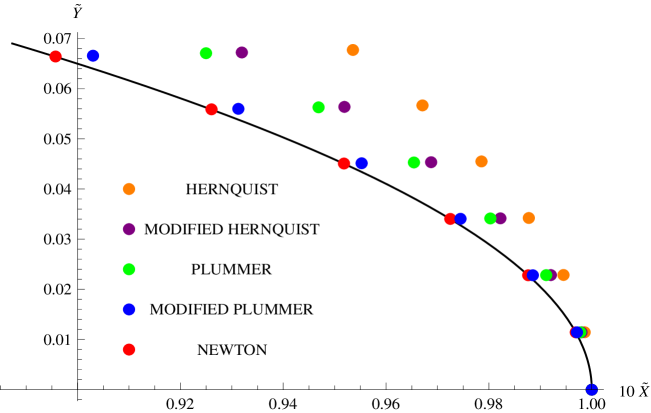
Figure 1: Trajectories for different potentials.

Orange points correspond to the modified equations of motion

$$\frac{d^{2}\tilde{X}}{d\tilde{t}^{2}}=-\frac{\tilde{X}}{(\tilde{R}+\tilde{\varepsilon})^{2}\tilde{R}},\quad\frac{d^{2}\tilde{Y}}{d\tilde{t}^{2}}=-\frac{\tilde{Y}}{(\tilde{R}+\tilde{\varepsilon})^{2}\tilde{R}}\,,$$ (3.5)

i.e. to the ”Newton – Hernquist” conversion

$$\frac{1}{\tilde{R}}\rightarrow\frac{1}{\tilde{R}+\tilde{\varepsilon}}$$ (3.6)

in the expression for the gravitational potential. The normalized softening length $\tilde{\varepsilon}$ everywhere equals $0.05$ (that is $\tilde{\varepsilon}$ amounts to $50\,\%$ of $\tilde{R}_{\mathrm{min}}$: $\tilde{\varepsilon}=\tilde{R}_{\mathrm{min}}/2$, meaning quite close approaching). Obviously, the orange points lie rather far from the red ones. Consequently, the error is significant.

Further, one obtains purple points modifying the Hernquist potential:

$$\frac{1}{\tilde{R}+\tilde{\varepsilon}}\rightarrow\frac{2}{\tilde{R}+\tilde{\varepsilon}}-\frac{1}{\tilde{R}+2\tilde{\varepsilon}}\,.$$ (3.7)

The idea underlying this modification is simple: at each iteration one can make calculations using both $\tilde{\varepsilon}$ and $2\tilde{\varepsilon}$ softenings and then interpolating results to the zero softening parameter. In other words, the expression in the right hand side of (3.7) is constructed purposely in such a way that for $\tilde{R}\gg\tilde{\varepsilon}$ its derivative with respect to $\tilde{R}$, being proportional to the gravitation force, behaves as $-1/\tilde{R}^{2}+6/\tilde{R}^{2}\cdot(\tilde{\varepsilon}/\tilde{R})^{2}$ up to the second order of smallness concerning the ratio $\tilde{\varepsilon}/\tilde{R}$. The term of the first order is missing, therefore, the actual superposition of two Hernquist potentials with different softenings reduces the simulation error in comparison with the previous case. Really, the purple points are noticeably closer to the red ones, then the orange points. However, precision is still low. Of course, one can increase a number of terms in the superposition and apply a higher order interpolation, but introduction of each additional term requires more computational time and, consequently, is not reasonable.

Green points correspond to the modified equations of motion

$$\frac{d^{2}\tilde{X}}{d\tilde{t}^{2}}=-\frac{\tilde{X}}{(\tilde{R}^{2}+\tilde{\varepsilon}^{2})^{3/2}},\quad\frac{d^{2}\tilde{Y}}{d\tilde{t}^{2}}=-\frac{\tilde{Y}}{(\tilde{R}^{2}+\tilde{\varepsilon}^{2})^{3/2}}\,,$$ (3.8)

i.e. to the ”Newton – Plummer” conversion

$$\frac{1}{\tilde{R}}\rightarrow\frac{1}{\sqrt{\tilde{R}^{2}+\tilde{\varepsilon}^{2}}}$$ (3.9)

in the expression for the gravitational potential. Precision is higher than in the previous case because the derivative of the expression in the right hand side of (3.9) with respect to $\tilde{R}$ for $\tilde{R}\gg\tilde{\varepsilon}$ behaves as $-1/\tilde{R}^{2}+1.5/\tilde{R}^{2}\cdot(\tilde{\varepsilon}/\tilde{R})^{2}$, so the deviation from the pure Newtonian behavior $-1/\tilde{R}^{2}$ is now four times smaller.

Finally, one gets blue points modifying the Plummer potential [18]:

$$\frac{1}{\sqrt{\tilde{R}^{2}+\tilde{\varepsilon}^{2}}}\rightarrow\frac{1}{(\tilde{R}^{4}+\tilde{\varepsilon}^{4})^{1/4}}\,.$$ (3.10)

Now for $\tilde{R}\gg\tilde{\varepsilon}$ the deviation from the pure Newtonian behavior represents a quantity of the forth order of smallness concerning the ratio $\tilde{\varepsilon}/\tilde{R}$. Consequently, precision is really high even despite the fact that the condition $\tilde{\varepsilon}=\tilde{R}_{\mathrm{min}}/2$ holds true as before.

4 Conclusion

In this paper a promising opportunity of increasing the accuracy of computer $N$-body simulations based on the PP method is addressed. Namely, the inevitable error arising from gravitational softening is reduced considerably by modifying the commonly used Plummer $\sim 1/\sqrt{R^{2}+\varepsilon^{2}}$ and Hernquist $\sim 1/(R+\varepsilon)$ potentials. In particular, the proposed $\sim 1/\left(R^{n}+\varepsilon^{n}\right)^{1/n}$ potential with $n>2$ gives better approximation since for $R>\varepsilon$ the corresponding gravitation force differs from the standard Newtonian one in a small quantity $\sim(\varepsilon/R)^{n}$. This is demonstrated explicitly for $n=4$ with the help of the concrete illustrative example of one particle moving along the hyperbolic trajectory in the softened gravitational field of another one. The force resolution $\varepsilon$ is taken amounting to half the minimum separation distance, but despite this fact the suggested alternative softening is characterized by much higher precision being much closer to the pure Newtonian picture than the standard ones.

Apparently, while improving numerical integration in the region $R>\varepsilon$ (where owing to this important inequality the expansion into series with respect to the ratio $\varepsilon/R<1$ is allowed), the developed scheme still misrepresents the picture for $R\leqslant\varepsilon$ (where the above-mentioned expansion is forbidden). However, if such close approachings happen seldom, this misrepresentation is not significant for the whole $N$-body system behavior description. Thus, this scheme can really play an important role in astrophysical/cosmological modeling and solving the above-mentioned Problem 5. In other words, the proposed modifications reducing simulation errors caused by softening can help to bring the phase trajectory of the $N$-body system in a corresponding computer code much closer to that of the real physical one.

References

- [1] V.G. Gurzadyan, 10 key problems in stellar dynamics: in retrospect. In: ”Ergodic Concepts in Stellar Dynamics”, Eds. V.G. Gurzadyan, D. Pfenniger, Lecture Notes in Physics 430, p. 281-284 (Problems), p. 285-291 (Comments on key problems), Springer, 1994; (arXiv:astro-ph/1407.0398).
- [2] S.J. Aarseth, Gravitational N-body simulations: tools and algorithms, Cambridge University Press, 2003.
- [3] J. Makino, T. Fukushige, M. Koga and K. Namura, GRAPE-6: massively-parallel special-purpose computer for astrophysical particle simulations, PASJ 55 (2003) 1163.
- [4] M. Eingorn and A. Zhuk, Hubble flows and gravitational potentials in observable Universe, JCAP 09 (2012) 026; (arXiv:astro-ph/1205.2384).
- [5] M. Eingorn, A. Kudinova and A. Zhuk, Dynamics of astrophysical objects against the cosmological background, JCAP 04 (2013) 010; (arXiv:astro-ph/1211.4045).
- [6] M. Eingorn and A. Zhuk, Remarks on mechanical approach to observable Universe, JCAP 05 (2014) 024; (arXiv:astro-ph/1309.4924).
- [7] P.J.E. Peebles, The large-scale structure of the Universe, Princeton University Press, Princeton (1980).
- [8] V. Springel, The cosmological simulation code GADGET-2, MNRAS 364 (2005) 1105; (arXiv:astro-ph/0505010).
- [9] L.D. Landau and E.M. Lifshitz, The Classical Theory of Fields, Fourth Edition: Volume 2 (Course of Theoretical Physics Series), Oxford Pergamon Press, Oxford (2000).
- [10] M. Eingorn, M. Brilenkov and B. Vlahovic, Zero average values of cosmological perturbations as an indispensable condition for the theory and simulations (2014); (arXiv:astro-ph/1407.3244).
- [11] H.C. Plummer, On the problem of distribution in globular star clusters, MNRAS 71 (1911) 460.
- [12] K. Dolag, S. Borgani, S. Schindler, A. Diaferio and A.M. Bykov, Simulation techniques for cosmological simulations, Space Science Reviews 134 (2008) 229; (arXiv:astro-ph/0801.1023).
- [13] F. Iannuzzi and K. Dolag, Adaptive gravitational softening in GADGET, MNRAS 417 (2011) 2846; (arXiv:astro-ph/1107.2942).
- [14] J.E. Barnes, Gravitational softening as a smoothing operation, MNRAS 425 (2012) 1104; (arXiv:astro-ph/1205.2729).
- [15] B. Röttgers, T. Naab and L. Oser, Stellar orbits in cosmological galaxy simulations: the connection to formation history and line-of-sight kinematics; (arXiv:astro-ph/1406.6696).
- [16] L. Hernquist, An analytical model for spherical galaxies and bulges, Astrophysical Journal 356 (1990) 359.
- [17] L.D. Landau and E.M. Lifshitz, Mechanics, Third Edition: Volume 1 (Course of Theoretical Physics Series), Oxford Pergamon Press, Oxford (2000).
- [18] K.S. Oh, D.N.C. Lin and S.J. Aarseth, On the tidal disruption of dwarf spheroidal galaxies around the galaxy, Astrophysical Journal 442 (1995) 142.