High-order adaptive time stepping for vesicle suspensions with viscosity contrast

Abstract

We construct a high-order adaptive time stepping scheme for vesicle suspensions with viscosity contrast. The high-order accuracy is achieved using a spectral deferred correction (SDC) method, and adaptivity is achieved by estimating the local truncation error with the numerical error of physically constant values. Numerical examples demonstrate that our method can handle suspensions with vesicles that are tumbling, tank-treading, or both. Moreover, we demonstrate that a user-prescribed tolerance can be automatically achieved for simulations with long time horizons.

1 Introduction

Vesicles are deformable capsules filled with an incompressible viscous fluid. Their mechanical properties are characterized by bending resistance and tension that enforces local inextensibility of their membrane. We are interested in the fluid mechanics of vesicles suspensions where the bulk fluid is a Newtonian incompressible fluid. The hydrodynamics of vesicles play an important role in many biological phenomena [1, 2]. For example, they are used experimentally to understand properties of biomembranes [3] and red blood cells [4, 5, 6, 7, 8]. Here we extend our work on high-order adaptive time integrators [9] to vesicle suspensions with viscosity contrast; that is, the viscosity in the interior of each vesicle is constant, but can differ from the constant viscosity of the exterior fluid. This extension is important for applications such as, for example, simulating microfluidic devices that sort red blood cells of different viscosity contrasts. By using an adaptive high-order time integrator, we can efficiently simulate suspensions to a user-specified tolerance without requiring a trial and error procedure. Moreover, by using a high-order method, fewer time steps are required when the desired tolerance is small. This paper is a key step towards a black-box solver for vesicle suspensions with long time horizons and that exhibit dynamics of varying complexity.

The most significant limitation of this work is that it is implemented only in two dimensions. Fortunately, the time integrator and adaptivity strategy we introduce is independent of the dimension and we plan to extend this work to three dimensions in the future. While we now allow for variable time step sizes, we do not address multirate time integrators. That is, at each time step, the same time step size is applied to all the vesicles. In addition to time adaptivity, spatial adaptivity also needs to be addressed in the future. Since vesicles may develop and smooth regions of high curvature, allowing for only one spatial grid is inefficient. In this paper, the spatial domain is fixed for the entire simulation but, in the numerical examples, when performing a convergence study in time, we choose a spatial discretization that is sufficiently large that the temporal error dominates.

Vesicle suspensions, in two and three dimensions, have been well-studied and we refrain from doing a thorough literature review of their physics. Instead, we focus on work related to our time integrator. The spectral deferred correction (SDC) method was first introduced but Dutt, Greengard, and Rokhlin [10]. In its original form, it was a stable method to construct high-order solutions of initial value problems. It was extended to implicit-explicit (IMEX) methods by Minion [11], where the splitting between stiff and non-stiff terms is additive. SDC has also been used as a parallel-in-time time stepper [12], but this work only considers initial value problems which are much cheaper to solve than the integro-differential equations we solve. SDC has been used for an integro-differential equation [13] that simulates a diffusion process with moving interfaces, but their governing equations are less stiff and the interface equations are simpler than ours. To the best of our knowledge, our work [9] is the first to apply SDC to an operator-based IMEX splitting of the equations governing vesicle suspensions. It is this work that we now extend to vesicles with viscosity contrast.

The remainder of the paper is organized as follows. In Section 2 we present equations that govern vesicle dynamics, reformulate them in terms of integral equations, and introduce SDC. In Section 3, the numerical schemes for the governing equations are presented and we discuss the adaptive time stepping strategy. In Section 4, we present two numerical results, and we make concluding remarks in Section 5.

2 Formulation

Neglecting inertial forces, the dynamics of a vesicle is fully characterized by the position of the interface ${\mathbf{x}}(s,t)\in\gamma$, where $s$ is the arclength, $t$ is time, and $\gamma$ is the membrane of the vesicle. The position is determined by solving a moving interface problem that models the mechanical interactions between the viscous incompressible fluid in the exterior and interior of the vesicle and the vesicle membrane, all the while, requiring that the membrane maintains its length (inextensibility condition). In addition to the position ${\mathbf{x}}(s,t)$, the other main variables are the fluid velocity ${\mathbf{u}}$, the fluid stress $T$, the pressure $p$, the membrane tension $\sigma$, and the stress jump across $\gamma$, ${\mathbf{f}}({\mathbf{x}})=\llbracket T\rrbracket\mathbf{n}$, where $\mathbf{n}$ is the unit outward normal. The stress jump is equal to the sum of a force due to the vesicle membrane bending modulus $\kappa_{b}$ and a force due to the tension $\sigma$.

Given these definitions, the equations for an unbounded suspension of vesicles are

$$\begin{aligned} \mu{\triangledown}\cdot({\triangledown}{\mathbf{u}}+{\triangledown}{\mathbf{u}}^{T})={\triangledown}p({\mathbf{x}}),&\hskip 20.0pt{\mathbf{x}}\in{\mathbb{R}}^{2}\backslash\gamma,\hskip 14.45377pt&&\mbox{conservation of momentum},\\ {\triangledown}\cdot{\mathbf{u}}({\mathbf{x}})=0,&\hskip 20.0pt{\mathbf{x}}\in{\mathbb{R}}^{2}\backslash\gamma,\hskip 14.45377pt&&\mbox{conservation of mass},\\ {\mathbf{u}}({\mathbf{x}},t)={\mathbf{v}}_{\infty}({\mathbf{x}}),&\hskip 20.0pt|{\mathbf{x}}|\rightarrow\infty,\hskip 14.45377pt&&\mbox{far-field velocity},\\ \dot{{\mathbf{x}}}(t)={\mathbf{u}}({\mathbf{x}},t),&\hskip 20.0pt{\mathbf{x}}\in\gamma,\hskip 14.45377pt&&\mbox{velocity continuity},\\ \llbracket T\rrbracket\mathbf{n}=-\kappa_{b}{\mathbf{x}}_{ssss}+(\sigma({\mathbf{x}}){\mathbf{x}}_{s})_{s},&\hskip 20.0pt{\mathbf{x}}\in\gamma,\hskip 14.45377pt&&\mbox{nonzero stress jump},\\ {\mathbf{x}}_{s}\cdot{\mathbf{u}}_{s}=0,&\hskip 20.0pt{\mathbf{x}}\in\gamma,\hskip 14.45377pt&&\mbox{membrane inextensibility}.\\ \end{aligned}$$ (1)

While the viscosity is taken to be constant inside each vesicle, these values can differ from the viscosity of the exterior fluid. In particular, we define the viscosity contrast $\nu_{p}=\mu_{p}/\mu_{0}$.

Since the viscosity is piecewise constant with a discontinuity along the interface, we use an integral equation formulation using the Stokes free-space Green’s function [14]. We introduce the following integral and differential operators that we use to formulate (1) in terms of unknowns that are defined only on the vesicle boundary $\gamma$:

• Single- and double-layer potentials:

  $$\SS(\gamma_{j},\gamma_{k}){\mathbf{f}} :=\frac{1}{4\pi\mu_{0}}\int_{\gamma_{k}}\left(-\boldsymbol{I}\log\rho+\frac{{\mathbf{r}}\otimes{\mathbf{r}}}{\rho^{2}}\right){\mathbf{f}}\,ds_{{\mathbf{y}}}, {\mathbf{x}}\in\gamma_{j},$$

  $${\mathcal{D}}(\gamma_{j},\gamma_{k}){\mathbf{u}} :=\frac{1-\nu_{k}}{\pi}\int_{\gamma_{k}}\frac{{\mathbf{r}}\cdot{\mathbf{n}}}{\rho^{2}}\frac{{\mathbf{r}}\otimes{\mathbf{r}}}{\rho^{2}}{\mathbf{u}}\,ds_{{\mathbf{y}}}, {\mathbf{x}}\in\gamma_{j},$$

  where ${\mathbf{r}}={\mathbf{x}}-{\mathbf{y}}$, $\rho=\|{\mathbf{r}}\|$, and ${\mathbf{n}}$ is the outward unit normal of $\gamma_{k}$.

• Bending, tension, and surface divergence:

  $${\mathcal{B}}(\gamma_{k}){\mathbf{f}}:=\kappa_{b}\frac{d^{4}}{ds^{4}}{\mathbf{f}},\quad{\mathcal{T}}(\gamma_{k})\sigma:=(\sigma{\mathbf{x}}_{s})_{s},\quad{\mathrm{Div}}(\gamma_{k}){\mathbf{f}}:=\frac{d{\mathbf{x}}}{ds}\cdot\frac{d{\mathbf{f}}}{ds},$$

  where each arclength derivative is taken with respect to ${\mathbf{x}}_{k}$, and $\kappa_{b}$ is the bending modulus.

Note that all these operators are linear once $\gamma_{j}$ and $\gamma_{k}$ are fixed.

2.1 Integral equation formulation

Let $\omega_{j}$, $j=1,\dots,M$, be the interior of vesicle $j$. An integral equation representation of the fluid velocity is [15]

$$\alpha{\mathbf{u}}({\mathbf{x}})={\mathbf{v}}_{\infty}({\mathbf{x}})+\sum_{k=1}^{M}\SS({\mathbf{x}},{\mathbf{x}}_{k})\left(-{\mathcal{B}}({\mathbf{x}}_{k}){\mathbf{x}}_{k}+{\mathcal{T}}({\mathbf{x}}_{k})\sigma_{k}\right)+\sum_{k=1}^{M}{\mathcal{D}}({\mathbf{x}},{\mathbf{x}}_{k}){\mathbf{u}}({\mathbf{x}}_{k}),\quad{\mathbf{x}}\in{\mathbb{R}}^{2},$$

where

$$\alpha=\left\{\begin{array}[]{ll}\nu_{j}&\hskip 14.45377pt{\mathbf{x}}\in\omega_{j},\\ \frac{1+\nu_{j}}{2}&\hskip 14.45377pt{\mathbf{x}}\in\gamma_{j},\\ 1&\hskip 14.45377pt{\mathbf{x}}\in{\mathbb{R}}^{2}\backslash\overline{\omega_{j}}.\end{array}\right.$$

Applying the no-slip boundary condition on the boundary of the vesicle, we have

$$\alpha_{j}\frac{d{\mathbf{x}}_{j}}{dt}={\mathbf{v}}_{\infty}({\mathbf{x}}_{j})+\sum_{k=1}^{M}\SS({\mathbf{x}}_{j},{\mathbf{x}}_{k})\left(-{\mathcal{B}}({\mathbf{x}}_{k}){\mathbf{x}}_{k}+{\mathcal{T}}({\mathbf{x}}_{k})\sigma_{k}\right)+\sum_{k=1}^{M}{\mathcal{D}}({\mathbf{x}}_{j},{\mathbf{x}}_{k})\frac{d{\mathbf{x}}_{k}}{dt},\quad\alpha_{j}=\frac{1+\nu_{j}}{2}.$$

The tension $\sigma$ acts as a Lagrange multiplier to impose the inextensibility condition ${\mathrm{Div}}({\mathbf{x}}_{j})\frac{d{\mathbf{x}}_{j}}{dt}=0$. In order to ease the presentation, we abuse notation by dropping the subscripts and summations, and we write

$$\alpha\frac{d{\mathbf{x}}}{dt}={\mathbf{v}}_{\infty}({\mathbf{x}})+\SS({\mathbf{x}})\left(-{\mathcal{B}}({\mathbf{x}}){\mathbf{x}}+{\mathcal{T}}({\mathbf{x}})\sigma\right)+{\mathcal{D}}({\mathbf{x}})\frac{d{\mathbf{x}}}{dt},\quad\alpha=\frac{1+\nu}{2},$$ (2)

with the inextensibility condition ${\mathrm{Div}}({\mathbf{x}})\frac{d{\mathbf{x}}}{dt}=0$.

In the SDC framework, it is convenient to reformulate (2) as the Picard integral

$${\mathbf{x}}(t)={\mathbf{x}}_{0}+\int_{0}^{t}(\alpha I-{\mathcal{D}}({\mathbf{x}}))^{-1}({\mathbf{v}}_{\infty}({\mathbf{x}})-\SS({\mathbf{x}})({\mathcal{B}}({\mathbf{x}}){\mathbf{x}}+{\mathcal{T}}({\mathbf{x}})\sigma))d\tau.$$ (3)

A similar Picard integral can be derived for confined flows by replacing ${\mathbf{v}}_{\infty}$ with a double-layer potential with an unknown density function defined on the solid walls [9]. Then, a no-slip boundary condition on the solid walls results in a second-kind integral equation that must also be satisfied. In this work, for simplicity, we only present results for unbounded flows.

2.2 Spectral Deferred Correction

Spectral deferred correction (SDC) is an iterative method for solving Picard integral equations such as (3). It was first introduced as a stable deferred correction method for solving initial value problems [10]. Our SDC formulation is most closely related to the work of Minion [11] who was the first to investigate the coupling of SDC with IMEX time integrators. We first compute a provisional solution ${\tilde{{\mathbf{x}}}}$ and ${\tilde{\sigma}}$ using some time integrator, and then form the residual of (3)

$${\mathbf{r}}(t):={\mathbf{x}}_{0}-{\tilde{{\mathbf{x}}}}(t)+\int_{0}^{t}{\tilde{{\mathbf{v}}}}(\tau)d\tau,$$ (4)

where the provisional velocity is ${\tilde{{\mathbf{v}}}}=(\alpha I-{\mathcal{D}}({\tilde{{\mathbf{x}}}}))^{-1}({\mathbf{v}}_{\infty}({\tilde{{\mathbf{x}}}})-\SS({\tilde{{\mathbf{x}}}}){\mathcal{B}}({\tilde{{\mathbf{x}}}}){\tilde{{\mathbf{x}}}}+\SS({\tilde{{\mathbf{x}}}}){\mathcal{T}}({\tilde{{\mathbf{x}}}}){\tilde{\sigma}})$. We now define the errors in position, $\mathbf{e}_{{\mathbf{x}}}:={\mathbf{x}}-{\tilde{{\mathbf{x}}}}$, and tension, $e_{\sigma}:=\sigma-{\tilde{\sigma}}$. By substituting $\mathbf{e}_{{\mathbf{x}}}$ and $e_{\sigma}$ into (3), we have

$$\mathbf{e}_{{\mathbf{x}}}(t)={\mathbf{x}}_{0}-{\tilde{{\mathbf{x}}}}(t)+\int_{0}^{t}(\alpha I-{\mathcal{D}}({\tilde{{\mathbf{x}}}}+\mathbf{e}_{{\mathbf{x}}}))^{-1}({\mathbf{v}}_{\infty}({\tilde{{\mathbf{x}}}}+\mathbf{e}_{{\mathbf{x}}})-\SS({\tilde{{\mathbf{x}}}}+\mathbf{e}_{{\mathbf{x}}}){\mathcal{B}}({\tilde{{\mathbf{x}}}}+\mathbf{e}_{{\mathbf{x}}})({\tilde{{\mathbf{x}}}}+\mathbf{e}_{{\mathbf{x}}})+\SS({\tilde{{\mathbf{x}}}}+\mathbf{e}_{{\mathbf{x}}}){\mathcal{T}}({\tilde{{\mathbf{x}}}}+\mathbf{e}_{{\mathbf{x}}})({\tilde{\sigma}}+e_{\sigma}))d\tau.$$

Following the usual SDC framework, we introduce the residual into the error equation

$$\begin{split}\mathbf{e}_{{\mathbf{x}}}(t)&={\mathbf{r}}(t)+\int_{0}^{t}\left\{(\alpha I-{\mathcal{D}}({\tilde{{\mathbf{x}}}}+\mathbf{e}_{{\mathbf{x}}}))^{-1}{\mathbf{v}}_{\infty}({\tilde{{\mathbf{x}}}}+\mathbf{e}_{{\mathbf{x}}})-(\alpha I-{\mathcal{D}}({\tilde{{\mathbf{x}}}}))^{-1}{\mathbf{v}}_{\infty}({\tilde{{\mathbf{x}}}})\right\}d\tau\\ &+\int_{0}^{t}\left\{-(\alpha I-{\mathcal{D}}({\tilde{{\mathbf{x}}}}+\mathbf{e}_{{\mathbf{x}}}))^{-1}\SS({\tilde{{\mathbf{x}}}}+\mathbf{e}_{{\mathbf{x}}}){\mathcal{B}}({\tilde{{\mathbf{x}}}}+\mathbf{e}_{{\mathbf{x}}})+(\alpha I-{\mathcal{D}}({\tilde{{\mathbf{x}}}}))^{-1}\SS({\tilde{{\mathbf{x}}}}){\mathcal{B}}({\tilde{{\mathbf{x}}}})\right\}{\tilde{{\mathbf{x}}}}d\tau\\ &+\int_{0}^{t}\left\{(\alpha I-{\mathcal{D}}({\tilde{{\mathbf{x}}}}+\mathbf{e}_{{\mathbf{x}}}))^{-1}\SS({\tilde{{\mathbf{x}}}}+\mathbf{e}_{{\mathbf{x}}}){\mathcal{T}}({\tilde{{\mathbf{x}}}}+\mathbf{e}_{{\mathbf{x}}})-(\alpha I-{\mathcal{D}}({\tilde{{\mathbf{x}}}}))^{-1}\SS({\tilde{{\mathbf{x}}}}){\mathcal{T}}({\tilde{{\mathbf{x}}}})\right\}{\tilde{\sigma}}d\tau\\ &+\int_{0}^{t}(\alpha I-{\mathcal{D}}({\tilde{{\mathbf{x}}}}+\mathbf{e}_{{\mathbf{x}}}))^{-1}\left\{-\SS({\tilde{{\mathbf{x}}}}+\mathbf{e}_{{\mathbf{x}}}){\mathcal{B}}({\tilde{{\mathbf{x}}}}+\mathbf{e}_{{\mathbf{x}}})\mathbf{e}_{{\mathbf{x}}}+\SS({\tilde{{\mathbf{x}}}}+\mathbf{e}_{{\mathbf{x}}}){\mathcal{T}}({\tilde{{\mathbf{x}}}}+\mathbf{e}_{{\mathbf{x}}})e_{\sigma}\right\}d\tau.\end{split}$$ (5)

Finally, the inextensibility constraint is ${\mathrm{Div}}({\tilde{{\mathbf{x}}}}+\mathbf{e}_{{\mathbf{x}}})\frac{d({\tilde{{\mathbf{x}}}}+\mathbf{e}_{{\mathbf{x}}})}{dt}=0$.

3 Numerical Scheme

Several challenges arise when forming numerical solutions of (3) (and (5)). For instance, the bending operator ${\mathcal{B}}$ introduces stiffness which is resolved by using a semi-implicit discretization of (3). Another challenge is to accurately approximate the layer potentials $\SS$ and ${\mathcal{D}}$ for vesicles that are arbitrarily close to one another which is resolved with specialized quadrature that efficiently handles near-singular integrals. Additional complications and more details are discussed in previous work [16, 17]. Here we focus on the numerical aspects associated with solving (3), (4), (5), and with computing optimal time step sizes.

SDC is an iterative method that computes successively more accurate solutions of (3). The SDC iteration is

1. Form a provisional solution ${\tilde{{\mathbf{x}}}}$ and ${\tilde{\sigma}}$ of (3)

2. Form the residual (4) of the provisional solution.

3. Compute an approximate solution of the error equation (5).

4. Define the provisional solution as ${\tilde{{\mathbf{x}}}}+\mathbf{e}_{{\mathbf{x}}}$ and ${\tilde{\sigma}}{}+e_{\sigma}$.

5. If desired, return to step 2.

We have numerically shown [9] that if (3) and (5) are solved with first-order methods, then after $n_{{\mathrm{sdc}}}$ SDC iterations, the order of accuracy of the solution is $n_{{\mathrm{sdc}}}+1$, as long as this order does not exceed the order of accuracy of the quadrature formula for ${\mathbf{r}}$.

3.1 Discretization of the Picard integral

A first-order approximation of (3) is formed using the semi-implicit time integrator

$$\alpha\frac{{\mathbf{x}}^{N+1}-{\mathbf{x}}^{N}}{\Delta t}={\mathbf{v}}_{\infty}^{N}+\SS^{N}\left(-{\mathcal{B}}^{N}{\mathbf{x}}^{N+1}+{\mathcal{T}}^{N}\sigma^{N+1}\right)+{\mathcal{D}}^{N}\left(\frac{{\mathbf{x}}^{N+1}-{\mathbf{x}}^{N}}{\Delta t}\right).$$ (6)

The time integrator (6) treats both intra- and inter-vesicle interactions semi-implicitly, with the latter resolving stiffness introduced by vesicles that are close to one another. We solve (6) with the generalized minimal residual method (GMRES) with an exact block-diagonal preconditioner. This method has been thoroughly tested for stability, first-order convergence, and GMRES iteration mesh-independence on a variety of vesicle suspensions [17].

To compute the residual (4), we approximate (3) at $p$ substeps of $[0,\Delta t]$, and then use an appropriate quadrature formula to compute ${\mathbf{r}}$. To achieve high-order accuracy, avoid extrapolation, and minimize the Runge phenomenon, we use Gauss-Lobatto points, whose quadrature error is $\mathcal{O}(\Delta t^{2p-3})$. Once a provisional first-order solution and the residual are computed, the error equation (5) is numerically solved for $\mathbf{e}_{{\mathbf{x}}}$ and $e_{\sigma}$. We discretize (5) by dropping all the terms except the first and the last

$$\alpha\frac{\mathbf{e}_{{\mathbf{x}}}^{N+1}-\mathbf{e}_{{\mathbf{x}}}^{N}}{\Delta t}=\left(\alpha I-{\mathcal{D}}^{N+1}\right)\left(\frac{{\mathbf{r}}^{N+1}-{\mathbf{r}}^{N}}{\Delta t}\right)+\SS^{N+1}\left(-{\mathcal{B}}^{N+1}\mathbf{e}_{{\mathbf{x}}}^{N+1}+{\mathcal{T}}^{N+1}e_{\sigma}^{N+1}\right)+{\mathcal{D}}^{N+1}\left(\frac{\mathbf{e}_{{\mathbf{x}}}^{N+1}-\mathbf{e}_{{\mathbf{x}}}^{N}}{\Delta t}\right),$$ (7)

and we have observed numerically [9] that each solution of (7) results in an additional order of convergence. In (7), the operators are discretized at ${\tilde{{\mathbf{x}}}}^{N+1}$ which is computed when the provisional solution is formed. Now, equations (6) and (7) require inverting the same linear system; the only differences are the right hand side and the state at which the operators are discretized. We also note that if this iteration converges, that is, $\mathbf{e}_{{\mathbf{x}}}\rightarrow 0$ and $e_{\sigma}\rightarrow 0$, then ${\mathbf{r}}^{N+1}={\mathbf{r}}^{N}$, implying that the Picard integral (3) has been solved up to quadrature error.

3.2 Discretization of the inextensibility condition

Based on our first-order discretization (6), the inextensibility condition ${\mathrm{Div}}({\mathbf{x}})(d{\mathbf{x}}/dt)=0$ for the provisional solution is equivalent to ${\mathrm{Div}}({\mathbf{x}}^{N}){\mathbf{x}}^{N+1}=1$. Once the provisional solution ${\tilde{{\mathbf{x}}}}$ and ${\tilde{\sigma}}$ have been computed, the inextensibility condition is ${\mathrm{Div}}({\tilde{{\mathbf{x}}}}+\mathbf{e}_{{\mathbf{x}}})\frac{d({\tilde{{\mathbf{x}}}}+\mathbf{e}_{{\mathbf{x}}})}{dt}=0$, which, using the first-order discretization (7) is equivalent to

$${\mathrm{Div}}^{N+1}(\mathbf{e}_{{\mathbf{x}}}^{N+1})={\mathrm{Div}}^{N+1}(\mathbf{e}_{{\mathbf{x}}}^{N})+{\mathrm{Div}}^{N+1}({\mathbf{r}}^{N+1}-{\mathbf{r}}^{N}+\Delta t_{N}{\tilde{{\mathbf{v}}}}^{N+1}),$$

where $\Delta t_{N}$ is the size of the substep. Unfortunately, we have experimentally found that this discretization requires a very small time step before SDC converges. As an alternative, we formulate the inextensibility constraint as

$$({\tilde{{\mathbf{x}}}}^{N+1}+\mathbf{e}_{{\mathbf{x}}}^{N+1})_{s_{0}}\cdot({\tilde{{\mathbf{x}}}}^{N+1}+\mathbf{e}_{{\mathbf{x}}}^{N+1})_{s_{0}}=1,$$

where $s_{0}$ is the arclength component of the vesicle at the initial Gauss-Lobatto point. Assuming that the error $\mathbf{e}_{{\mathbf{x}}}$ is much smaller than ${\tilde{{\mathbf{x}}}}$, we can neglect the quadratic term and enforce inextensibility by requiring

$${\tilde{{\mathbf{x}}}}^{N+1}_{s_{0}}\cdot(\mathbf{e}_{{\mathbf{x}}}^{N+1})_{s_{0}}=\frac{1}{2}(1-{\tilde{{\mathbf{x}}}}_{s_{0}}^{N+1}\cdot{\tilde{{\mathbf{x}}}}_{s_{0}}^{N+1}).$$ (8)

Because the arclength term is discretized at $s_{0}$, the inextensibility condition for the error (8) differs slightly from the inextensibility condition for the provisional solution. However, the resulting system converges for much larger values of $\Delta t$ and, if $\mathbf{e}_{{\mathbf{x}}}\rightarrow 0$, then the inextensibility condition ${\tilde{{\mathbf{x}}}}^{N+1}_{s_{0}}\cdot{\tilde{{\mathbf{x}}}}^{N+1}_{s_{0}}=1$ is exactly satisfied.

3.3 Time step size selection

During the course of a vesicle simulation, it is advantageous to adjust the time step size based on the complexity of the dynamics. For instance, when a vesicle has regions of high curvature or two vesicles are close to one another, a smaller time step should be taken. The main advantages of an adaptive time step size are: the simulation is sped up since the largest allowable time step size is taken; and, no trial and error procedure is necessary to find a time step size that achieves a desired tolerance.

We adopt the common strategy of controlling an estimate of the local truncation error [18]. Because of the inextensibility and incompressibility conditions, vesicle suspensions have a natural estimate of the local truncation error: the errors in area and length. The advantage of this estimate is that multiple numerical solutions do not need to be formed to estimate the local truncation error. For a single vesicle (multiple vesicles are handled by taking the maximum over all the errors in area and length), let the area and length at time $t$ be $A(t)$ and $L(t)$, and suppose that the desired tolerance for the global error is $\epsilon$ at the normalized time horizon $T=1$. We compute the solution at time $t+\Delta t$ using a time stepping scheme and then compute the new area $A(t+\Delta t)$ and length $L(t+\Delta t)$. The solution is accepted only if

$$|A(t+\Delta t)-A(t)|\leq\frac{A(t)\Delta t}{1-t}\left(\epsilon-\frac{|A(t)-A(0)|}{A(t)}\right),$$ (9)

and a similar condition for the length. Instead of the usual condition $|A(t+\Delta t)-A(t)|\leq A(t)\Delta t\epsilon$, we are adjusting the amount of local truncation error that can be committed in $[t,t+\Delta t]$ based on the error committed in $[0,t]$. Using this strategy, our scheme can commit larger local truncation errors than $\epsilon\Delta t$ if the error committed in $[0,t]$ is less than $\epsilon t$.

Regardless of the acceptance or rejection of the solution at time $t+\Delta t$, a new time step size must be chosen. Based on an asymptotic argument [9], to make the bound in (9) tight, the optimal time step size is

$$\Delta t_{{\mathrm{opt}}}=\left\{\frac{A(t)}{|A(t+\Delta t)-A(t)|}\frac{\Delta t}{1-t}\left(\epsilon-\frac{|A(t)-A(0)|}{A(t)}\right)\right\}^{1/k}\Delta t,$$

where $k$ is the order of the time integrator. A similar optimal time step size is computed based on the length and the smaller of these values is used to compute the next time step size. Since the choice of $\Delta t_{{\mathrm{opt}}}$ assumes that the error is in the asymptotic regime, we impose several safety factors on the new time step size $\Delta t_{{\mathrm{new}}}$. First, we require $\Delta t_{{\mathrm{new}}}/\Delta t\in[\beta_{{\mathrm{down}}},\beta_{{\mathrm{up}}}]$, where $\beta_{{\mathrm{down}}}=0.6$ and $\beta_{{\mathrm{up}}}=1.5$. That is, the time step size is not allowed to change too quickly. Next, we multiply the new time step size by a safety factor $\beta_{{\mathrm{scale}}}=\sqrt{0.9}$ to increase the likelihood of the next time step size being accepted. These three parameters are chosen from experience and can be changed if required by a certain application. As a final restriction, we never increase the time step size if the previous time step size is rejected [18]. In summary, if the previous time step is accepted, the new time step size is

$$\Delta t_{{\mathrm{new}}}=\beta_{{\mathrm{scale}}}^{1/k}\min(\beta_{{\mathrm{up}}}\Delta t,\max(\Delta t_{{\mathrm{opt}}},\beta_{{\mathrm{down}}}\Delta t)),$$

and if the previous time step is rejected, the new time step size is

$$\Delta t_{{\mathrm{new}}}=\beta_{{\mathrm{scale}}}^{1/k}\min(\Delta t,\max(\Delta t_{{\mathrm{opt}}},\beta_{{\mathrm{down}}}\Delta t)).$$

4 Numerical Examples

We consider vesicles with reduced area 0.66, initially parameterized as ${\mathbf{x}}(\theta,0)=(\cos\theta,3\sin\theta)$, in the shear flow ${\mathbf{v}}_{\infty}=(y,0)$. We report the number of uniform time steps, $m$, the error in area, $e_{A}$, and the error in length, $e_{L}$. To evaluate the cost of the algorithm, we report the number of matrix-vector-multiplications, (“matvecs” for short), required to iteratively solve (6) and (7) and to compute the provisional velocity ${\tilde{{\mathbf{v}}}}$, and the CPU time required by Matlab on a six-core 2.67GHz Intel Xeon processor with 24GB of memory.

We first verify that our time integrator with one SDC correction provides second-order convergence. Then, we use this time integrator with an adaptive time step size for two different problems. We use $p=5$ Gauss-Lobatto substeps which achieves $7^{th}$-order accuracy when computing the residual ${\mathbf{r}}(t)$. We set the block-diagonal preconditioned GMRES tolerance to 1E-10 which, based on previous work [17, 9], is the smallest allowable tolerance due to the ill-conditioning of the governing equations.

4.1 Tank-treading and tumbling

We consider a single vesicle with two different viscosity contrasts, and discretized with $N=96$ points, which is sufficiently refined to guarantee that the temporal error dominates. We use a fixed time step size to verify that one SDC correction results in second-order convergence. Table 1 corresponds to a tank-treading vesicle ($\nu=4$) while Table 2 corresponds to a tumbling vesicle ($\nu=15$). With the prescribed time horizon, the tumbling vesicle makes approximately 2.5 rotations. In both regimes, we achieve in excess of second-order convergence but, in general, we only expect second-order convergence.

Table 1: The number of uniform time steps, errors in area and length, the number of matvecs, and the CPU time for a single vesicle in the tank-treading regime ($\nu=4$). We see that second-order (in fact, it is closer to third-order) convergence is achieved.

$m$	$e_{A}$	$e_{L}$	matvecs	CPU
75	1.39E-2	1.43E-2	9.45E3	8.16E1
150	1.42E-3	1.68E-3	1.60E4	1.53E2
300	1.14E-4	2.03E-4	2.81E4	2.88E2
600	8.33E-7	2.46E-5	5.16E4	5.68E2
1200	3.80E-6	2.99E-6	9.56E4	1.08E3

Table 2: The number of uniform time steps, errors in area and length, the number of matvecs, and the CPU time for a single vesicle in the tumbling regime ($\nu=15$). Again, second-order (in fact, it is closer to 2.5-order) convergence is achieved. Also, we see that GMRES requires fewer iterations to solve suspensions with larger viscosity contrasts, but larger global errors are incurred.

$m$	$e_{A}$	$e_{L}$	matvecs	CPU
75	1.25E-1	3.80E-2	8.40E3	7.94E1
150	2.07E-2	5.22E-3	1.45E4	1.55E2
300	3.27E-3	6.28E-4	2.57E4	2.83E2
600	5.51E-4	7.88E-5	4.68E4	5.38E2
1200	1.04E-4	9.89E-6	8.73E4	1.09E3

We now test our adaptive time stepper with viscosity contrast $\nu=4$ (Table 3), $\nu=10$ (Table 4), and $\nu=15$ (Table 5). In all of the examples, without any a priori knowledge of the time step size, the desired tolerance is achieved. Unsurprisingly, larger time steps can be taken when the vesicle is tank-treading ($\nu=4$) as opposed to tumbling ($\nu=10$ and $\nu=15$). In all three simulations, as the tolerance decreases, the number of required time steps grows unacceptably large. This can be resolved by taking two SDC corrections (bottom rows of Tables 3–4) at the expense of solving (5) twice instead of once which, in theory, results in a third-order time integrator. This additional solve is justified since the reduction in CPU time is 41% for $\nu=4$, 60% for $\nu=10$, and 63% for $\nu=15$. Therefore, we conclude that as more tolerance is requested, the additional cost of using additional SDC iterations is justified. In order to continue our development of a black-box solver for vesicle suspensions, a systematic method for choosing an appropriate number of SDC iterations based on the requested tolerance is under investigation.

Table 3: Adaptive time stepping with $\nu=4$. The adaptive time step size does a good job of achieving the desired tolerance with only a few rejected time steps. The final column used two, rather than one, SDC corrections.

Tolerance	$e_{A}$	$e_{L}$	Accepts	Rejects	matvecs	CPU
1E-1	9.93E-2	4.27E-2	54	2	7.92E3	6.75E1
1E-2	9.94E-3	2.67E-3	131	4	1.45E4	1.40E2
1E-3	9.98E-4	1.10E-4	381	11	3.51E4	3.77E2
1E-4	1.00E-4	4.04E-6	1171	17	9.28E4	1.15E3
1E-4*	1.00E-4	6.65E-7	316	5	4.59E4	6.75E2

Table 4: Adaptive time stepping with $\nu=10$. While the tolerance is always achieved, the final error is not tight to the desired error. This is a result of the error decreasing near the time horizon (see Fig. 1). The final column used two, rather than one, SDC corrections.

Tolerance	$e_{A}$	$e_{L}$	Accepts	Rejects	matvecs	CPU
1E-1	4.27E-2	1.01E-2	86	36	1.39E4	1.31E2
1E-2	3.62E-3	1.10E-3	230	92	2.93E4	3.19E2
1E-3	2.67E-4	1.29E-4	678	169	6.64E4	7.76E2
1E-4	3.61E-5	2.31E-5	2079	100	1.51E5	2.16E3
1E-4*	5.87E-5	1.77E-6	310	120	5.77E4	8.73E2

Table 5: Adaptive time stepping with $\nu=15$. The adaptive time step size does a good job of achieving the desired tolerance, but because of the more complicated dynamics of tumbling, there are more rejected time steps when compared to the tank-treading vesicle. The final column used two, rather than one, SDC corrections.

Tolerance	$e_{A}$	$e_{L}$	Accepts	Rejects	matvecs	CPU
1E-1	9.71E-2	6.22E-3	91	43	1.49E4	1.41E2
1E-2	9.65E-3	7.22E-4	245	95	3.02E4	3.28E2
1E-3	9.77E-4	5.50E-5	725	186	7.01E4	8.47E2
1E-4	9.82E-5	3.45E-6	2227	142	1.63E5	2.35E3
1E-4*	6.13E-5	5.11E-7	333	123	5.99E4	9.37E2

We note two abnormalities in the results. First, based on the final errors, it appears that a fixed time step size is more efficient. For instance, when $\nu=4$, $m=150$ fixed time step sizes has a comparable final error to $m=381$ adaptive time step sizes. However, using a fixed time step size, the error actually achieves a value of 4.04E-3 near the start of the simulation, and then decays to the final error 1.68E-3, whereas the adaptive time step error never exceeds 1E-3 (see Fig. 1). The errors for the other examples behave similarly. Second, for adaptive time stepping with $\nu=10$, the final errors are much less than the requested tolerance. This is a consequence of the vesicle’s error in area increasing and decreasing throughout the simulation; near the time horizon, the error in area is decreasing (see Fig. 1). The result is that there is an insignificant amount of time to commit enough error to achieve the desired tolerance.

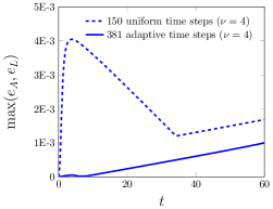
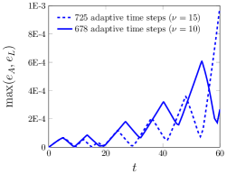
Figure 1: Left: The error as a function of time using a 150 uniform (dashed) and 381 adaptive (solid) time steps for a single vesicle with $\nu=4$. Even though the final errors are comparable, the adaptive time stepping scheme does not incur a large error near the start of the simulation. Right: The error as a function of time using 678 adaptive time steps for a single vesicle with $\nu=10$ (solid). The error happens to be decreasing near the time horizon, and this explains why the final error is not tight to the tolerance of 1E-3. This is in contrast to the simulation with $\nu=15$ (dashed) whose error is increasing near the time horizon, therefore, allowing the final error to be much tighter to the tolerance.

4.2 Two vesicles in a shear flow

We simulate two vesicles, each identical in shape to the last example, where the left vesicle’s center is slightly above the $x$-axis and the right vesicle’s center is on the $x$-axis. We allow for larger spatial errors by using $N=64$ points per vesicle, and the inter-vesicle interactions are accelerated with the fast multipole method [19]. One SDC correction is used, and the tolerance for the error in area and length at the time horizon is 1E-2. The time step size and several vesicle configurations are illustrated in Figs. 4–4 for different viscosity contrasts. Each vesicle is labelled with its viscosity contrast and marked with a single tracker point to help visualize the vesicle dynamics.

In Fig. 4, both the vesicles are tank-treading ($\nu=4$). We observe that the time step size is nearly constant except when the vesicles approach one another, and there, the time step size is reduced. The final error is 1.0E-2 which requires 545 accepted and 25 rejected time steps. In Fig. 4, one vesicle has a viscosity contrast $\nu=10$, while the other has a viscosity contrast $\nu=15$, which results in the this vesicle tumbling faster. The time step size is far less smooth, and the final error is 7.6E-3 which requires 975 accepted and 315 rejected time steps. Finally, in Fig. 4, one vesicle is tumbling ($\nu=10$), while the other is tank-treading ($\nu=4$). We see that the time step size is small when the tumbling vesicle has regions of high curvature, and when the vesicles are close. The final error is 1.0E-2 which requires 752 accepted and 158 rejected time steps.

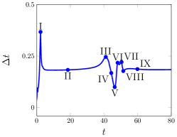
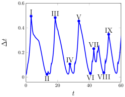
Figure 2: Two tank-treading vesicles ($\nu=4$). Left: The time step size taken to achieve the desired tolerance 1.0E-2 at the time horizon. The actual final error is 1.0E-2. Right: The vesicle configuration at the indicated labels.

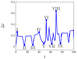
Figure 3: Two tumbling vesicles ($\nu=10$ and $\nu=15$). Left: The time step size taken to achieve the desired tolerance 1.0E-2 at the time horizon. The actual final error is 7.6E-3. Right: The vesicle configuration at the indicated labels. The vesicles are labelled with their viscosity contrast.

Figure 4: One tumbling vesicle ($\nu=10$) and one tank-treading vesicle ($\nu=4$). Left: The time step size taken to achieve the desired tolerance 1.0E-2 at the time horizon. The actual final error is 1.0E-2. Right: The vesicle configuration at the indicated labels. The vesicles are labelled with their viscosity contrast.

5 Conclusion

In this paper, we have extended our work on adaptive high-order time integrators for vesicle suspensions [9] to suspensions that include viscosity contrast. We have tested a second-order adaptive time integrator on two different suspensions with varying viscosity contrasts. Future work includes spatial adaptivity and implementing the presented results to three dimensions.

References

- Kraus et al. [1996] Kraus, M., Wintz, W., Seifert, U., Lipowsky, R.. Fluid Vesicles in Shear Flow. Physical Review Letter 1996;77(17):3685–3688.
- Seifert [1997] Seifert, U.. Configurations of fluid membranes and vesicles. Advances in Physics 1997;46:13–137.
- Sackmann [1996] Sackmann, E.. Supported membranes: Scientific and practical applications. Science 1996;271:43–48.
- Noguchi and Gompper [2005] Noguchi, H., Gompper, D.G.. Shape transitions of fluid vesicles and red blood cells in capillary flows. Proceedings Of The National Academy Of Sciences Of The United States Of America 2005;102:14159–14164.
- Pozrikidis [1990] Pozrikidis, C.. The Axisymmetric Deformation Of A Red Blood Cell In Uniaxial Straining Stokes Flow. Journal of Fluid Mechanics 1990;216:231–254.
- Ghigliotti et al. [2011] Ghigliotti, G., Rahimian, A., Biros, G., Misbah, C.. Vesicle Migration and Spatial Organization Driven by Flow Line Curvature. Physical Review Letters 2011;106:028101.
- Kaoui et al. [2011] Kaoui, B., Tahiri, N., Biben, T., Ez-Zahraouy, H., Benyoussef, A., Biros, G., et al. What Dictates Red Blood Cell Shapes and Dynamics in the Microvasculature? Physical Review E 2011;:1–11.
- Misbah [2006] Misbah, C.. Vacillating Breathing and Tumbling of Vesicles under Shear Flow. Physical Review Letters 2006;96(2).
- Quaife and Biros [2014a] Quaife, B., Biros, G.. Adaptive Time Stepping for Vesicle Simulations. arxiv 2014a;1405.6621.
- Dutt et al. [2000] Dutt, A., Greengard, L., Rokhlin, V.. Spectral Deferred Correction Methods for Ordinary Differential Equations. BIT Numerical Mathematics 2000;40:241–266.
- Minion [2003] Minion, M.L.. Semi-Implicit Spectral Deferred Correction Methods for Ordinary Differential Equations. Communications in Mathematical Sciences 2003;1(3):471–500.
- Christlieb et al. [2014] Christlieb, A.J., MacDonald, C.B., Ong, B.W., Spiteri, R.J.. Revisionist Integral Deferred Correction with Adaptive Step-Size Control. arxiv 2014;1310.6331v2.
- Huang et al. [2006] Huang, J., Lai, M.C., Xiang, Y.. An Integral Equation Method for Epitaxial Step-flow Growth Simulations. Journal of Computational Physics 2006;216:724–743.
- Rahimian et al. [2010] Rahimian, A., Veerapaneni, S.K., Biros, G.. Dynamic simulation of locally inextensible vesicles suspended in an arbitrary two-dimensional domain, a boundary integral method. Journal of Computational Physics 2010;229:6466–6484.
- Pozrikidis [1992] Pozrikidis, C.. Boundary Integral and Singularity Methods for Linearized Viscous Flow. New York, NY, USA: Cambridge University Press; 1992.
- Veerapaneni et al. [2009] Veerapaneni, S.K., Gueyffier, D., Zorin, D., Biros, G.. A boundary integral method for simulating the dynamics of inextensible vesicles suspended in a viscous fluid in 2D. Journal of Computational Physics 2009;228(7):2334–2353.
- Quaife and Biros [2014b] Quaife, B., Biros, G.. High-volume fraction simulations of two-dimensional vesicle suspensions. Journal of Computational Physics 2014b;274:245–267.
- Hairer et al. [1993] Hairer, E., Wanner, G., Nrsett, S.P.. Solving Ordinary Differential Equations I: Nonstiff Problems. Springer; 1993.
- Greengard and Rokhlin [1987] Greengard, L., Rokhlin, V.. A Fast Algorithm for Particle Simulations. Journal of Computational Physics 1987;73:325–348.