Proceedings of the Second Annual LHCP LHCB-PROC-2014-036

$C\!P$ violation in $B^{0}_{\mathrm{s}}$ decays at LHCb

Sean Benson

CERN, Geneva, Switzerland.

ABSTRACT

Latest LHCb measurements of $C\!P$ violation in the interference between mixing and decay are presented based on $pp$ collision data collected during LHC Run I, corresponding to an integrated luminosity of 3.0$\mbox{\,fb}^{-1}$. Approximately $27\,000$ $B^{0}_{\mathrm{s}}\to{\mathrm{J}\mskip-3.0mu/\mskip-2.0mu\psi\mskip 2.0mu}\pi^{+}\pi^{-}$ signal events are used to make what is at the moment the most precise single measurement of the $C\!P$-violating phase in $\mathrm{b}\to c\overline{}c\mathrm{s}$ transitions, $\phi_{\rm s}^{c\overline{}c\mathrm{s}}=0.070\pm 0.068\mathrm{(stat)}\pm 0.008\mathrm{(syst)}$$\rm\,rad$. The most accurate measurement of the $C\!P$-violating phase in $\mathrm{b}\to\mathrm{s}\overline{}\mathrm{s}\mathrm{s}$ transitions, $\phi_{\rm s}^{\mathrm{s}\overline{}\mathrm{s}\mathrm{s}}$, is found from approximately $4\,000$ $B^{0}_{\mathrm{s}}\to\phi\phi$ signal events to be $\phi_{\rm s}^{\mathrm{s}\overline{}\mathrm{s}\mathrm{s}}=-0.17\pm 0.15\mathrm{(stat)}\pm 0.03\mathrm{(syst)}$$\rm\,rad$.

PRESENTED AT

The Second Annual Conference

on Large Hadron Collider Physics

Columbia University, New York, U.S.A

June 2-7, 2014

1 Introduction

Efforts to measure mixing-induced $C\!P$ violation in the $B^{0}_{\mathrm{s}}$ system have mainly focused on the $B^{0}_{\mathrm{s}}\to{\mathrm{J}\mskip-3.0mu/\mskip-2.0mu\psi\mskip 2.0mu}\phi$ decay, utilising angular observables to disentangle the $C\!P$-odd and $C\!P$-even components. This then allows for the $C\!P$-violating phase, $\phi_{\rm s}^{c\overline{}c\mathrm{s}}$, to be measured. In the Standard Model, $\phi_{\rm s}^{c\overline{}c\mathrm{s}}\approx-2\beta_{s}=2arg(-V_{ts}V_{tb}^{*}/V_{cs}V_{cb}^{*})$ [1, 2, 3]. The Standard Model prediction for $\phi_{\rm s}^{c\overline{}c\mathrm{s}}$ has been obtained from global fits to experimental data yielding a value of $-0.036\pm 0.002$ $\rm\,rad$ [4, 5, 6]. There are however many New Physics theories that provide additional contributions to $B^{0}_{\mathrm{s}}$ mixing diagrams which alter this value [7, 8]. The addition of the ${B^{0}_{\mathrm{s}}\!\to{\mathrm{J}\mskip-3.0mu/\mskip-2.0mu\psi\mskip 2.0mu}\pi^{+}\pi^{-}}$ decay allows for an independent determination of $\phi_{\rm s}^{c\overline{}c\mathrm{s}}$.

The $C\!P$-violating phase measured in the $B^{0}_{\mathrm{s}}\to\phi\phi$ decay results from $\mathrm{b}\to\mathrm{s}\overline{}\mathrm{s}\mathrm{s}$ transitions and is therefore expected to be close to zero in the Standard Model due to the effective cancellation of the $C\!P$-violating weak phase between the $B^{0}_{\mathrm{s}}$ mixing diagrams and the penguin decay diagrams [9, 10]. Calculations using QCD factorisation provide an upper limit of 0.02$\rm\,rad$ for $|\phi_{\rm s}^{\mathrm{s}\overline{}\mathrm{s}\mathrm{s}}|$ [11, 12].

The following sections summarise updated measurements of the $C\!P$-violating weak phases in $\mathrm{b}\to c\overline{}c\mathrm{s}$ and $\mathrm{b}\to\mathrm{s}\overline{}\mathrm{s}\mathrm{s}$ transitions from the full LHCb Run I dataset of 3.0$\mbox{\,fb}^{-1}$, using $B^{0}_{\mathrm{s}}\to({\mathrm{J}\mskip-3.0mu/\mskip-2.0mu\psi\mskip 2.0mu}\to\mu^{+}\mu^{-})\pi^{+}\pi^{-}$ and $B^{0}_{\mathrm{s}}\to(\phi\to\mathrm{K}^{+}\mathrm{K}^{-})\;(\phi\to\mathrm{K}^{+}\mathrm{K}^{-})$ decays, respectively [13, 14].

2 The $\mathbf{B^{0}_{\mathrm{s}}\to{\mathrm{J}\mskip-3.0mu/\mskip-2.0mu\psi\mskip 2.0mu}\pi\pi}$ analysis

Previous analyses measuring $C\!P$ violation in $\mathrm{b}\to c\overline{}c\mathrm{s}$ transitions have been made using LHCb data collected in 2011, consisting of 1.0$\mbox{\,fb}^{-1}$, where the combined measurement of the $C\!P$-violating phase, $\phi_{\rm s}^{c\overline{}c\mathrm{s}}$, was found to be $0.01\pm 0.07\mathrm{(stat)}\pm 0.01\mathrm{(syst)}\rm\,rad$ [15, 16]. While previous analyses have used the measured result that the two-pion invariant mass spectrum is almost entirely $C\!P$-odd [17], the updated result presented here [13], uses $27\,100\pm 200$ signal events and incorporates an amplitude analysis that avoids assumptions on the $C\!P$ content.

Figure 1 shows the four-particle invariant mass range, $m({\mathrm{J}\mskip-3.0mu/\mskip-2.0mu\psi\mskip 2.0mu}\pi^{+}\pi^{-})$, from which the shape of the combinatorial background component is determined. For the $C\!P$ violation measurement, events in the range $|m({\mathrm{J}\mskip-3.0mu/\mskip-2.0mu\psi\mskip 2.0mu}\pi^{+}\pi^{-})-m_{B^{0}_{\mathrm{s}}}|<20{\mathrm{\,Me\kern-1.00006ptV\!/}c^{2}}$ are taken, such that only the $B^{0}_{\mathrm{s}}$ signal and combinatorial background components are present, where $m_{B^{0}_{\mathrm{s}}}$ is the PDG $B^{0}_{\mathrm{s}}$ mass. The $B^{0}_{\mathrm{s}}\to{\mathrm{J}\mskip-3.0mu/\mskip-2.0mu\psi\mskip 2.0mu}\pi^{+}\pi^{-}$ component is modelled with a double Crystal Ball function [18], with the combinatorial background modelled with an exponential.

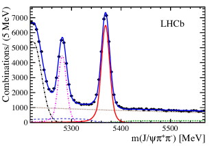
Figure 1: Distribution of the ${\mathrm{J}\mskip-3.0mu/\mskip-2.0mu\psi\mskip 2.0mu}\pi^{+}\pi^{-}$ invariant mass. Data are represented by black markers, the dotted magenta and solid red lines denote the $B^{0}\to{\mathrm{J}\mskip-3.0mu/\mskip-2.0mu\psi\mskip 2.0mu}\pi^{+}\pi^{-}$ and $B^{0}_{\mathrm{s}}\to{\mathrm{J}\mskip-3.0mu/\mskip-2.0mu\psi\mskip 2.0mu}\pi^{+}\pi^{-}$ fit components, respectively. The dotted brown line and the blue solid line represent the combinatorial background and the total fit, respectively. The reflections from $B^{0}\to{\mathrm{J}\mskip-3.0mu/\mskip-2.0mu\psi\mskip 2.0mu}\mathrm{K}^{+}\pi^{-}$ and $B^{+}\to{\mathrm{J}\mskip-3.0mu/\mskip-2.0mu\psi\mskip 2.0mu}h^{+}$ decays are given by the dotted black and green lines, respectively, and the dashed blue line represents the sum of the $B^{0}_{\mathrm{s}}\to{\mathrm{J}\mskip-3.0mu/\mskip-2.0mu\psi\mskip 2.0mu}\eta^{\prime}$, $B^{0}_{\mathrm{s}}\to{\mathrm{J}\mskip-3.0mu/\mskip-2.0mu\psi\mskip 2.0mu}(\phi\to\pi^{+}\pi^{-}\pi^{0})$, and $\Lambda_{\mathrm{b}}\to{\mathrm{J}\mskip-3.0mu/\mskip-2.0mu\psi\mskip 2.0mu}\mathrm{K}^{-}p$ reflections.

In order to measure $C\!P$ violation an un-binned maximum-likelihood fit is performed to the invariant mass, $m({\mathrm{J}\mskip-3.0mu/\mskip-2.0mu\psi\mskip 2.0mu}\pi^{+}\pi^{-})$, the $\pi^{+}\pi^{-}$ invariant mass, $m(\pi^{+}\pi^{-})$, the three helicity angles defined in Ref. [13], $\Omega\in\{\theta_{\pi\pi},\theta_{{\mathrm{J}\mskip-3.0mu/\mskip-2.0mu\psi\mskip 2.0mu}},\chi\}$ and the decay time, $t$. The total decay rates for the $B^{0}_{\mathrm{s}}\to{\mathrm{J}\mskip-3.0mu/\mskip-2.0mu\psi\mskip 2.0mu}\pi^{+}\pi^{-}$ and $\kern 1.79993pt\overline{\kern-1.79993ptB}{}^{0}_{\mathrm{s}}\to{\mathrm{J}\mskip-3.0mu/\mskip-2.0mu\psi\mskip 2.0mu}\pi^{+}\pi^{-}$ decays, denoted by $\Gamma(t)$ and $\overline{\Gamma}(t)$ respectively, can be written as

$$\Gamma(t) =e^{-\Gamma_{\mathrm{s}}t}\left(\frac{|\mathcal{A}|^{2}+|\overline{\mathcal{A}}|^{2}}{2}\cosh\frac{\Gamma_{\mathrm{s}}t}{2}+\frac{|\mathcal{A}|^{2}-|\overline{\mathcal{A}}|^{2}}{2}\cos(\Delta m_{\mathrm{s}}t)\right.$$

$$\left.-\Re(\mathcal{A}^{*}\overline{\mathcal{A}})\sinh\frac{\Gamma_{\mathrm{s}}t}{2}-\Im(\mathcal{A}^{*}\overline{\mathcal{A}})\sin(\Delta m_{\mathrm{s}}t)\right),$$ (1)

$$\overline{\Gamma}(t) =|p/q|^{2}e^{-\Gamma_{\mathrm{s}}t}\left(\frac{|\mathcal{A}|^{2}+|\overline{\mathcal{A}}|^{2}}{2}\cosh\frac{\Gamma_{\mathrm{s}}t}{2}-\frac{|\mathcal{A}|^{2}-|\overline{\mathcal{A}}|^{2}}{2}\cos(\Delta m_{\mathrm{s}}t)\right.$$

$$\left.-\Re(\mathcal{A}^{*}\overline{\mathcal{A}})\sinh\frac{\Gamma_{\mathrm{s}}t}{2}+\Im(\mathcal{A}^{*}\overline{\mathcal{A}})\sin(\Delta m_{\mathrm{s}}t)\right),$$ (2)

where $\Gamma_{\mathrm{s}}\equiv(\Gamma_{\rm L}+\Gamma_{\rm H})/2$ is the average decay rate, $\Delta\Gamma_{\mathrm{s}}\equiv\Gamma_{\rm L}-\Gamma_{\rm H}$ is the decay rate difference and $\Delta m_{\mathrm{s}}$ is the oscillation frequency of the $B^{0}_{\mathrm{s}}$ system. The decay amplitudes are defined as $\mathcal{A}=\sum_{i}A_{i}$ and $\overline{\mathcal{A}}=\sum_{i}\lambda_{i}A_{i}$, where $\lambda_{i}\equiv(q/p)(\overline{A}_{i}/A_{i})$, $A_{i}$ and $\overline{A}_{i}$ are the amplitudes of $B^{0}_{\mathrm{s}}$ mesons and $\kern 1.79993pt\overline{\kern-1.79993ptB}{}^{0}_{\mathrm{s}}$ mesons to the final state, $i$, at $t=0$, and the complex parameters, $q$ and $p$, relate the flavour eigenstates to the mass eigenstates of the $B^{0}_{\mathrm{s}}$ system at $t=0$. The full helicity dependence of the amplitudes on the two-pion invariant mass and helicity angles is provided in Ref. [19]. The probability density function (PDF) includes detector resolution and acceptance effects. The complete PDF is factorised to separate the ${\mathrm{J}\mskip-3.0mu/\mskip-2.0mu\psi\mskip 2.0mu}\pi^{+}\pi^{-}$ invariant mass from the other observables. The values of $\Gamma_{\mathrm{s}}$, $\Delta\Gamma_{\mathrm{s}}$ and $\Delta m_{\mathrm{s}}$ are constrained to LHCb measurements [15, 20].

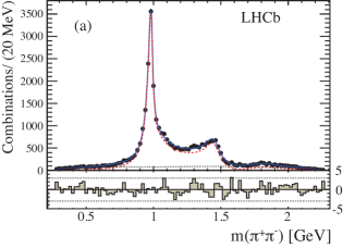
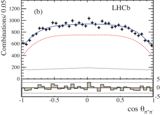
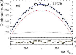
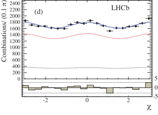
Figure 2: Projections of (a) $m(\pi^{+}\pi^{-})$, (b) $\cos\theta_{\pi\pi}$, (c) $\cos\theta_{{\mathrm{J}\mskip-3.0mu/\mskip-2.0mu\psi\mskip 2.0mu}}$, and (d) $\chi$. Data are shown by black markers, the total fit, signal and combinatorial background components are given by the solid blue line, dashed red line, and dotted black lines respectively.

It can be seen from Eqs. 1 and 2 that knowledge of the initial flavour of the $B^{0}_{\mathrm{s}}$ meson at production provides extra sensitivity to $C\!P$ violation. At LHCb, so-called flavour tagging is achieved through the use of the algorithms described in Refs. [15, 21]. This analysis uses both the opposite side (OS) and same side kaon (SSK) flavour taggers. The OS flavour tagging algorithm [22] makes use of the $\overline{}\mathrm{b}(\mathrm{b})$-quark produced in association with the signal $\mathrm{b}(\overline{}\mathrm{b})$-quark. The predicted probability of an incorrect flavour assignment, $\omega$, is determined for each event by a neural network that is calibrated using $B^{+}\to{\mathrm{J}\mskip-3.0mu/\mskip-2.0mu\psi\mskip 2.0mu}\mathrm{K}^{+}$, $B^{+}\to{{D}^{0}}\pi^{+}$, $B^{0}\to{\mathrm{J}\mskip-3.0mu/\mskip-2.0mu\psi\mskip 2.0mu}{\mathrm{K}^{*0}}$, $B^{0}\to{{D}^{*-}_{\mathrm{s}}}\mu^{+}{{\nu}_{\mu}}$, and $B^{0}_{\mathrm{s}}\to{{D}^{-}_{\mathrm{s}}}\pi^{+}$ data as flavour specific control modes. Details of the calibration procedure can be found in Ref. [15]. When a signal $B^{0}_{\mathrm{s}}$ meson is formed, an associated $\mathrm{s}$-quark is produced in the fragmentation that forms a charged kaon around 50 % of the time, The aforementioned charged kaon is likely to originate close to the $B^{0}_{\mathrm{s}}$ meson production point. The kaon charge therefore allows for the identification of the flavour of the signal $B^{0}_{\mathrm{s}}$ meson. This principle is exploited by the SSK flavour tagging algorithm [21]. The overall tagging power, calculated as $\epsilon_{\rm tag}(1-2\omega_{\rm avg})^{2}$, is found to be $(3.89\pm 0.25)\,\%$, where $\epsilon_{\rm tag}$ is the tagging efficiency, and $\omega_{\rm avg}$ is the average wrong-tag probability.

Figure 2 shows the projections of the two-pion invariant mass and the helicity angles. Good fit quality is seen showing that the complex $m(\pi^{+}\pi^{-})$ spectrum comprising of the $f_{0}(980)$, $f_{0}(1500)$, $f_{0}(1790)$, $f_{2}(1270)$, and $f_{2}^{\prime}(1525)$ resonances and associated interferences is understood. Efficiencies as a function of $m(\pi^{+}\pi^{-})$ and $\Omega$ are obtained from simulated events. The background distributions of the helicity angles are taken as the sum of the individual contributions and are parameterised as described in Ref. [23].

Figure 3 shows the projection of the $B^{0}_{\mathrm{s}}$ decay time integrated over all other observables, for events inside a 40${\mathrm{\,Me\kern-1.00006ptV\!/}c^{2}}$ window centred on the PDG $B^{0}_{\mathrm{s}}$ mass. The decay time acceptance is obtained from $B^{0}\to{\mathrm{J}\mskip-3.0mu/\mskip-2.0mu\psi\mskip 2.0mu}{\mathrm{K}^{*0}}$ events. The decay time resolution makes use of the per-event decay time error which is obtained from the kinematics of the candidate in question and is used in a triple-Gaussian model, after calibration using prompt ${\mathrm{J}\mskip-3.0mu/\mskip-2.0mu\psi\mskip 2.0mu}\to\mu^{+}\mu^{-}$ candidates.

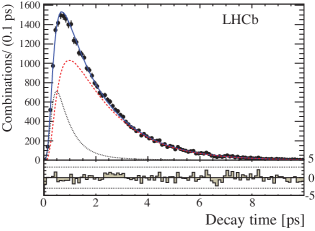
Figure 3: Decay time distribution of $B^{0}_{\mathrm{s}}\to{\mathrm{J}\mskip-3.0mu/\mskip-2.0mu\psi\mskip 2.0mu}\pi^{+}\pi^{-}$ candidates. Data are shown by black markers, the total fit, signal and combinatorial background components are given by the solid blue line, dashed red line, and dotted black lines respectively.

The background distribution is described using like-sign ${\pi^{\pm}}{\pi^{\pm}}$ candidates to obtain the parameters of a double exponential distribution combined with an acceptance function of the form $[a(t-t_{0})]^{n}/(1+[a(t-t_{0})]^{n})\times(1+\beta t+\beta_{2}t^{2})$, where $a,\,t_{0},\,n,\,\beta$ and $\beta_{2}$ are parameters to be fitted.

The dominant contributions to the systematic uncertainty are found to be from the production asymmetry and the models used to parameterise the resonances in the $m(\pi^{+}\pi^{-})$ spectrum. The former is accounted for by multiplying $\overline{\Gamma}(t)$ by the $B^{0}_{\mathrm{s}}$/$\kern 1.79993pt\overline{\kern-1.79993ptB}{}^{0}_{\mathrm{s}}$ production ratio, $R_{p}=(1.00\pm 0.05)$ [24] and varying $R_{p}$ within the associated error. The uncertainty on the resonance model arises from the addition of a $\rho(770)$ component, even though this component is forbidden by isospin conservation. The uncertainties on the $C\!P$-violating phase from these sources are 0.006$\rm\,rad$ in both cases. The uncertainties on the direct $C\!P$ violation parameter from these sources are 0.002 and 0.010, respectively.

The result of the measurement of the weak phase $\phi_{s}$ in the ${B^{0}_{\mathrm{s}}\!\to{\mathrm{J}\mskip-3.0mu/\mskip-2.0mu\psi\mskip 2.0mu}\pi^{+}\pi^{-}}$ decay is found to be $\phi_{s}=0.070\pm 0.068\mathrm{(stat)}\pm 0.008$$\rm\,rad$ [13]. The direct $C\!P$ violation parameter, $|\lambda|$, is measured to be $0.89\pm 0.05\mathrm{(stat)}\pm 0.01\mathrm{(syst)}$ [13] (note that a value of unity signifies no direct $C\!P$ violation). This result is more precise than the previous measurement using 1.0$\mbox{\,fb}^{-1}$ of LHCb data and is the most accurate single measurement of the $C\!P$-violating phase in $\mathrm{b}\to c\overline{}c\mathrm{s}$ transitions.

3 The $\mathbf{{B^{0}_{\mathrm{s}}\!\to\phi\phi}}$ Analysis

The ${B^{0}_{\mathrm{s}}\!\to\phi\phi}$ decay is an example of a flavour changing neutral current (FCNC) decay and as such, may only proceed via penguin diagrams in the Standard Model. The most recent analysis builds on the previous first measurement of the $C\!P$-violating phase [25], in addition to the measurement of the triple product asymmetries [26] using 1.0$\mbox{\,fb}^{-1}$ of LHCb data. A total of $4000$ signal candidates are observed through a multivariate selection to distinguish signal from background. Figure 4 shows the $\mathrm{K}^{+}\mathrm{K}^{-}\mathrm{K}^{+}\mathrm{K}^{-}$ invariant mass after all selections have been applied.

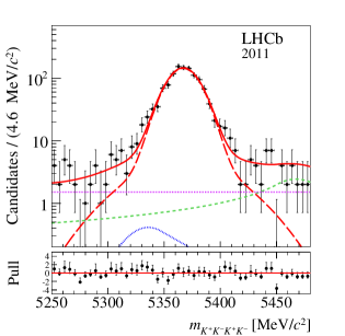
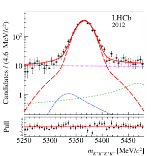
Figure 4: Four-kaon invariant mass distributions for the (left) 2011 and (right) 2012 datasets. Data are represented by black markers. Superimposed are the results of the total fit (red solid line), the ${B^{0}_{\mathrm{s}}\!\to\phi\phi}$ (red long dashed), the $B^{0}\to\phi{\mathrm{K}^{*0}}$ (blue dotted), the $\Lambda_{\mathrm{b}}\to\phi p\mathrm{K}^{-}$ (green short-dashed), and the combinatoric (purple dotted) fit components.

As in the case of the ${B^{0}_{\mathrm{s}}\!\to{\mathrm{J}\mskip-3.0mu/\mskip-2.0mu\psi\mskip 2.0mu}\pi^{+}\pi^{-}}$ analysis, a maximum log-likelihood fit is then performed to the three helicity angles and to the decay time. The ${B^{0}_{\mathrm{s}}\!\to\phi\phi}$ decay is a $P\to VV$ decay, where $P$ denotes a pseudoscalar and $V$ a vector meson. However, due to the proximity of the $\phi$ resonance to that of the $f_{0}(980)$, there will also be contributions from $S$-wave ($P\to V\kern-1.00006ptS$) and double $S$-wave ($P\to S\kern-1.00006ptS$) processes, where $S$ denotes a spin-0 meson or a pair of non-resonant kaons. Thus the total amplitude is a coherent sum of $P$-, $S$-, and double $S$-wave processes, and is accounted for during fitting by making use of the different functions of the helicity angles associated with these terms. The functional form of the PDF in terms of the decay time and helicity angles is given in Ref. [14]. The parameters of interest are the $C\!P$ violation parameters ($\phi_{\rm s}^{\mathrm{s}\overline{}\mathrm{s}\mathrm{s}}$ and $|\lambda|$), the polarisation amplitudes ($|A_{0}|^{2}$, $|A_{\perp}|^{2}$, $|A_{S}|^{2}$, and $|A_{SS}|^{2}$), and the $C\!P$-conserving strong phases ($\delta_{1}$, $\delta_{2}$, $\delta_{S}$, and $\delta_{SS}$). The $P$-wave amplitudes are defined such that $|A_{0}|^{2}+|A_{\perp}|^{2}+|A_{\parallel}|^{2}=1$, hence only two are free parameters.

Flavour tagging is achieved with the same algorithms as used for the measurement of $\phi_{\rm s}^{c\overline{}c\mathrm{s}}$ in the ${B^{0}_{\mathrm{s}}\!\to{\mathrm{J}\mskip-3.0mu/\mskip-2.0mu\psi\mskip 2.0mu}\pi^{+}\pi^{-}}$ decay. The efficiencies as a function of decay angles are accounted for with simulated ${B^{0}_{\mathrm{s}}\!\to\phi\phi}$ events that have been subjected to the same selection requirements as used for the data sample. The decay time acceptance is accounted for with the $B^{0}_{\mathrm{s}}\to{{D}^{-}_{\mathrm{s}}}\pi^{+}$ control mode, that is re-weighted according to the final state particle transverse momentum. The same decay time biasing selections as used to select the ${B^{0}_{\mathrm{s}}\!\to\phi\phi}$ decay are applied in addition to a requirement that the ${D}^{-}_{\mathrm{s}}$ decay time be less than $1{\rm\,ps}$, to enforce topological similarity to the ${B^{0}_{\mathrm{s}}\!\to\phi\phi}$ decay. Decay time resolution is accounted for with a per-event decay time error, used in association with a Gaussian model after having first been calibrated using simulated events.

The 2011 and 2012 data samples are assigned independent signal weights, decay time and angular acceptances, in addition to separate Gaussian constraints to the decay time resolution parameters. The value of the $B^{0}_{\mathrm{s}}$-$\kern 1.79993pt\overline{\kern-1.79993ptB}{}^{0}_{\mathrm{s}}$ oscillation frequency is constrained to the LHCb measured value  [20]. The values of the decay width and decay width difference are constrained to the LHCb measured values of $\Gamma_{\mathrm{s}}=0.661\pm 0.004\mathrm{(stat)}\pm 0.006\mathrm{(syst)}$${\rm\,ps^{-1}}$ and $\Delta\Gamma_{\mathrm{s}}=0.106\pm 0.011\mathrm{(stat)}\pm 0.007\mathrm{(syst)}$${\rm\,ps^{-1}}$, respectively [15]. The Gaussian constraints applied to the $\Gamma_{\mathrm{s}}$ and $\Delta\Gamma_{\mathrm{s}}$ parameters use the combination of the measured values from $B^{0}_{\mathrm{s}}\to{\mathrm{J}\mskip-3.0mu/\mskip-2.0mu\psi\mskip 2.0mu}\mathrm{K}^{+}\mathrm{K}^{-}$ and $B^{0}_{\mathrm{s}}\to{\mathrm{J}\mskip-3.0mu/\mskip-2.0mu\psi\mskip 2.0mu}\pi^{+}\pi^{-}$ decays. Constraints are therefore applied taking into account a correlation of $0.1$ for the statistical uncertainties [15]. The systematic uncertainties are taken to be uncorrelated between the $B^{0}_{\mathrm{s}}\to{\mathrm{J}\mskip-3.0mu/\mskip-2.0mu\psi\mskip 2.0mu}\mathrm{K}^{+}\mathrm{K}^{-}$ and $B^{0}_{\mathrm{s}}\to{\mathrm{J}\mskip-3.0mu/\mskip-2.0mu\psi\mskip 2.0mu}\pi^{+}\pi^{-}$ decay modes.

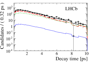
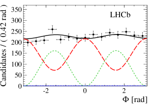
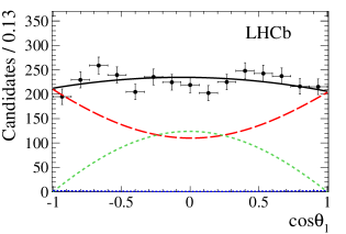
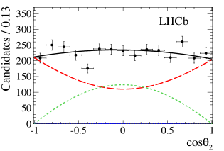
Figure 5: One-dimensional projections of the $B^{0}_{\mathrm{s}}\to\phi\phi$ fit for (top-left) decay time with binned acceptance, (top-right) helicity angle $\Phi$ and (bottom-left and bottom-right) cosine of the helicity angles $\theta_{1}$ and $\theta_{2}$. The background-subtracted data are marked as black points, while the black solid lines represent the projections of the best fit. The $C\!P$-even $P$-wave, the $C\!P$-odd $P$-wave and $S$-wave combined with double $S$-wave components are shown by the red long dashed, green short dashed and blue dotted lines, respectively.

Figure 5 shows the projections on to the helicity angles and decay time, the fit to which yields $C\!P$ violation parameters of $\phi_{\rm s}^{\mathrm{s}\overline{}\mathrm{s}\mathrm{s}}=-0.17\pm 0.15\mathrm{(stat)}\pm 0.03\mathrm{(syst)}$$\rm\,rad$ and $|\lambda|=1.04\pm 0.07\mathrm{(stat)}\pm 0.03\mathrm{(syst)}$. Polarisation amplitudes are measured to be $|A_{0}|^{2}=0.364\pm 0.012\mathrm{(stat)}\pm 0.009\mathrm{(syst)}$ and $|A_{\perp}|^{2}=0.305\pm 0.013\mathrm{(stat)}\pm 0.005\mathrm{(syst)}$, where $|A_{\parallel}|^{2}$ is fixed such that the fractions of the $P$-wave sum to unity. In addition, the $S$-wave fractions are found to be consistent with a pure $P$-wave state.

A separate un-binned maximum log-likelihood fit is performed to the four-kaon mass in data samples that have been divided according to the sign of the $T$-odd observables, $U=\sin\Phi\cos\Phi$ and $V=\pm\sin\Phi$, where the positive sign is taken if $\cos\theta_{1}\cos\theta_{2}>0$ else the negative sign is used [27]. With such a fit, asymmetries can be measured in the $T$-odd observables, denoted $A_{U}$ and $A_{V}$, which provide a method of measuring $C\!P$ violation that does not require flavour tagging or knowledge of the decay time. These so-called triple product asymmetries are measured to be $A_{U}=-0.003\pm 0.017\mathrm{(stat)}\pm 0.006\mathrm{(syst)}$ and $A_{V}=-0.017\pm 0.017\mathrm{(stat)}\pm 0.006\mathrm{(syst)}$.

The dominant sources of systematic uncertainties are found to arise from the angular and decay time acceptances, which each contribute uncertainties of 0.02$\rm\,rad$ to the systematic uncertainty on $\phi_{\rm s}^{\mathrm{s}\overline{}\mathrm{s}\mathrm{s}}$. The mass model is also found to have a significant effect for the measurement of the triple product asymmetries.

4 Summary

The most accurate single measurement of $C\!P$ violation in $B^{0}_{\mathrm{s}}$ mixing has been presented using the full Run I dataset collected with the LHCb detector, corresponding to an integrated luminosity of 3.0$\mbox{\,fb}^{-1}$. The analysis of approximately $27,\,000$ ${B^{0}_{\mathrm{s}}\!\to{\mathrm{J}\mskip-3.0mu/\mskip-2.0mu\psi\mskip 2.0mu}\pi^{+}\pi^{-}}$ decays yields a measurement of $\phi_{\rm s}^{c\overline{}c\mathrm{s}}=0.070\pm 0.068\mathrm{(stat)}\pm 0.008\mathrm{(syst)}$$\rm\,rad$. The most precise measurement of the $C\!P$-violating phase in the ${B^{0}_{\mathrm{s}}\!\to\phi\phi}$ penguin decay is also presented, which is found to be $\phi_{\rm s}^{\mathrm{s}\overline{}\mathrm{s}\mathrm{s}}=-0.17\pm 0.15\mathrm{(stat)}\pm 0.03\mathrm{(syst)}$$\rm\,rad$. All results are consistent with Standard Model expectations. Statistical uncertainties are found to be dominant in all measurements of $C\!P$ violation, hence measurements with greater precision can be expected with the addition of Run II data.

References

[1]
S. Faller, R. Fleischer and T. Mannel,
Phys. Rev. D 79 (2009) 014005
[arXiv:0810.4248 [hep-ph]].
[2]
A. S. Dighe, I. Dunietz and R. Fleischer,
Eur. Phys. J. C 6 (1999) 647
[hep-ph/9804253].
[3]
I. Dunietz, R. Fleischer and U. Nierste,
Phys. Rev. D 63 (2001) 114015
[hep-ph/0012219].
[4]
J. Charles et al.,
Phys. Rev. D 84 (2011) 033005
[arXiv:1106.4041 [hep-ph]].
[5]
A. Lenz and U. Nierste,
JHEP 0706 (2007) 072
[hep-ph/0612167].
[6]
A. Lenz and U. Nierste,
arXiv:1102.4274 [hep-ph].
[7]
P. Ball and R. Fleischer,
Eur. Phys. J. C 48 (2006) 413
[hep-ph/0604249].
[8]
A. Lenz,
Phys. Rev. D 76 (2007) 065006
[arXiv:0707.1535 [hep-ph]].
[9]
M. Raidal,
Phys. Rev. Lett. 89 (2002) 231803
[hep-ph/0208091].
[10]
B. Bhattacharya, A. Datta, M. Duraisamy and D. London,
Phys. Rev. D 88 (2013) 1, 016007
[arXiv:1306.1911 [hep-ph]].
[11]
M. Bartsch, G. Buchalla and C. Kraus,
arXiv:0810.0249 [hep-ph].
[12]
H. Y. Cheng and C. K. Chua,
Phys. Rev. D 80 (2009) 114026
[arXiv:0910.5237 [hep-ph]].
[13]
R. Aaij et al. [LHCb Collaboration],
Phys. Lett. B 736 (2014) 186
[arXiv:1405.4140 [hep-ex]].
[14]
R. Aaij et al. [LHCb Collaboration],
arXiv:1407.2222 [hep-ex].
[15]
R. Aaij et al. [LHCb Collaboration],
Phys. Rev. D 87 (2013) 11, 112010
[arXiv:1304.2600 [hep-ex]].
[16]
R. Aaij et al. [LHCb Collaboration],
Phys. Lett. B 713 (2012) 378
[arXiv:1204.5675 [hep-ex]].
[17]
R. Aaij et al. [LHCb Collaboration],
Phys. Rev. D 86 (2012) 052006
[arXiv:1204.5643 [hep-ex]].
[18]
T. Skwarnicki,
DESY-F31-86-02 (1986).
[19]
L. Zhang and S. Stone,
Phys. Lett. B 719 (2013) 383
[arXiv:1212.6434].
[20]
R. Aaij et al. [LHCb Collaboration],
New J. Phys. 15 (2013) 053021
[arXiv:1304.4741 [hep-ex]].
[21]
R. Aaij et al. [LHCb Collaboration],
LHCb-CONF-2012-033 (2012).
[22]
R. Aaij et al. [LHCb Collaboration],
LHCb-CONF-2012-026 (2012).
[23]
R. Aaij et al. [LHCb Collaboration],
Phys. Rev. D 89 (2014) 092006
[arXiv:1402.6248 [hep-ex]].
[24]
E. Norrbin and R. Vogt,
CERN-99-09 (1999)
[hep-ph/0003056].
[25]
R. Aaij et al. [LHCb Collaboration],
Phys. Rev. Lett. 110 (2013) 24, 241802
[arXiv:1303.7125 [hep-ex]].
[26]
R. Aaij et al. [LHCb Collaboration],
Phys. Lett. B 713 (2012) 369
[arXiv:1204.2813 [hep-ex]].
[27]
M. Gronau and J. L. Rosner,
Phys. Rev. D 84 (2011) 096013
[arXiv:1107.1232 [hep-ph]].