Show Me the Money: Dynamic Recommendations for Revenue Maximization
Abstract
Recommender Systems (RS) play a vital role in applications such as e-commerce and on-demand content streaming. Research on RS has mainly focused on the customer perspective, i.e., accurate prediction of user preferences and maximization of user utilities. As a result, most existing techniques are not explicitly built for revenue maximization, the primary business goal of enterprises. In this work, we explore and exploit a novel connection between RS and the profitability of a business. As recommendations can be seen as an information channel between a business and its customers, it is interesting and important to investigate how to make strategic dynamic recommendations leading to maximum possible revenue. To this end, we propose a novel revenue model that takes into account a variety of factors including prices, valuations, saturation effects, and competition amongst products. Under this model, we study the problem of finding revenue-maximizing recommendation strategies over a finite time horizon. We show that this problem is NP-hard, but approximation guarantees can be obtained for a slightly relaxed version, by establishing an elegant connection to matroid theory. Given the prohibitively high complexity of the approximation algorithm, we also design intelligent heuristics for the original problem. Finally, we conduct extensive experiments on two real and synthetic datasets and demonstrate the efficiency, scalability, and effectiveness our algorithms, and that they significantly outperform several intuitive baselines.
1 Introduction
Fueled by online applications such as e-commerce (e.g., Amazon.com) and on-demand content streaming (e.g., Netflix), Recommender Systems (RS) have emerged as a popular paradigm and often as an alternative to search, for enabling customers to quickly discover needed items. Such systems use the feedback (e.g., ratings) received from users on the items they have bought or experienced to build profiles of users and items, which are then used to suggest new items that might be of interest [1]. The key technical problem on which most RS research has focused is rating prediction and rating-based top- recommendations: given all ratings observed so far, predict the likely ratings users would give unrated products. In practice, the data is huge, with typically hundreds of thousands of users and items, and is sparse, as users rate very few items. Major rating prediction techniques can be categorized into content-based and collaborative filtering (CF). The latter can be further divided into memory-based and model-based (cf. §2, also [1, 18, 26]). Here we simply note that for top- recommendations, a RS predicts ratings for all user-item pairs, and for each user, pushes the items with the highest predicted ratings as personalized recommendations.
The above account is a customer-centric view of RS, on which most existing research has focused. We also refer to it as rating-based recommendation. There is an equally important, complementary business-centric view. From a business viewpoint, the goal of a seller running a RS is to maximize profit or revenue. It is thus natural to ask: When a recommender system has choices of promising items but can only recommend up to items at a time, how should it make the selections to achieve better revenue? We refer to this as revenue-driven recommendation.
Top- rating-based recommendations are relevant to revenue, but the connection is weak and indirect: by suggesting to each user the items with highest predicted rating, the hope is to increase the chances that some of those items are bought, and there ends the connection. Clearly, there exists a gap: rating-based approaches ignores important monetary factors that are vital to users’ product adoption decisions, namely the price and whether such price would be considered acceptable to an individual. Naturally there exists inherent uncertainty in users’ purchase decisions due to people’s innate valuation [15], and thus successful revenue-driven recommendations must be aware of these monetary factors.
There has been some recent work on revenue-driven recommendations [6, 7, 3] (see §2 for more details). All these previous works focus on a static setting: generate a set of recommendations for various users for a given snapshot, corresponding to a specific time. This is limited because e-commerce markets are highly dynamic in nature. For example, the price of many products in Amazon has been found to change and fluctuate frequently [4, 2]. Therefore, narrowly focusing on just one snapshot is restrictive. Instead, it is necessary to be strategic about the recommendations rolled out in a short time period. For instance, suppose a product is scheduled to go on sale in the next few days, it would be wise to strategically postpone its recommendation to low-valuation users (those not willing to pay the original price) to the sale date, so as to increase the adoption probability. On the contrary, for high-valuation users (those willing to pay the original price), it is wiser to recommend it before the price drops. This illustrates that sellers may benefit from taking full advantage of known price information in near future. Thus, revenue-driven recommendations should be not only price-aware, but also sensitive to timing. As such, we focus on a dynamic setting where a strategic recommendation plan is rolled out over a time horizon for which pricing information is available (either deterministically or probabilistically). We note that by myopically repeating items, the static approaches can be used to roll out recommendations over a horizon; we will empirically compare the performance of such strategies with our solutions in §6.
The dynamic setting naturally leads to two more important aspects related to revenue: competition and repeated recommendations. Products in the same class (kind) provide similar functionalities to customers, and thus an individual is unlikely to purchase multiple of them at once. This signals competition and its implications for the actual revenue yielded by repeated recommendations cannot be ignored. For instance, iPhone 5S, Nokia 820, and Blackberry Z10 are all smartphones. While an individual may find them all appealing, she is likely to purchase at most one even if all three phones are suggested to her (potentially more than once) during a short time period. In addition, as observed recently [8], while moderate repeated recommendation may boost the ultimate chance of adoption, overly repeating could lead to boredom, or saturation. All these factors, not considered in previous work [6, 7, 3], call for careful modeling and a more sophisticated algorithmic framework.
Driven by the above, we pose the problem of designing recommendation strategies to maximize the seller’s expected revenue as a novel discrete optimization problem, named RevMax (for revenue maximization). Our framework allows any type of RS to be used, be it content-based, memory-based CF, or model-based CF. It takes prices as exogenous input to the RS, and nicely models adoption uncertainly by integrating the aforementioned factors: price, competition, and saturation (see §3 for a detailed justification and supporting literature). We show RevMax is NP-hard and develop an approximation algorithm (for a relaxed version) and fast greedy heuristics. To the best of our knowledge, no existing work on RS has a revenue model that incorporates the various factors captured by our revenue model. Furthermore, the discrete optimization problem proposed and the algorithmic solution framework designed in this work are unique and complement previous work nicely.
To summarize, we make the following contributions.
-
We propose a dynamic revenue model that accounts for time, price, saturation effects, and competition. Under this model, we propose RevMax, the problem of finding a recommendation strategy that maximizes the seller’s expected total revenue over a short time horizon. To the best of our knowledge, this framework is novel and unique.
-
We show that RevMax is NP-hard (§3) and its objective function is non-monotone and submodular (§4). By establishing a connection to matroids, a relaxed version of RevMax can be modeled as submodular function maximization subject to matroid constraints, enabling a local search algorithm with an approximation guarantee of , for any (§4).
-
Since the local search approximation algorithm is prohibitively expensive and not practical, we design several clever and scalable greedy heuristics for RevMax (§5).
-
We perform a comprehensive set of experiments on two real datasets (Amazon and Epinions) that we crawled, to show the effectiveness and efficiency of our algorithms. In particular, they significantly outperform natural baselines. We use the data to learn the various parameters used in the experiments (§6). We also show that our best algorithm, Global Greedy, scales to a (synthetically generated) dataset that is 2.5 times as large as Netflix, the largest publicly available ratings dataset.
-
We also discuss promising extensions to our framework in §7. In particular, we show that when exact price information is not available but only a price distribution is known, Taylor approximation can be employed for maximizing (approximate) expected total revenue.
2 Background and Related Work
The majority of the research in RS has focused on algorithms for accurately predicting user preferences and their utility for items in the form of ratings, from a set of observed ratings. As mentioned in §1, RS algorithms can be classified into content-based or collaborative filtering (CF) methods, with CF being further classified into memory-based or model-based [1]. The state-of-the-art is collaborative filtering using Matrix Factorization (MF), which combines good accuracy and scalability [18]. In MF, users and items are characterized by latent feature vectors inferred from ratings. More specifically, we learn for each user a vector and for each item a vector , such that for all observed ratings ( is the number of latent features). Training the model requires an appropriate loss function to measure the training error, so that using methods like stochastic gradient descent or alternating least squares, the latent feature vectors can be learned quickly in a few iterations [18]. The most common loss functions is RMSE [18]. For our purposes, existing MF methods can be used to compute predicted ratings accurately and efficiently, although our framework does permit the use of other methods. Recently, Koren [17] considers the drift in user interests and item popularity over time and proposes a temporal MF model to further improve accuracy. This model is for rating prediction and uses data spanning a long period, since drifts usually occur gradually, while our framework addresses dynamic recommendations over a short period and has a completely different objective (revenue).
Other related work of the customer-centric view includes [32, 31]. Zhao et al. [32] compute the time interval between successive product purchases and integrate it into a utility model for recommendations, with the idea of capturing the timing of recommendations well and increasing temporal diversity. Wang et al. [31] apply survival analysis to estimate from data the probability that a user will purchase a given product at a given time. It offers a way of modeling and computing adoption probability and is in this sense orthogonal to RevMax. We depart from these works by focusing on strategic recommendation plans for short-term for which price information is known and repeated purchase is rare, and formulating RevMax as a discrete optimization problem.
There has been some work on revenue-driven recommendations [6, 7, 3]. However, most of it deals with a static setting and is limited in several senses. Chen et al. [6] model adoption probabilities using purchase frequency and user similarity, and recommend each user -highest ranked items in terms of expected revenue (probability price). Important ingredients such as capacity constraints, competition, price fluctuations and saturation are all ignored. Consequently, their optimization can simply be solved independently for each user, without the combinatorial explosion inherent in our problem, which is far more challenging. It is also tied to memory-based RS (user similarity), whereas our approach is more generic and works for any type of RS. Das et al. [7] propose a simple profit model which predicts the adoption probability using the similarity between the user’s true ratings and the system prediction. It captures the trust between users and the RS, but does not take into account the fact that when the price or relevance of suggested items changes, user’s adoption probability ought to change too. Azaria et al. [3] model the probability of a movie being viewed based on its price and rank (from a black-box RS). Their setting is also static and focuses on movies only, which is not sufficient for most e-commerce businesses that sell a variety of products.
Static revenue-driven recommendation, on an abstract level, is related to generalized bipartite matching [10, 11]. The papers [23, 21] propose distributed solution frameworks to scale this up to massive datasets. They are substantially different from and orthogonal to ours as the focus is on distributed computation, still within a static setting. We defer detailed discussion to §3.
3 Revenue Maximization
The motivation for a dynamic view of revenue-based recommendations is twofold. First, prices change frequently, sometimes even on a daily basis, or several times a day in online marketplaces like Amazon [4, 2]. A static recommendation strategy is forced to be myopic and cannot take advantage of price fluctuations to choose the right times at which an item should be recommended. This shortcoming is glaring, since for product adoptions to occur, a user’s valuation of an item, i.e., the maximum amount of money she is willing to pay, must exceed the price. This is a well-known notion in economics literature [24, 28, 15]. And obviously, the optimal time in terms of extracting revenue is not necessarily when the price is at its peak or bottom! Therefore, only by incorporating time, we can design revenue-maximizing recommendations in a systematic, holistic, and principled way.
Second, we can recommend items strategically over a time horizon, possibly making some repetitions, to improve the chances that some items are eventually bought. However, this is delicate. Indiscriminate repeat recommendations can lead to saturation effects (boredom), turning off the user from the item or even costing her loyalty to the RS. Thus, we need to choose the timing of recommendations as well as their frequency and placement so as to maximize the expected revenue in the presence of saturation effects. These opportunities are simply not afforded when recommendations are made in a static, one-shot basis.
3.1 Problem Setting and Definition
We adopt a discrete time model to describe the dynamics of revenue in an e-commerce business. Let and be the set of users and items respectively, and define to be a short time horizon over which a business (or seller) plans a recommendation strategy. The seller may choose the granularity of time at her discretion. E.g., the granularity may be a day and the horizon may correspond to a week.
Naturally, items can be grouped into classes based on their features and functionalities, e.g., “Apple iPad Mini” and “Google Nexus 7” belong to class tablet, while “Samsung Galaxy S4” and “Google Nexus 5” belong to smartphone. Items in the same class offer a variety of options to customers and thus compete with each other, since from an economic point of view, it is unlikely for a person to adopt multiple products with similar functionality over a short time horizon. Thus in our model, we assume items within a class are competitive in the sense that their adoption by any user within is mutually exclusive.
In general, revenue to be expected from a recommendation depends mainly on two factors: the price of the item, and the probability that the user likes and then adopts the item at that price. The latter, as mentioned in §1, is in turn dependent on many factors, including but not restricted to, price. The former, price, is conceptually easier to model, and we suggest two alternatives. Both of the following essentially model prices to be exogenous to the RS, meaning, they are externally determined and provided to the RS. First, we can use an exact price model which assumes that for each item and time step , the exact value is known. Exact pricing is studied extensively in microeconomics theory. There is a well established theory for estimating future demand and supply, which are further used to derive future price in market equilibrium [30]. In practice, we also observe that retailers (both online and offline) do plan their pricing ahead of time (e.g., sales on Black Friday in the US and Boxing Day in Canada). Alternatively, in case prices are not completely known – which could be possible if the time of interest is too far into the future, or there isn’t sufficient data to determine a precise value – they can be modeled as random variables following a certain probability distribution. In other words, there is a price prediction model that produces a probability distribution associated with price. As we shall see shortly, the challenge of revenue maximization in RS remains in both exact price and random price models. In the bulk of this paper, we focus on the exact price model, but in §7, give insights on how the random price model can be incorporated into our framework.
It is well known that there is uncertainty in product adoption by users. Consider any user-item-time triple . We associate it with a (primitive) adoption probability , the probability that would purchase at time . Based on economics theory, buyers are rational and utility-maximizing [28, 24] and would prefer lower price for higher utility (of consuming a product). Rational agents are typically assumed to possess a private, internal valuation for a good, which is the maximum amount of money the buyer is willing to pay; furthermore, users are assumed to be price-takers who respond myopically to the prices offered to them, solely based on their privately-held valuations and the price offered. Both the internal private valuation assumption and the price taker assumption are standard in economics literature [28, 24]. Thus, though a lower price leads to a higher probability of adoption, it might not be optimal to recommend an item at its lowest price, since some buyers actually could be willing to pay more. In general, a seller may estimate the adoption probabilities using its own data and model, and the exact method used for estimating adoption probabilities is orthogonal to our framework. In §6, we give one method for estimating adoption probabilities from the real datasets Amazon and Epinions. We note that the above notion is “primitive” in the sense that it ignores the effect of competition and saturation, which will be captured in Definition 1.
Intuitively, the expected revenue yielded by recommending item to user at time is , if this recommendation is considered in isolation. However, competition and repeated suggestions make the expected revenue computation more delicate. We first formally define a recommendation strategy as a set of user-item-time triples , where means is recommended to at time . Let us next consider the effect of competition and repeated recommendations. Suppose suggests multiple items (possibly repeated) within a class to user , then the adoption decisions that a user makes at different times are interdependent in the following manner: The event that a user adopts an item at time is conditioned on not adopting any item from ’s class before, and once adopts , she will not adopt anything from that class again in the horizon (which, it may be recalled, is short in our model). This semantics intuitively captures competition effects.
As argued earlier, repeated suggestions may lead to a boost in adoption probability, but repeating too frequently may backfire, as people have a tendency to develop boredom, which can potentially cause devaluation in user preference [8, 16]. We call this saturation effect. This is undesirable in terms of revenue and thus the model should be saturation-aware. We discount the adoption probability by accounting for saturation, similar in spirit to [8]. The intuition is that the more often and more recently a user has been recommended an item or an item from the same class, the fresher her memory and consequently the more significant the devaluation. Let denote the class to which belongs. The memory of user on item at any time w.r.t. a recommendation strategy is
| (1) |
where is an indicator variable taking on if and otherwise. Also for all , , and . The discounting on adoption probability should reflect the fact that devaluation is monotone in memory. More specifically, given user , item , and time step , we define the saturation-aware adoption probability under a strategy as , where is the saturation factor of item . This effectively penalizes recommending the same class of items in (nearly) consecutive time steps. Smaller means greater saturation effect. corresponds to no saturation and corresponds to full saturation: any repetition immediately leads to zero probability. In principle, ’s can be learned from historical recommendation logs (cf. [8]).
Combining competition and saturation effects, we are now ready to define the strategy-dependent dynamic adoption probability. Basically, the dynamic adoption probability for later times depends on earlier times at which recommendations are made. Intuitively, is the probability that adopts at time and does not adopt any item from its class earlier, under the influence of .
Definition 1 (Dynamic Adoption Probability)
For any user , item , and time step , given a strategy , the dynamic adoption probability governed by is defined as follows:
| (2) |
Also, define whenever .
Example 1 (Dynamic Adoption Probability)
Suppose the strategy consists of , where , and for all three triples, the (primitive) adoption probability is . Then, , , and .
We next define the expected revenue of a recommendation strategy, as the expected amount of money the business (seller) can earn from recommendation-led adoptions by following the strategy.
Definition 2 (Revenue Function)
Given a set of users, a set of items, and time horizon , the expected revenue of any strategy is
| (3) |
where is defined in Definition 1.
The revenue maximization problem asks to find a strategy with maximum expected revenue, subject to the following two natural constraints: First, the display constraint, following standard practice, requires that no more than items be recommended to a user at a time. Second, as items all have limited quantities in inventory, we impose a capacity constraint: no item may be recommended to more than distinct users at any time, where is a number determined based on current inventory level and demand forecasting [25]. The intention is to avoid potential customer dissatisfaction caused by out-of-stock items. In general, can be somewhat higher than the actual inventory level, due to uncertainty in product adoption. We call a strategy valid if satisfies the following constraints: (i) for all and all , ; (ii) for all , .
Problem 1 (Revenue Maximization (RevMax))
Given a set of users, of items, time horizon , display limit ; for each , capacity , price , and saturation factor ; adoption probabilities for all , find the optimal valid recommendation strategy, i.e., .
3.2 Hardness of Revenue Maximization
As we will show shortly, RevMax is in general NP-hard. However, when , it is PTIME solvable since it can be cast as a special case of the maximum-weighted degree-constrained subgraph problem (Max-DCS) [10, 11]. In Max-DCS, we are given a graph , a weight for each edge , and a number for each node . The task is to find a subgraph of that has maximum weight and for each , it contains no more than edges incident to . The best known combinatorial algorithm for Max-DCS takes time [10, 11].
Given an instance of RevMax with , we create an instance of Max-DCS, by building a bipartite graph , where . We create one node per user, and per item. For each user-node , set , and for each item-node , set . There is an edge if and set the weight . It is easy to see the optimal subgraph in corresponds to the optimal strategy in . Thus, this special case of RevMax can be solved efficiently using known algorithms for Max-DCS.
We now show that the general RevMax is NP-hard. The reduction is from a restricted version of the Timetable-Design problem (RTD), which is NP-complete [13, 9], to the decision-version of RevMax (D-RevMax). An instance of the RTD problem consists of a set of craftsmen, a set of jobs, and a set of of hours, where . Each craftsman is available for a subset of hours, thus is the number of hours that is available. There is a function , such that specifies the number of hours craftsman is required to work on job . A craftsman is a -craftsman if . Furthermore, he is tight, if he is a -craftsman for some and is required to work on jobs, i.e., . In RTD, every craftsman is either a -craftsman or a -craftsman and is tight. A timetable is a function . It is feasible if all of the following hold:
-
1.
implies ;
-
2.
for each and there is at most one such that ;
-
3.
for each and there is at most one such that ; and
-
4.
for each pair there are exactly values of for which .
The task in RTD is to determine if a feasible timetable exists.
Theorem 1
Problem 1 (RevMax) is NP-hard.
Proof 3.2.
Given an instance of RTD, we create an instance of D-RevMax as follows. Craftsmen and hours in correspond to users and time steps in . For each job , create three items of class : . The subscripts correspond to the three hours in . For every item the capacity constraint is , i.e., , . The display constraint . Set price if , and otherwise. For user , item , and any time step , set . For every user , we create a unique expensive item and set for all time , where is an arbitrary number such that . For any time at which is unavailable, i.e., if , set and for all times at which is available, i.e., for , . Finally, let , i.e., the total number of unavailable hours of all craftsmen.
Claim: admits a recommendation strategy of expected revenue if and only if admits a feasible timetable.
(): Suppose is a timetable for . Define the recommendation strategy as . It is straightforward to verify that every recommendation will lead to an adoption, including the expensive items. Notice that by feasibility of , no craftsman is assigned to more than one job at a time and no job is assigned to more than one craftsman at any time, so the display and capacity constraints are satisfied by . It follows that the expected revenue is exactly .
(): Let be a valid recommendation strategy that leads to an expected revenue . Unless every recommendation in leads to adoption, the expected revenue cannot reach . This implies that cannot recommend more than one item from a certain class to any user, i.e., cannot contain both and for any user , class and times , for if it did, one of the recommendations (the one that occurred later) would be rejected by user for sure, so the opportunity to make a profit at that future time is lost. Define whenever , and otherwise. We will show that is a feasible timetable. By construction, expensive items do not correspond to jobs and must have been recommended to each user when is unavailable according to . Any optimal strategy will contain these expensive item recommendations which account for a profit of . Thus, the remaining recommendations in must net an expected revenue of at least . Since each of them recommends an inexpensive item corresponding to a job, it can lead to an expected revenue of at most . We shall next show that is feasible. (1) Let . Then we have by construction. Since every recommendation must make a non-zero revenue in an optimal strategy, we must have by construction. (2) Suppose , for some distinct users . This implies . But this is impossible, since , which would make invalid. (3) Suppose , for some distinct jobs . This is impossible as it would make violate the display constraint , as it would recommend both and to user at time . (4) Finally, we shall show that for each , there are exactly hours, , for which . We will prove this by contradiction. The key observation is that every recommendation in must make a non-zero revenue. Specifically, of them should make a revenue of each and of them should make a revenue of each. It is easy to see that if this is not the case, then .
The following cases arise.
Case 1: . Suppose does not assign to job even once. In this case, either has fewer than recommendations making a revenue of each or has a recommendation making no profit. In both cases, . Suppose assigns to more than once, say , and assume w.l.o.g. that . Then must contain the recommendations, say and . By construction, however, so this is a wasted recommendation. Thus, .
Case 2: . Suppose for some . This implies , but by construction, which again makes it a wasted recommendation, so .
This shows that the timetable function is indeed feasible, which completes the proof.
We stress that the proof does not involve saturation, which means even when the saturation parameter for all (no saturation at all!), RevMax remains NP-hard.
4 Theoretical Analysis & Approximation Algorithm
Given the hardness of RevMax, a natural question is whether we can design an approximation algorithm. In this section, we present an approximation algorithm by establishing connections to the problem of maximizing non-negative submodular functions subject to a matroid constraint. To this end, we first show that the revenue function is submodular (albeit non-monotone). Next, we transform the display constraint of RevMax into a partition matroid constraint. Finally, we “push” a “smoothened” version of the capacity constraint into the objective function. This results in a version of the RevMax problem that has a relaxed capacity constraint. Solving it reduces to maximizing a non-negative non-monotone submodular function under a matroid constraint. This can be approximated to within a factor of , for any , achieved by applying a local search algorithm due to Lee et al. [19].
4.1 Submodularity of Revenue Function
We show that the revenue function is submodular. Let be any finite ground set. A non-negative set function is monotone if whenever . Also, is submodular if for any two sets and any , . Submodularity captures the principle of diminishing marginal returns in economics. is nonnegative by definition. Next, we describe how to compute the marginal revenue of a triple w.r.t. a strategy , denoted . This is useful both for showing submodularity and illustrating algorithms in §5.
The marginal revenue brings to consists of two parts: a gain of from itself, and a loss as adding to drops the dynamic adoption probability of triples with and . More specifically, due to the increased memory caused by and the interdependency rule. The exact formula for computing is as follows.
Definition 4.3 (Marginal Revenue).
Given any valid strategy set and a triple , the marginal revenue of with respect to is
| (4) | ||||
It can be shown that the revenue function satisfies submodularity.
Theorem 4.4.
The revenue function is non-monotone and submodular w.r.t. sets of user-item-time triples.
First, we give a useful lemma that will be used later for proving Theorem 4.4.
Lemma 4.5.
Given any triple , its dynamic adoption probability is non-increasing in the strategy set . That is, given two strategy sets such that , we have
Proof 4.6.
By definition, all triples with do not affect dynamic adoption probability at . Since every -triple with and in is also in , by Equation (1), the lemma follows naturally.
Proof 4.7 (of Theorem 4.4).
For non-monotonicity, consider an instance which has , , , , , , , , , and . Consider two sets and . Clearly , implying that is non-monotone.
For submodularity, consider two strategies , and a triple . We say that succeeds triple if , or precedes if . The following cases arise.
Case 1: succeeds all -triples in such that . Since , succeeds all such triples in , too, and thus adding to or will not cause any loss in revenue. By Lemma 4.5, , and thus .
Case 2: precedes all -triples in such that . Since , also precedes all such triples in , in which case brings the same amount of revenue gain to both sets since . However, the number of triples precedes in is no less than that in , so is the revenue loss causes. Thus, .
Case 3: precedes a few -triples in where and succeeds the rest of such triples in . The argument for this case combines the reasoning for the two cases above. First, for revenue gain, by Lemma 4.5, . Second, for revenue loss, the number of triples precedes in is no less than that in , so is the revenue loss. Hence holds.
This completes the proof.
4.2 Matroid and Approximation Guarantees
Matroids are a family of abstract structures widely studied in combinatorics. A matroid is a pair where is a finite ground set and is a collection of subsets of called independent sets, whose membership satisfies: (1). ; (2). Downward closure: , implies ; (3). Augmentation: , if , then s.t. .
The problem of maximizing subject to a matroid constraint is to find , which is in general NP-hard for nonnegative submodular functions [19].
We deal with the display constraint first. A partition matroid is defined by disjoint subsets of with , with each having a maximum cardinality constraint . contains iff for all .
Lemma 4.8.
The display constraint in RevMax is equivalent to a partition matroid constraint.
Proof 4.9.
Let the ground set . We project onto all user-time pairs to obtain a collection of subsets . Clearly, the sets , , are pairwise disjoint and . Next, set for all . This gives a partition matroid and any satisfies the display constraint iff .
Unlike the display constraint, the capacity constraint does not correspond to a matroid constraint. The observation is that while downward closure and inclusion of empty set are satisfied, augmentation is not satisfied by the capacity constraint, as we next show with an example.
Example 4.10 (Capacity Constraint).
Consider two strategies and . Assume the display constraint is and the capacity constraint is . While , there is no triple in which can be added to without violating the capacity constraint.
Thus, we resort to a different method for obtaining an approximation algorithm. In RevMax, the capacity constraint is a hard constraint: no item can be recommended to more than distinct users. This can in principle result in fewer than adoptions, because of the inherent uncertainty involved. Consider making a calculated move in making a few more recommendations than the capacity would allow, should all recommended users wish to adopt. Since they are not all guaranteed to adopt, it is possible that such a strategy may result in a greater expected profit than a strategy that RevMax would permit. We next formalize this idea.
Let be any strategy and be a triple. If is not recommended to more than distinct users up to time , should remain exactly the same as in (1). Suppose has been recommended to users besides up to time . Two cases arise w.r.t. adoptions. If of the previously recommended users adopt , then we must conclude cannot adopt it since it is not available any more! On the other hand, if fewer than previously recommended users adopt , then may adopt with probability . We refer to this relaxed version of RevMax as -RevMax. Compared to RevMax, -RevMax has no hard capacity constraint on number of recommendations of an item. This constraint is essentially “pushed” inside the effective dynamic adoption probability for -RevMax, defined as follows.
Definition 4.11 (Effective Dynamic Adoption Prob.).
Let be a strategy and suppose is a triple and let be the set of recommendations of made to users other than up to time . Let . Then the effective dynamic adoption probability of given is:
| (5) |
The following example illustrates Definition 4.11.
Example 4.12 (Exceeding Capacity).
Consider one item , three users , display constraint , capacity , and saturation parameter . Consider the strategy . Then the effective dynamic adoption probability of is .
The only change to the definition of in (4.11) compared with that of is the factor . If , this probability is . Computing it exactly in the general case can be hard but can be computed exactly in worst-case exponential time in . We can use Monte-Carlo simulation for estimating this probability. The point is that given an oracle for estimating or computing probability, we can define -RevMax as follows.
An instance of -RevMax is identical to that of RevMax without a hard capacity constraint. The revenue function is defined exactly as in (3), except that instead of , is used. A strategy is now called valid if it satisfies the display constraint, and the problem is to find a strategy that maximizes amongst all valid strategies .
Given an oracle for computing or estimating , we can devise an approximation algorithm for -RevMax as follows. As shown in Lemma 4.8, the display constraint corresponds to a matroid constraint. The revenue function for -RevMax can be easily shown to be non-monotone and submodular. Thus, solving -RevMax corresponds to maximizing a non-negative non-monotone submodular function subject to a partition matroid constraint. This can be solved using local search to give a -approximation, for any [19]. However, unfortunately, the time complexity of this approximation algorithm, even assuming unit cost for each invocation of the oracle, is where in our case. This is prohibitive for our application and motivates the quest for good and efficient heuristics that perform well in practice, a topic addressed in the next section.
5 Greedy Algorithms
We propose three intelligent greedy algorithms for RevMax: Global Greedy (G-Greedy), Sequential Local Greedy (SL-Greedy), and Randomized Local Greedy (RL-Greedy). They all start with an empty strategy set and incrementally grow it in a greedy manner. As we shall see shortly, the main difference is that G-Greedy operates on the entire ground set and makes recommendations disregarding time order, while SL-Greedy and RL-Greedy finalize recommendations in a predetermined chronological order.
5.1 The Global Greedy Algorithm
Overview. We first give a natural hill-climbing style algorithm called Global Greedy (G-Greedy for short; pseudo-code in Algorithm 1). In a nutshell, the algorithm starts with being , and in each iteration, it adds to the triple that provides the largest positive marginal revenue w.r.t. without violating the display or capacity constraint. More formally, let be the set of triples which, when added to , would not violate the display or capacity constraints. Thus, in every iteration, G-Greedy selects the triple satisfying:
| (6) |
Recall that represents the marginal revenue of w.r.t. , defined as (cf. Equation (4)). Also, we use priority queues in the implementation to support efficient operations in the greedy selection process.
To enhance efficiency, we also employ two implementation-level optimizations. First, we propose the idea of two-level heaps data structure to reduce the overhead of heap operations in the greedy selection process. Second, the lazy forward scheme [22, 20] is used for computing and ranking triples w.r.t. their marginal revenue.
The algorithm also maintains several auxiliary variables to facilitate constraint enforcement. First, counter variables are used to keep track of the number of items recommended to each user at each time , facilitating the enforcement of display constraint. Second, we also keep track of the set of users to whom item has been recommended so far, facilitating the enforcement of capacity constraint. Third, for each user and each item class , we bookkeep the set of triples in involving and items of class . That is, . This is needed for marginal revenue computation and lazy forward.
Two-Level Heaps Data Structure. For each user-item pair with a positive primitive adoption probability for some time step, we create a priority queue (implemented as a maximum binary heap) to store the marginal revenue of all triples , where denotes any applicable time steps (line 1). Such heaps are initially populated with the revenue of all triples computed using primitive adoption probabilities (line 1). They form the lower level and have no direct involvement in seed selection. Then, note that the best candidate triple at any point of the execution must be the root of one of those heaps. Precisely, it is the one with largest marginal revenue amongst all roots. Hence, we sort the roots of all lower-level heaps in a master, upper-level priority queue, which is directly involved in seed selection (line 1). Ties are broken arbitrarily.
The intuition is that if we were to use one “giant” heap that contains all triples, it would incur larger overhead in heap operations like Decrease-Key, or Delete-Max, as updated keys will have to traverse a taller binary tree. Conversely, in the two-level structure, each low-level heap contains at most elements, and thus the overhead will be almost negligible as long as is reasonable ( in our experiments), while the upper-level heap has at most elements, a factor of smaller than the “giant one”.
Lazy Forward and Greedy Selection Details. By model definition, observe that after a triple is added to , the marginal revenue of all triples with the same user and same class of items should be updated before they can be considered for selection. For each update made, a Decrease-Key operation is needed in both the lower-level and upper-level heap to reflect the change. However, if a triple’s marginal revenue is small, chances are it will never be percolated up to the root of the upper-level heap. For such triples, an eager update will be wasted and result in inefficiency. Thanks to submodularity of the revenue function (Theorem 4.4), it is possible to avoid unnecessary computation by using the lazy forward optimization proposed in [22] and recently used in [20].
More specifically, we associate with each triple a flag variable, , initialized as (line 1). When a triple is percolated up to the root of the upper-level heap, we first examine if adding it to will violate any constraint. If no violation is caused, and holds, then ’s marginal revenue is up-to-date and will be added to (lines 1 to 1). If, however, , then we retrieve the corresponding lower-level heap, re-compute all stale triples , and insert the updated root back to the upper-level heap (lines 1 to 1).
The soundness of lazy forward in G-Greedy stems from submodularity. More specifically, if the root’s flag is up-to-date, then its marginal revenue is indisputably the highest regardless of if others are up-to-date (consider any triple ranked lower that is not up-to-date, its actual marginal revenue can be no more than the stale value, due to submodularity). A similar idea was used in the greedy algorithms proposed in [22, 20], where flags are compared to the overall solution size . But in our case, the revenues from different user-class pairs do not interfere, so we need to check flag values against the size of the corresponding (cf. lines 1 and 1).
Termination. The algorithm terminates when one of the following conditions is met: (i). The upper-level heap is exhausted (empty); (ii). All users have received recommendations in all time steps; (iii). None of the remaining triples in upper-level heap has a positive marginal revenue. Regardless of the sequence in which the output strategy is formed, the final recommendation results are presented to users in natural chronological order.
Space and Time Complexity. The upper-level heap has at most triples, while the lower-level heaps, between them, have at most . Thus total space complexity is . However, users are typically interested merely in a small subset of items, and thus the actual triples in consideration can be much fewer than . For time complexity, it is difficult to analytically estimate how many calls to marginal revenue re-computations are needed with lazy forward, thus we give a worst-case upper bound using the number of calls would have been made without lazy forward. Let be the total number of selections made and the total time complexity is thus . This expression is an upper bound corresponding to the worst case scenario where lazy forward is not used (as it is difficult to reason about its actual savings) and all items are in one class (that is, after each addition to , all lower level heaps associated with need to be updated). That said, we expect G-Greedy to run much faster in practice because of lazy-forward (a 700 times speedup was reported in [20]).
5.2 Two Local Greedy Algorithms
G-Greedy evaluates all candidate triples together and determines a recommendation strategy in a holistic manner. It is interesting to investigate more lightweight heuristics hopefully leading to similar performance. We propose two “local” greedy algorithms that generate recommendations on a per-time-step basis. Unlike G-Greedy, these algorithms first finalize recommendations to all users for a single time step , before moving on to another time step until recommendations for all time steps are rolled out.
Sequential Local Greedy (SL-Greedy). As suggested by its name, this algorithm (presented in Algorithm 2) follows the natural chronological order to form recommendations. Note that the key data structures such as and are still maintained as global variables for correct computation of marginal revenue. The outer-loop iterates times, each corresponding to one time step, and a priority queue (maximum binary heap) is used to sort and store marginal revenue values.
In SL-Greedy, in each iteration , the heap only needs to store triples of (thus the two-level heaps in G-Greedy are not necessary here) and is initially populated with marginal revenue values computed using dynamic adoption probability given , which already contains recommended triples up to (line 2). The selection procedure is done in a similar fashion to that in G-Greedy, and lazy forward can be applied within each round (i.e., each single time step, lines 2-2 in Algorithm 2). For lack of space, the detailed operations of lazy forward (cf. Algorithm 1) is omitted. SL-Greedy takes space and time (same reasoning has been applied here as in the case of G-Greedy).
Randomized Local Greedy. The natural time ordering used in SL-Greedy (from to ) may not be optimal in terms of revenue achieved. To illustrate it, we revisit the example used in the proof of Theorem 4.4, reproduced below for completeness.
Example 5.13 (Chronological is Not Optimal).
Let , , , , , , , , , . SL-Greedy follows the chronological order and outputs a strategy with . However, if the order of were followed, we would have a better strategy with . This is because the marginal revenue of w.r.t. is negative and hence will not be added to .
Ideally, we shall determine an optimal permutation of such that the recommendations generated in that ordering yields the best revenue. However, there seems to be no natural structure which we can exploit to avoid enumerating all permutations for finding the optimal permutation. To circumvent this, we propose RL-Greedy that first repeatedly samples distinct permutations of and executes greedy selection for each permutation. Let be the strategy set chosen by the -th execution. In the end, RL-Greedy returns the one that yields the largest revenue, i.e., . Under any permutation, the seed selection is done on a per-time-step basis, following lines 2-2 in Algorithm 2. Due to lack of space and similarity to SL-Greedy, we omit the pseudo-code of RL-Greedy. RL-Greedy is a factor of slower than SL-Greedy due to repeated sampling and has the same space complexity as SL-Greedy.
6 Empirical Evaluation
| Amazon | Epinions | Synthetic | |
| #Users | 23.0K | 21.3K | 100K – 500K |
| #Items | 4.2K | 1.1K | 20K |
| #Ratings | 681K | 32.9K | N/A |
| #Triples with positive | 16.1M | 14.9M | 50M – 250M |
| #Item classes | 94 | 43 | 500 |
| Largest class size | 1081 | 52 | 60 |
| Smallest class size | 2 | 10 | 24 |
| Median class size | 12 | 27 | 40 |
We conduct extensive experiments on two real datasets – Amazon and Epinions (http://www.epinions.com/) – to evaluate RevMax algorithms. Statistics of the datasets are in Table 1.
In the experiments, an important task is to pre-compute the primitive adoption probabilities for each applicable triple. The intuition is that if the user is predicted to like the item a lot, i.e., if the predicted rating from an established classical RS is high, then should be high. Intuitively, should be anti-monotone w.r.t. price111Our framework and algorithms do not assume this., and we use the notion of buyer valuation to instantiate this intuition. Let be user ’s valuation on item , which is the maximum amount of money is willing to pay for getting . For trust or privacy reasons users typically do not reveal their true valuations, thus we make the independent value (IPV) assumption which says that is drawn from a common probability distribution and is independent of others [28, 24]. Thus, we use a simple definition to estimate to be , where is the maximum rating allowed by the system.
For real data, the first step is to compute predicted ratings using a “vanilla” MF model (we used the stochastic gradient descent algorithm) [18]. Then, for all users we select 100 items with the highest predicted ratings and compute primitive adoption probabilities (if the rating is too low, the item is deemed to be of little interest). Naturally, only triples with nonzero adoption probability will be considered by (and given as input to) any RevMax algorithm, and thus the number of such triples is the true input size (as an analogy, recall that the number of known ratings is the true input size that affects the running time of RS algorithms such as matrix factorization). We highlight this number in Table 1 in bold font.
6.1 Data Preparations and Experiments Setup
Amazon. We selected 5000 popular items from the Electronics category and crawled their prices from August 31, 2013 to November 1, 2013 via Amazon’s Product Advertising API222https://affiliate-program.amazon.com/gp/advertising/api/detail/main.html. The reason to select popular items is that they receive enough ratings for computing predicted ratings in a reliable manner. The reason to focus on one category is that we want the buyers of different items to have a reasonable overlap. The items include, e.g., Amazon Kindle and accessories, Microsoft Xbox 360 and popular Xbox games, etc. For all items, we record one price per day. In addition, we gathered all historical ratings of these items and the users providing them. Items with fewer than 10 ratings are filtered out. We then train a low-rank matrix model using the implementation in MyMediaLite [12] to obtain predicted ratings. The model yields a RMSE of on five-fold cross validation, which is reasonably good by RS standards. We also set to simulate a horizon of one week.
Epinions. When giving reviews, Epinions users can optionally report the price they paid (in US dollars). This makes Epinions a valuable source for obtaining price data. We extracted item information from a public Epinions dataset [27] and followed the provided URLs (of the product pages) to crawl all reviews and prices. For accurate estimations of price and valuation distributions, items having fewer than 10 reported prices were filtered out. We also trained a matrix factorization model with a RMSE of on five-fold cross validation. It has been noted before that Epinions is an ultra sparse dataset and hence has a higher RMSE [12].
Learning Price and Valuation Distributions. The prices on Epinions cannot be mapped to a ground-truth time-series as users bought the item from many different sellers. To circumvent this, we apply the kernel density estimation (KDE) method [29] to estimate price distributions. Consider an arbitrary item and let be the list of prices reported for . In KDE, it is assumed that the prices are i.i.d. with a probability distribution whose density function takes the form , where is the kernel function and is a parameter called bandwidth, controlling the scale of smoothing. We apply the Gaussian kernel [14] by setting to be the standard Gaussian density function . The optimal bandwidth for the Gaussian kernel can be determined by Silverman’s rule of thumb [29]: , where is the empirical standard deviation. Then, from the estimated , we generate samples and treat the samples as if they were the prices of in a week. For each item we also use as a proxy for its valuation distribution. Note that the distribution remains Gaussian with mean and variance . Thus for any price value , , where is the Gauss error function.
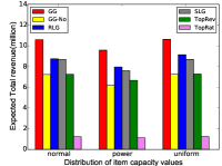 |
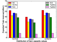 |
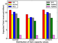 |
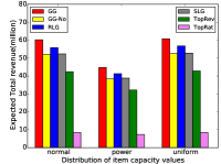 |
| (a) Amazon | (b) Epinions | (c) Amazon, class size | (d) Epinions, class size |
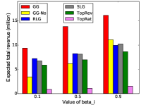 |
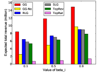 |
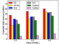 |
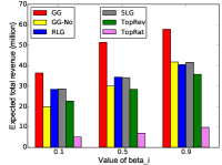 |
| (a) Amazon (Gaussian) | (b) Amazon (Exponential) | (c) Epinions (Gaussian) | (d) Epinions (Exponential) |
 |
 |
 |
 |
| (a) Amazon (Gaussian) | (b) Amazon (Exponential) | (c) Epinions (Gaussian) | (d) Epinions (Exponential) |
Synthetic Data. We use synthetic datasets much larger than Amazon and Epinions to gauge the scalability of algorithms. We do not report revenue achieved on this data, since the generation process is artificial and this dataset is solely used for testing scalability. In total there are five datasets with . is set to . The item-set is the same: and for each item , choose a value uniformly at random from , and for each time , sample uniformly at random from . For each user , we randomly choose 100 items to be the highest rated, and for each such item, sample (primitive) adoption probability values from a Gaussian distribution with and , where itself is chosen randomly from ; then we match adoption probabilities with prices so that anti-monotonicity holds. Input size will then be (cf. Table 1). Recall, the number of nonzero adoption probabilities is the critical factor in deciding the scalability of any RevMax algorithm.
Parameter Settings for Amazon and Epinions. It is unrealistic and unlikely that a user would be interested in buying all items. That is, for each user , will be nonzero for a small subset of items: we rank the items based on their predicted ratings for and compute adoption probabilities for the top-100 items. We also need the saturation factor for computing marginal revenue. We test the following two cases. First, we hard-wire a uniform value for all items, testing three different cases: , , and , representing strong, medium, and weak effect of saturation. Second, for each item , its is chosen uniformly at random from – this effectively averages over possible values for all the items to model our lack of knowledge. For capacity constraints , we consider two probability distributions from which is sampled: (1) Gaussian: for Epinions and for Amazon; (2) exponential with inverse scale (mean ). We believe the above scenarios are representative and worth testing.
Algorithms Evaluated. We compare G-Greedy, SL-Greedy, and RL-Greedy with the following natural baselines. TopRA (for Top RAting) recommends to every user the items with highest predicted rating by MF; TopRE (for Top REvenue) recommends to every user the items with highest “expected revenue” (price primitive adoption probability). Since TopRA is inherently “static”, to evaluate the expected revenue it yields over , the recommended items are repeated in all time steps. We also consider a “degenerated” version of G-Greedy, which we call GlobalNo: it ignores saturation effects when selecting triples. That is, when computing marginal revenue and selecting triples, GlobalNo will behave as though for all , but when we compute the final revenue yielded by its output strategy, the true values will be used. This is to measure how much revenue would be lost if saturation effects are present but ignored.
 |
|
|
|
| (a) Amazon | (b) Epinions | (c) Amazon, class size | (d) Epinions, class size |
 |
 |
 |
 |
 |
 |
| (a) Amazon () | (b) Amazon () | (c) Amazon () | (d) Epinions () | (e) Epinions () | (f) Epinions () |
6.2 Results and Analysis
Experimental results are reported on two metrics: expected revenue achieved (quality of recommendations, cf. Def. 2) and number of repeated recommendations made. In addition to using ground-truth information on item classes from the data, we also test the scenario with class size , i.e., each item is in its own category. For RL-Greedy, we generate permutations of . All implementations are in Java and programs were run on a Linux server with Intel Xeon CPU X5570 (2.93GHz) and 256GB RAM.
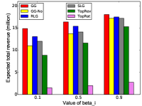
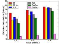
Quality of Recommendations. Figure 1 shows the expected total revenue achieved by various algorithms and baselines when is chosen uniformly at random from . As can be seen, G-Greedy consistently yields the best revenue, leading the runner-up RL-Greedy by non-trivial margins (about to gain). GlobalNo is always behind G-Greedy (about to loss), and so is SL-Greedy compared to RL-Greedy (about to behind). TopRE and TopRA are always outperformed by all greedy algorithms (though it is less so for TopRE). G-Greedy is typically to better than TopRE. Note that the expected revenues are in the scale of tens of millions dollars, so even a small relative gain could translate to large revenue.
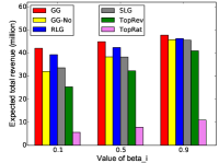
Figure 2 and Figure 3 show the comparisons of revenue with uniform values: , , and . The purpose is to examine how algorithms “react” to different strength of saturation effects. As can be seen, the hierarchy of algorithms (ranked by revenue) is quite consistent with that in Figure 1, and importantly G-Greedy is always the top performer. The gap between G-Greedy and the rest is larger with smaller (stronger saturation). In Figure 3 (class size ), though SL-Greedy is always behind RL-Greedy, the difference becomes smaller as increases. This intuitively suggests that RL-Greedy makes better decisions when it comes to repeated recommendations, as it is less sensitive to strong saturation.
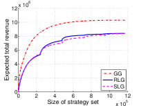
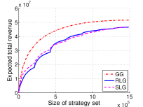
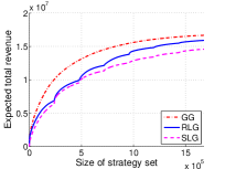
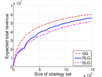
In Figure 4, we plot the growth of revenue as the greedy algorithms increment (Gaussian item quantities, uniform in ). The lines for G-Greedy clearly illustrate the phenomenon of diminishing marginal returns, empirically illustrating submodularity. Interestingly enough, SL-Greedy and RL-Greedy have similar overall trends but also have “segments”, corresponding to switches in time steps; submodularity can be observed within each “segment”.
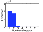
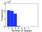
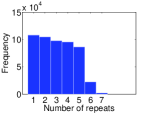
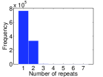
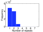
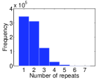
Finally, Figure 5 presents histograms on the number of repeated recommendations made by G-Greedy for each user-item pair (item class size 1; other cases are similar and hence omitted). The Y-axis is normalized to show the percentage instead of absolute counts. Note that in both datasets, when , it happens more often that an item is recommended only once or twice to a user, since the dynamic adoption probability drops rapidly with small . As becomes large, the histogram becomes less skewed as more repeats show up, especially on Amazon with . This experiment shows that G-Greedy takes advantage of (lack of) saturation for making repeat recommendations to boost revenue.
| GG | RLG | SLG | TopRE | TopRA | |
|---|---|---|---|---|---|
| Amazon | 4.67 | 6.81 | 7.95 | 0.78 | 0.45 |
| Epinions | 2.35 | 3.00 | 2.71 | 0.68 | 0.16 |
Running Time and Scalability Tests. Table 2 reports the running time of various algorithms on Amazon and Epinions. For lack of space, we only show the numbers for cases with uniform random and Gaussian item capacities (other cases are similar and hence omitted). On both datasets, G-Greedy, SL-Greedy and RL-Greedy show scalability and efficiency and all finish under 10 minutes for Amazon and under 5 minutes for Epinions.
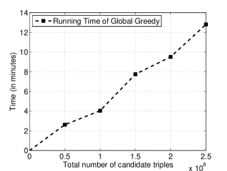
In addition, we run G-Greedy on synthetic datasets that are much larger than Amazon and Epinions. Figure 6 illustrates the running time of G-Greedy on synthetic data with 100K, 200K, 300K, 400K, and 500K users with and each user having 100 items with non-zero adoption probability. This means, for example, the dataset with 500K users has 250 million triples to select from. The growth rate in Figure 6 is almost linear and it takes about 13 minutes to finish on the largest one, which clearly demonstrates the scalability of G-Greedy. To put things in perspective, Netflix, the largest public ratings dataset, has only 100 million known ratings.
In sum, our experiments on Amazon and Epinions data show that the proposed greedy algorithms are effective and efficient, producing far superior solutions than the baselines. In particular, the most sophisticated G-Greedy consistently outperforms the rest and easily scales to (synthetic) data 2.5 times the size of the Netflix dataset.
Next, in the following subsection, we report additional experimental results conducted in the settings where information about product prices is not completely available at the beginning of a time horizon.
6.3 Experimental Results: Incomplete Product Prices
So far, our experiments have focused on the setting where all product prices, i.e., , for all in time horizon , are available as input to algorithms like G-Greedy and RL-Greedy when they are making recommendation decisions. However, this may not always be the case in practice, as prices are dynamic and exact values may not be available much in advance. Notice that this does not affect SL-Greedy as it only requires prices for the current time. As such, we are interested in gaugaing how our algorithms perform in the setting where product prices become available in batches and in time order.
 |
 |
 |
 |
| (a) Amazon (Gaussian) | (b) Amazon (power-law) | (c) Epinions (Gaussian) | (d) Epinions (power-law) |
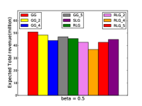
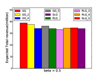
More specifically, the time horizon is “divided” into sub-horizons , and prices become available sub-horizon after sub-horizon. For example, suppose , , and . Initially, only prices for time steps through are known to the recommender system, and only at , prices for time steps through will be known. To adapt G-Greedy and RL-Greedy, the algorithms will first come up with recommendations for , and then given those, consider recommendations in . We expect both G-Greedy and RL-Greedy to yield less revenue under this setting because they are no longer able to select triples in a holistic manner for the entire horizon . Also, note that SL-Greedy is not affected at all since it already makes recommendations in chronological order.
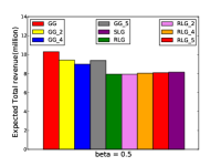
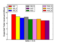
In our experiments, we set and split it into two sub-horizons, with cut-off time at , , and , respectively. For example, if cut-off is , then and . Figure 7 shows the revenue achieved by G-Greedy and RL-Greedy w.r.t. the three different cut-off time steps, and compares with the revenue yielded by these algorithms when prices are available all at once (hereafter referred to as the “original setting”). Both Amazon and Epinions datasets are used. As can be seen from Figure 7, G-Greedy (, , and ) still outperforms RL-Greedy (, , and ) and SL-Greedy. In the case of G-Greedy, , , and are all worse than the original setting (which is not surprising), and the loss is the greatest when the cut-off time is , the most even split on . This may be because when the split is not even (e.g., and ), the algorithm gets to see a larger bulk of the price information together compared with the even split (). Similar trends can be observed for RL-Greedy.
7 Extension to Random Prices
So far, we have assumed that we have access to an exact pricing model, whereby the exact price of items within a short time horizon is known. While there is evidence supporting this assumption and there are microeconomics studies on exact pricing model as pointed out in §1, the question arises what if the price prediction model is probabilistic in nature. More precisely, by treating prices as random variables, such a model only predicts them to within a distribution. Can we leverage the theory and techniques developed in this paper to deal with this case? We settle this question in this section. It is easy to see RevMax remains NP-hard, by restricting to the case where all prices are known exactly w.p. 1. The interesting question is how the algorithms can be leveraged for the random price model. In this case, the expected total revenue yielded by a strategy would be an expectation taken over the randomness of adoption events (as in the exact-pricing model) and over the randomness of prices. A major complication is that a closed form for the revenue function may not exist depending on the distribution from which prices are drawn. An obvious way of dealing with this is to treat the expected price (or most probable price) as a proxy for exact price and find a strategy that optimizes the expected revenue w.r.t. this assumption, using algorithms in §5. It is a heuristic and will clearly be suboptimal w.r.t. the true expected revenue. A more principled approach is to appeal to the Taylor approximation method used in convergence analysis [5]. It has the advantage of being distribution independent.
Consider any valid strategy , and a triple . Define . That is, contains the triples that “compete” with under . Now consider the price random variables corresponding to all triples in . E.g., if items are from the same class, , , and , then the revenue contribution of to will be dependent on the price vector . For notational simplicity, we let be this price vector for , and use to denote the -th coordinate of . In the above example, if , then . The contribution from triple to the overall revenue of is clearly a function of the price vector , and we denote it by . For all , let and be the mean and variance of respectively. Also, let be the covariance of two prices and , where . Finally, by , we mean the vector of means of the price random variables in . In our running example, , where , etc. We then expand at using Taylor’s Theorem:
| (7) |
where is the remainder (consisting of higher order terms) and by Taylor’s theorem it satisfies . Following standard practice [5], this remainder is ignored since we are interested in an efficient approximation.
Disregarding the remainder and taking expectation over both sides of (7) gives the expected revenue contribution of triple :
| (8) |
where we have applied the linearity of expectation to get . Thus, for any strategy , its expected total revenue, denoted , is .
The first three summands in (8) correspond to mean (first-order), variance, and covariance (second-order) respectively. They are used to estimate the true revenue function and the reminder is ignored. More precisely, the algorithms for the exact-price model can be used, with the calculation of revenue changed by adding the extra variance and covariance terms as shown in (8). In principle, we can incorporate as many terms from the Taylor expansion as dictated by the accuracy desired and simply use the algorithms in §5 for finding strategies with large revenue.
8 Conclusions and Future Work
In this work, we investigate the business-centric perspective of RS, and propose a dynamic revenue model by incorporating many crucial aspects such as price, competition, constraints, and saturation effects. Under this framework, we study a novel problem RevMax, which asks to find a recommendation strategy that maximizes the expected total revenue over a given time horizon. We prove that RevMax is NP-hard and develop an approximation algorithm for a slightly relaxed version (-RevMax) by establishing an elegant connection to matroid theory. We also design intelligent greedy algorithms to tackle the original RevMax and conduct extensive experiments on Amazon and Epinion data to show the effectiveness and efficiency of these algorithms. Furthermore, using synthetic data, we show that the G-Greedy algorithm scales to datasets 2.5 times the size of the Netflix dataset.
For future work, on the theoretical side, it is worth asking if RevMax remains NP-hard when every item belongs to its own class. For the random price model, it is interesting to investigate if the Taylor approximation method can yield a strategy with a guaranteed approximation to the optimal solution w.r.t. true expected revenue. In reality, it is possible that prices, saturation, and competition may interact. Modeling and learning the interactions present is an interesting challenge. On the practical side, an interesting challenge is to find suitable real datasets from which to learn the parameters for the random price model and conduct empirical evaluations on it. Finally, here we have focused on revenue-maximizing recommendation problem, given an exogenous price model. Conversely, to find optimal pricing in order to maximize the expected revenue in the context of a given RS is an interesting problem which has clear connections to algorithmic game theory [24, 28].
References
- [1] G. Adomavicius and A. Tuzhilin. Toward the next generation of recommender systems: A survey of the state-of-the-art and possible extensions. IEEE Trans. Knowl. Data Eng., 17(6):734–749, 2005.
- [2] J. Angwin and D. Mattioli. Coming soon: Toilet paper priced like airline tickets. Wall Street Journal, September 5, 2012, http://on.wsj.com/1lECovl
- [3] A. Azaria et al. Movie recommender system for profit maximization. In RecSys, pages 121–128, 2013.
- [4] Camelytics. Prices Always Change, 2012 (accessed May 9, 2014). http://bit.ly/1jznFgL.
- [5] G. Casella and R. L. Berger. Statistical Inference (2nd edition). Duxbury, 2002.
- [6] L.-S. Chen et al. Developing recommender systems with the consideration of product profitability for sellers. Inf. Sci., 178(4):1032–1048, 2008.
- [7] A. Das, C. Mathieu, and D. Ricketts. Maximizing profit using recommender systems. CoRR, abs/0908.3633, 2009.
- [8] A. Das-Sarma et al. Understanding cyclic trends in social choices. In WSDM, pages 593–602, 2012.
- [9] S. Even, A. Itai, and A. Shamir. On the complexity of timetable and multi-commodity flow problems. In FOCS, pages 184–193, 1975.
- [10] H. Gabow. An efficient reduction technique for degree-constrained subgraph and bidirected network flow problems. In STOC, pages 448–456, 1983.
- [11] H. Gabow and R. Tarjan. Faster scaling algorithms for network problems. SIAM J. Comput., 18(5):1013–1036, 1989.
- [12] Z. Gantner et al. Mymedialite: a free recommender system library. In RecSys, pages 305–308, 2011.
- [13] M. R. Garey and D. S. Johnson. Computers and Intractability: A Guide to the Theory of NP-Completeness. W. H. Freeman, 1979.
- [14] A. X. Jiang et al. Bidding agents for online auctions with hidden bids. Machine Learning, 67(1-2):117–143, 2007.
- [15] S. Kalish. A new product adoption model with price, advertising, and uncertainty. Management Science, 31(12):1569–1585, 1985.
- [16] K. Kapoor et al. Measuring spontaneous devaluations in user preferences. In KDD, pages 1061–1069, 2013.
- [17] Y. Koren. Collaborative filtering with temporal dynamics. Commun. ACM, 53(4):89–97, 2010.
- [18] Y. Koren et al. Matrix factorization techniques for recommender systems. IEEE Computer, 42(8):30–37, 2009.
- [19] J. Lee, V. S. Mirrokni, V. Nagarajan, and M. Sviridenko. Maximizing nonmonotone submodular functions under matroid or knapsack constraints. SIAM J. Discrete Math., 23(4):2053–2078, 2010.
- [20] J. Leskovec, L. A. Adamic, and B. A. Huberman. The dynamics of viral marketing. TWEB, 1(1), 2007.
- [21] F. Manshadi et al. A distributed algorithm for large-scale generalized matching. PVLDB, 6(9):613–624, 2013.
- [22] M. Minoux. Accelerated greedy algorithms for maximizing submodular set functions. In IFIP Conf. on Optimization Techniques, page 234–243, 1978.
- [23] G. D. F. Morales, A. Gionis, and M. Sozio. Social content matching in mapreduce. PVLDB, 4(7):460–469, 2011.
- [24] N. Nisan et al. Algorithmic Game Theory. Cambridge University Press, New York, NY, USA, 2007.
- [25] E. L. Porteus. Stochastic inventory theory. In Stochastic Models, volume 2, Elsevier, 1990.
- [26] F. Ricci, L. Rokach, B. Shapira, and P. B. Kantor, editors. Recommender Systems Handbook. Springer, 2011.
- [27] M. Richardson and P. Domingos. Mining knowledge-sharing sites for viral marketing. In KDD, pages 61–70, 2002.
- [28] Y. Shoham and K. Leyton-Brown. Multiagent Systems - Algorithmic, Game-Theoretic, and Logical Foundations. Cambridge University Press, 2009.
- [29] B. W. Silverman. Density estimation for statistics and data analysis, volume 26. CRC press, 1986.
- [30] C. Snyder and W. Nicholson. Microeconomic Theory, Basic Principles and Extensions (10th ed). South-Western Cengage Learning, 2008.
- [31] J. Wang and Y. Zhang. Opportunity model for e-commerce recommendation: right product; right time. In SIGIR, pages 303–312, 2013.
- [32] G. Zhao, M.-L. Lee, W. Hsu, and W. Chen. Increasing temporal diversity with purchase intervals. In SIGIR, pages 165–174, 2012.