Electrostatic Self-energy of a Charged Particle in the Surroundings of a Topologically Charged Black Hole in the Brane

Abstract

We determine the self-energy for a point charge held stationary in a topologically charged black hole spacetime arising from the Randall-Sundrum II braneworld model, showing that it has two contributions, one of geometric origin and the other of topological one.

1 Introduction

The gravitational field modifies the electrostatic interaction of a charged particle in such a way that the particle experiences a finite self-force [7, 1, 3, 5, 6, 2, 4] whose origin comes from the spacetime curvature associated with the gravitational field. However, even in the absence of curvature it was shown that a charged point particle [8, 9] or a linear charge distribution [10] placed at rest may become subject to a finite repulsive electrostatic self-force (see also [11]). In these references, the origin of the force is the distortion in the particle field caused by the lack of global flatness of the spacetime of a cosmic string. Therefore, one may conclude that the modifications of the electrostatic potential comes from two contributions: one of geometric origin and the other of topological one.

In a recent paper [12] our group studied the expression for the electrostatic potential generated by a point charge held stationary in the neighborhood of a particular solution of the Randall-Sundrum braneworld model obtained by Chamblin et. al. [13] and revisited by Sheykhi and Wang [14], which carry a topological charge arising from the bulk Weyl tensor. Here we continue this work by showing that considering this black hole as the background metric, both kinds of contributions to the self-energy, geometrical and topological, appear in the self-energy of the charged particle.

2 The Topologically Charged Black Hole in the Braneworld

The gravitational field on the brane is described by the Gauss and Codazzi equations of 5-dimensional gravity [15],

$$G_{\mu\nu}=-\Lambda g_{\mu\nu}+8\pi GT_{\mu\nu}+k_{5}^{4}\Pi_{\mu\nu}-E_{\mu\nu},$$ (1)

where $G_{\mu\nu}$ is the 4-dimensional Einstein tensor and the 5-dimensional gravity coupling constant is

$$k_{5}^{4}=\frac{48\pi G}{\tau}$$ (2)

with $\tau$ the brane tension. $T_{\mu\nu}$ is the stress-energy tensor of matter confined on the brane and $\Pi_{\mu\nu}$ is a quadratic tensor in the stress-energy tensor,

$$\Pi_{\mu\nu}=\frac{1}{12}TT_{\mu\nu}-\frac{1}{4}T_{\mu\sigma}T_{\nu}^{\>\>\sigma}+\frac{1}{8}g_{\mu\nu}\left(T_{\alpha\beta}T^{\alpha\beta}-\frac{1}{3}T^{2}\right),$$ (3)

with $T=T_{\sigma}^{\sigma}$. The tensor $E_{\mu\nu}$ is the projection of the 5-dimensional bulk Weyl tensor $C_{ABCD}$ on the brane ($E_{\mu\nu}=\delta_{\mu}^{A}\delta_{\nu}^{B}C_{ABCD}n^{A}n^{B}$ with $n^{A}$ the unit normal to the brane). Hence, $E_{\mu\nu}$ encompasses the nonlocal bulk effect and it is traceless, i.e. $E_{\sigma}^{\sigma}=0$. The 4-dimensional cosmological constant $\Lambda$ is related with the 5-dimensional cosmological constant $\Lambda_{5}$ by the relation

$$\Lambda=\frac{k_{5}^{2}}{2}\left(\Lambda_{5}+\frac{k_{5}^{2}}{6}\tau^{2}\right).$$ (4)

In this paper we will consider the Randall-Sundrum scenario in which

$$\Lambda_{5}=-\frac{k_{5}^{2}}{6}\tau^{2}$$ (5)

implying

$$\Lambda=0.$$ (6)

Under these considerations, a black hole type solution of the field equations (1) with $T_{\mu\nu}=0$ is given by the line element [16, 13, 14, 17]

$$ds^{2}=h\left(r\right)dt^{2}-\frac{dr^{2}}{h\left(r\right)}-r^{2}\left(d\theta^{2}+\sin^{2}\theta d\varphi^{2}\right)$$ (7)

where

$$h\left(r\right)=1-\frac{2GM}{r}+\frac{\beta}{r^{2}}.$$ (8)

This metric has a projected Weyl tensor, which transmits the tidal charge stresses from the bulk to the brane, with components

$$E_{\>t}^{t}=E_{\>r}^{r}=-E_{\>\theta}^{\theta}=-E_{\>\varphi}^{\varphi}=\frac{\beta}{r^{4}}.$$ (9)

Thus, the parameter $\beta$ can be interpreted as a tidal charge associated with the bulk Weyl tensor and hence, there is no restriction on it to take positive as well as negative values. If $\beta\geq 0$ there is a direct analogy to the Reissner-Nï¿œrdstrom solution because the induced metric in the domain wall presents horizons at the radii (taking $G=1$)

$$r_{\pm}=M\pm\sqrt{M^{2}-\beta}.$$ (10)

These two horizons lie inside the Schwarzschild radius $r_{s}=2M$, i.e.

$$0\leq r_{-}\leq r_{+}\leq 2M.$$ (11)

However, there is an upper limit on $\beta$, namely

$$0\leq\beta\leq\beta_{max}=M^{2}$$ (12)

which corresponds to an extremal back hole case with a degenerate horizon located at $r_{e}=M$.

As we have stated before, there is nothing to stop us choosing $\beta$ to be negative, an intriguing new possibility which leads to only one horizon,

$$r_{*}=M+\sqrt{M^{2}+\left|\beta\right|}>2M,$$ (13)

lying outside the corresponding Schwarzschild radius. In this case, the single horizon has a greater area that its Schwarzschild counterpart. Thus, one concludes that the effect of the bulk producing a negative $\beta$ is to strengthen the gravitational field outside the black hole (obviously it also increase the entropy and decrease the Hawking temperature). We will show that a negative value of $\beta$ also produces a decrease in the electrostatic self-energy of a charged particle located outside the horizon.

Performing the change of the radial coordinate

$$r=\rho+M+\frac{M^{2}-\beta}{4\rho},$$ (14)

gives the line element (7) in the isotropic coordinate system $\left(t,\rho,\theta,\varphi\right)$

$$ds^{2}=N^{2}\left(\rho\right)dt^{2}-B^{2}\left(\rho\right)\left(d\rho^{2}+\rho^{2}d\Omega^{2}\right)$$ (15)

where $N^{2}\left(\rho\right)=\frac{1}{r^{2}}\left[\rho-\frac{M^{2}-\beta}{4\rho}\right]^{2}$and $B^{2}\left(\rho\right)=\frac{r^{2}}{\rho^{2}}$. Using these coordinates, the horizons are located at the values $\rho_{\pm}$ defined by the relation

$$N\left(\rho_{\pm}\right)=0$$ (16)

and the surface gravity at the horizon is

$$\kappa=\frac{1}{B\left(\rho_{+}\right)}\left.\frac{dN}{d\rho}\right|_{\rho=\rho_{+}}.$$ (17)

From this expression and assuming that $\kappa B\left(\rho_{+}\right)\neq 0$, we can write

$$N\left(\rho\right)\propto\kappa B\left(\rho_{+}\right)\left(\rho-\rho_{+}\right)\mbox{ when }\rho\rightarrow\rho_{+}.$$ (18)

Similar relations for the $\beta<0$ case are obtained by replacing $r_{+}$ with $r_{*}$ ( or $\rho_{+}$ with $\rho_{*}$ correspondingly).

3 The Electrostatic Field of a Point Particle

Copson [18] and Linet [19] found the electrostatic potential in a closed form of a point charge at rest outside the horizon of a Schwarzschild black hole and that the multipole expansion of this potential coincides with the one given by Cohen and Wald [20] and by Hanni and Ruffini [21]. In this section we will investigate this problem in the background of the topologically charged black hole (7). If the electromagnetic field of the point particle is assumed to be sufficiently weak so its gravitational effect is negligible, the Einstein-Maxwell equations reduce to Maxwell’s equations in the curved background (15). In the electrostatic case, the spatial components of the potential vanish, $A^{i}=0$, while the temporal component $A^{0}=\phi$ is determined by the equation

$$\frac{1}{\sqrt{g}}\partial_{i}\left(\sqrt{g}g^{00}g^{ij}\partial_{j}A_{0}\right)=4\pi J^{0}$$ (19)

where $J^{0}$ is the charge density. When considering a point test charge $q$ held stationary at $\left(\rho_{0},\theta_{0},\varphi_{0}\right)$, with $\rho_{0}>\rho_{+}$ in the case $\beta\geq 0$ or $\rho_{0}>\rho_{*}$ in the case $\beta<0$, the associated current density $J^{i}$ vanishes while the charge density $J^{0}$ is given by

$$J^{0}=\frac{q}{\sqrt{g}}\delta\left(\rho-\rho_{0}\right)\delta\left(\theta-\theta_{0}\right)\delta\left(\varphi-\varphi_{0}\right).$$ (20)

Choosing, without loss of generality, $\theta_{0}=0$, equation (19) becomes

$$\nabla^{2}A_{0}+\frac{N}{B}\frac{\partial}{\partial\rho}\left(\frac{B}{N}\right)\partial_{\rho}A_{0}=-4\pi\frac{q}{\rho^{2}}\frac{N}{B}\delta\left(\rho-\rho_{0}\right)\delta\left(\cos\theta-1\right)$$ (21)

where $\nabla^{2}$ is the Laplacian operator. The behavior of $A_{0}$ in the neighbourhood of the point $\left(\rho=\rho_{0},\theta=0\right)$ is given by

$$A_{0}\left(\rho,\theta\right)\sim\frac{N\left(\rho_{0}\right)}{B\left(\rho_{0}\right)}\frac{q}{\sqrt{\rho^{2}-2\rho\rho_{0}\cos\theta+\rho_{0}^{2}}}.$$ (22)

In order to obtain the solution of this equation near the horizon and in the far region, we expand $A_{0}$ in spherical harmonics,

$$A_{0}\left(\rho,\theta\right)=\sum_{l=0}^{\infty}R_{l}\left(\rho,\rho_{0}\right)P_{l}\left(\cos\theta\right)$$ (23)

where the radial function satisfies the differential equation

$$\frac{d^{2}R_{l}}{d\rho^{2}}+\left(\frac{2}{\rho}+\frac{1}{B}\frac{dB}{d\rho}-\frac{1}{N}\frac{dN}{d\rho}\right)\frac{dR_{l}}{d\rho}-\frac{l\left(l+1\right)}{\rho^{2}}R_{l}=-q\left(2l+1\right)\frac{N}{B}\frac{\delta\left(\rho-\rho_{0}\right)}{\rho^{2}}.$$ (24)

Now we need to define two linearly independent solutions $g_{l}$ and $f_{l}$ with the appropriate boundary solutions, so we will impose that the electric field derived from the obtained electrostatic potential should be well behaved at the horizon and at the spatial infinity of the black hole. For $l=0$, equation (24) can be integrated to obtain the condition

$$\frac{dR_{0}\left(\rho\right)}{d\rho}\propto\frac{1}{\rho^{2}}\frac{N\left(\rho\right)}{B\left(\rho\right)}.$$ (25)

Thus, we consider the functions

$$g_{0}\left(\rho\right)=1$$ (26)

and

$$f_{0}\left(\rho\right)=a\left(\rho\right)=\int_{\rho}^{\infty}\frac{N\left(\rho^{\prime}\right)}{\rho^{\prime 2}B\left(\rho^{\prime}\right)}d\rho^{\prime}.$$ (27)

Function $a\left(\rho\right)$ is finite at the horizon and its value will be denoted $a_{+}=a\left(\rho_{+}\right)$. For $l\neq 0$ equation (24) has a singular point of regular type at $r=r_{+}$ because from eq. (18) we have

$$\frac{1}{N}\frac{dN}{d\rho}\propto\frac{1}{\rho-\rho_{+}}\mbox{ when }\rho\rightarrow\rho_{+}.$$ (28)

The roots of the indicial equation relative to this point are $0$ and $2$ and therefore we have a regular solution at the horizon that we will denote

$$g_{l}\left(\rho\right)\propto\left(\rho-\rho_{+}\right)^{2}\mbox{ when }\rho\rightarrow\rho_{+},$$ (29)

and that gives a well behaved electric field at the horizon but is singular at $\rho\rightarrow\infty$. This fact shows that the black hole does not have multipole electric moments, except for the monopole. On the other hand, the regular solution at $\rho\rightarrow\infty$ will be denoted $f_{l}\left(\rho\right)$ and following a similar argument, it will be singular at the horizon. In conclusion, the electrostatic potential with the adequate boundary conditions is written

$$A_{0}\left(\rho,\theta\right)=\begin{cases}qa\left(\rho_{0}\right)+q\sum_{l=1}^{\infty}C_{l}g_{l}\left(\rho\right)f_{l}\left(\rho_{0}\right)P_{l}\left(\cos\theta\right)&\mbox{ for }\rho_{+}<\rho<\rho_{0}\\ qa\left(\rho\right)+q\sum_{l=1}^{\infty}C_{l}g_{l}\left(\rho_{0}\right)f_{l}\left(\rho\right)P_{l}\left(\cos\theta\right)&\mbox{ for }\rho>\rho_{0}\end{cases}$$ (30)

where the constant coefficients $C_{l}$ are determined by equation (24).

4 Electrostatic Self-Energy

As is well known, the Coulombian part of the electrostatic potential $A_{0}$ does not yield an electrostatic self-force associated with the Killing vector $\partial_{0}$. However, the regular part of the potential at $\rho=\rho_{0}$ and $\theta=0$ defines an electrostatic self-energy $W_{self}\left(\rho_{0}\right)$. As noted in [6, 4, 2], this energy can be obtained through the limit

$$\frac{q}{2}\left[A_{0}\left(\rho,\theta\right)-\frac{N\left(\rho_{0}\right)}{B\left(\rho_{0}\right)}\frac{q}{\sqrt{\rho^{2}-2\rho\rho_{0}\cos\theta+\rho_{0}^{2}}}\right]\rightarrow W_{self}\left(\rho_{0}\right)\mbox{ when $\rho\rightarrow\rho_{0}$ and $\theta\rightarrow$0. }$$ (31)

From this expression it is clear that the Coulombian part of the electrostatic potential, represented by equation (22) does not yield an electrostatic self-force. Therefore, in order to calculate the self-energy we will use the result of our previous work [12] where we have shown that the electrostatic potential of a charged particle in the background of a topological charged black hole (7) satisfies the differential equation (19) in isotropic coordinates with the coefficient

$$\frac{N\left(\rho\right)}{B\left(\rho\right)}=\frac{\left(1-\frac{\sqrt{M^{2}-\beta}}{2\rho}\right)}{\left(1+\frac{\sqrt{M^{2}-\beta}}{2\rho}\right)^{3}}.$$ (32)

The solution of the electrostatic solution in isotropic coordinates, obtained by using the Hadamard method [18] and denoted as $\phi_{C}$, has the same behavior as equation (22) in the neighborhood of the point $\left(\rho=\rho_{0},\theta=0\right)$,

$$\tilde{\phi}\left(\rho,\theta\right)\sim\frac{\left(1-\frac{\sqrt{M^{2}-\beta}}{2\rho_{0}}\right)}{\left(1+\frac{\sqrt{M^{2}-\beta}}{2\rho_{0}}\right)^{3}}\frac{q}{\sqrt{\rho^{2}-2\rho\rho_{0}\cos\theta+\rho_{0}^{2}}}.$$ (33)

Replacing this condition in equation (31) we obtain the limit process

$$\frac{q}{2}\left[A_{0}\left(\rho,\theta\right)-\frac{N\left(\rho_{0}\right)}{B\left(\rho_{0}\right)}\frac{\left(1+\frac{\sqrt{M^{2}-\beta}}{2\rho_{0}}\right)^{3}}{\left(1-\frac{\sqrt{M^{2}-\beta}}{2\rho_{0}}\right)}\tilde{\phi}\left(\rho,\theta\right)\right]\rightarrow W_{self}\left(\rho_{0}\right)$$ (34)

as $\rho\rightarrow\rho_{0}$ and $\theta\rightarrow 0$. Using Gauss’ theorem it has been shown [12] that $\tilde{\phi}$ describes a secondary charge with value $-\frac{q\sqrt{M^{2}-\beta}}{\rho_{0}\left(1+\frac{\sqrt{M^{2}-\beta}}{2\rho_{0}}\right)^{2}}$ inside the horizon. Hence, the multipole expansion of the potential $\phi_{C}$ gives

$$\tilde{\phi}\left(\rho,\theta\right)=\begin{cases}\frac{q}{\rho_{0}\left(1+\frac{\sqrt{M^{2}-\beta}}{2\rho_{0}}\right)^{2}}\left[1-\frac{\sqrt{M^{2}-\beta}}{\rho\left(1+\frac{m}{2\rho}\right)^{2}}\right]+q\sum_{l=1}^{\infty}\tilde{C}_{l}\tilde{g}_{l}\left(\rho\right)\tilde{f}_{l}\left(\rho_{0}\right)P_{l}\left(\cos\theta\right)&\mbox{ for }\rho_{+}<\rho<\rho_{0}\\ \frac{q}{\rho\left(1+\frac{\sqrt{M^{2}-\beta}}{2\rho}\right)^{2}}\left[1-\frac{\sqrt{M^{2}-\beta}}{\rho_{0}\left(1+\frac{\sqrt{M^{2}-\beta}}{2\rho_{0}}\right)^{2}}\right]+q\sum_{l=1}^{\infty}\tilde{C}_{l}\tilde{g}_{l}\left(\rho_{0}\right)\tilde{f}_{l}\left(\rho\right)P_{l}\left(\cos\theta\right)&\mbox{ for }\rho>\rho_{0}.\end{cases}$$ (35)

Replacing the multipole expansions (30) and (35) in equation (34) and setting $\rho=\rho_{0}$ and $\theta=0$ in the infinite series it is possible to evaluate $W_{self}\left(\rho_{0}\right)$. However, we are interested in the determination of the electrostatic self-energy on the horizon, so we also take the limit $\rho_{0}\rightarrow\rho_{+}$. Each term in the infinite series labeled by $l=1,2,3,...$ contains the polynomials $g_{l}\left(\rho_{+}\right)$ or $\tilde{g}_{l}\left(\rho_{+}\right)$ which vanish because of property (29). Hence, only the monopole terms in the multipole expansions contribute to the limit process, giving the final result as

$$W_{self}=\frac{q^{2}}{2}\left(a_{+}-\kappa\right)$$ (36)

with $a_{+}$ defined in equation (27) and the surface gravity $\kappa$ appearing in the limit process through

$$\kappa=\lim_{\rho_{0}\rightarrow\rho_{+}}\frac{N\left(\rho_{0}\right)}{\rho_{+}B\left(\rho_{+}\right)\left(1-\frac{\sqrt{M^{2}-\beta}}{2\rho_{0}}\right)}$$ (37)

where we used equation (18). Obviously, the self-energy given in (36) is independent of the choice of the radial coordinate. In terms of the radial coordinate $r$ in which the line element of the topologically charged black hole is given by equation (7), it is straightforward to calculate

$$a_{+}=\int_{r_{+}}^{\infty}\frac{dr}{r^{2}}=\frac{1}{r_{+}}$$ (38)

and

$$\kappa=\frac{\sqrt{M^{2}-\beta}}{r_{+}^{2}},$$ (39)

and therefore the self-energy is simply

$$W_{self}=\frac{q^{2}}{2}\frac{M}{r_{+}^{2}}.$$ (40)

A similar analysis can be performed in order to consider the $\beta<0$ black hole case, obtaining the final result

$$W_{self}=\frac{q^{2}}{2}\frac{M}{r_{*}^{2}}$$ (41)

where the horizon radius $r_{*}$ is given by equation (13).

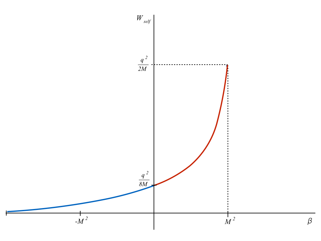
Figure 1: Self-energy of a particle with electric charge $q$ in the background of the topologically charged black hole as function of the topological charge $\beta$. The red section gives the behavior for $0<\beta<M^{2}$ while the blue section shows the self-energy when $\beta<0$.

Figure 1 shows the complete behavior of the self-energy of the particle with electric charge $q$ in the background of the topologically charged black hole. The red section gives the behavior for a topological charge in the range $0<\beta<M^{2}$ while the blue section shows the self-energy when $\beta<0$. Note that the extremal black hole, characterized by the condition $\beta=M^{2}$, gives a self-energy $W_{self}=\frac{q^{2}}{2M}$ which is the same value obtained for the extreme Reissner-Nordstrï¿œm black hole [23, 22], due to the similarities between both metrics. Similarly, the self-energy for the Schwarschild metric corresponds to the point $\beta=0$ giving $W_{self}=\frac{q^{2}}{8M}$ [6, 2, 4]. Finally, it is interesting to note that the self-energy of the particle goes to zero as the bulk geometry is such that $\beta\rightarrow-\infty$, a behavior that never appears in the Reissner-Nordstrï¿œm case. This fact shows that the complete curve in Figure 1 represents a self-energy which has two kinds of contributions, one of geometric origin (through the mass of the black hole) and the other of topological one (appearing in our analysis through the bulk Weyl tensor).

This work was supported by the Universidad Nacional de Colombia. Hermes Project Code 18140.

References

- [1] B. Ĺeaut́e and B. Linet, Class. Quantum Grav. 1, 5 (1985)
- [2] B. Ĺeaut́e and B. Linet, Int. J. Theor. Phys. 22, 67 (1983)
- [3] F. Piazzese and G. Rizzi, Phys. Lett. A 119, 7 (1986)
- [4] A. I. Zel’nikov and V. P. Frolov, Sov. Phys. JETP 55, 191(1982)
- [5] B. Boisseau, C. Charmousis and B. Linet, Class. Quantum Grav. 13, 1797 (1996)
- [6] A. G. Smith and Clifford M. Will, Phys Rev. D 22, 1276 (1980)
- [7] A. Vilenkin, Phys Rev. D 20, 373 (1979)
- [8] B. Linet, Phys. Rev. D 33, 1833 (1986)
- [9] A. G. Smith, Proceedings of the Symposium The Formation and Evolution of Cosmic Strings, ed. G. W. Gibbons, S. W/. Hawking and T. Vaschapati (Cambridge University Press, Cambridge, 1990), p.262.
- [10] E. R. Bezerra de Mello, V. B. Bezerra, C. Furtado and F. Moraes, Phys. Rev. D 51, 7140 (1995)
- [11] J. Spinelly and V. B. Bezerra. Mod. Phys. Lett. A 15, 1961-1966 (2000)
- [12] A. Larranaga, N. Herrera, and S. Ramirez, “Electrostatics in the Surroundings of a Topologically Charged Black Hole in the Brane,” Advances in High Energy Physics, vol. 2014, Article ID 146094, 6 pages, 2014. doi:10.1155/2014/146094
- [13] A. Chamblin, H.S. Reall, H. Shinkai and T. Shiromizu, Phys. Rev. D 63, 064015 (2001)
- [14] A. Sheykhi and B. Wang. Mod. Phys. Lett. A 24, 2531-2538 (2009)
- [15] T. Shiromizu, K. Maeda and M. Sasaki, Phys. Rev. D 62, 024012 (2000)
- [16] N. Dadhich, R. Maartens, P. Papadopoulos and V. Rezania, Phys. Lett. B 487, 1 (2000)
- [17] C. G. Bï¿œmer, T. Harko and F. S. N. Lobo. Class. Quantum Grav. 25, 045015 (2008)
- [18] E. Copson. Proc. R. Soc. A 118, 184-194 (1928)
- [19] B. Linet, J. Phys. A 9, 1081 (1976)
- [20] J, Cohen and R. Wald. J. Math. Phys. 12, 1845-1849 (1971)
- [21] R. Hanni and R. Ruffini. Phys. Rev. D 8 3259-3265 (1973)
- [22] B. Ĺeaut́e and B. Linet, Phys. Lett. A 58, 1. 5-6 (1976)
- [23] B. Linet. Phys. Rev. D 61, 107502 (2000)