Diffusion-Based Coarse Graining in Hybrid Continuum–Discrete Solvers: Applications in CFD–DEM

Abstract

In this work, a coarse-graining method previously proposed by the authors in a companion paper based on solving diffusion equations is applied to CFD–DEM simulations, where coarse graining is used to obtain solid volume fraction, particle phase velocity, and fluid–particle interaction forces. By examining the conservation requirements, the variables to solve diffusion equations for in CFD–DEM simulations are identified. The algorithm is then implemented into a CFD–DEM solver based on OpenFOAM and LAMMPS, the former being a general-purpose, three-dimensional CFD solver based on unstructured meshes. Numerical simulations are performed for a fluidized bed by using the CFD–DEM solver with the diffusion-based coarse-graining algorithm. Converged results are obtained on successively refined meshes, even for meshes with cell sizes comparable to or smaller than the particle diameter. This is a critical advantage of the proposed method over many existing coarse-graining methods, and would be particularly valuable when small cells are required in part of the CFD mesh to resolve certain flow features such as boundary layers in wall bounded flows and shear layers in jets and wakes. Moreover, we demonstrate that the overhead computational costs incurred by the proposed coarse-graining procedure are a small portion of the total computational costs in typical CFD–DEM simulations as long as the number of particles per cell is reasonably large, although admittedly the computational overhead of the coarse-graining procedure often exceeds that of the CFD solver. Other advantages of the diffusion-based algorithm include more robust and physically realistic results, flexibility and easy implementation in almost any CFD solvers, and clear physical interpretation of the computational parameter needed in the algorithm. In summary, the diffusion-based method is a theoretically elegant and practically viable option for practical CFD–DEM simulations.

1 Introduction

1.1 Particle-Laden Flows: Physical Background and Multi-Scale Modeling

Particle-laden flows occur in many settings in natural science and engineering, e.g., sediment transport in rivers and coastal oceans, debris flows during flooding, cuttings transport in petroleum-well drilling, as well as powder handling and pneumatic conveying in pharmaceutical industries (Sifferman et al., 1974; Nielsen, 1992; Iverson, 1997; Yang, 1998). In particular, this work is concerned with the dense-phase regime, where both the fluid–particle interactions and the inter-particle collisions play important roles. For examples, the dense particle-laden flows in fluidized beds in chemical reactors and the sheet flows in coastal sediment transport both fall within this regime.

Various numerical simulation approaches have been proposed for particle-laden flows in the past few decades. Among the most established and most commonly used is the Two-Fluid Model (TFM) approach, which describes both the fluid phase and the particle phase as inter-penetrating continua (Sun et al., 2007). The two sets of mass and momentum conservation equations for the two phases are solved with mesh-based numerical discretization, with coupling terms accounting for the interaction forces between the phases. Particles are not explicitly resolved or represented in the TFM formulation, although the particle phase properties do take into account certain particle characteristics. Therefore, the computational cost of the two-fluid model is relatively low, and thus this method is widely used in industrial applications, where fast turnover times are often a critical requirement. However, the physics of the particle or granular flows are fundamentally different from that of fluids. Among many other difficulties associated with the TFM, a critical issue with this approach is that a universal constitutive relation for the particle phase that is applicable to different flow regimes seems to be lacking despite much research on this topic (Sun and Sundaresan, 2011). This difficulty stems from the fact that unlike the flow of real continuum fluids (gases or liquids) where strong separation of scales justifies the continuum description, in granular flows the scale separation is weak (Glasser and Goldhirsch, 2001), i.e., the representative volume element can be of a similar order of magnitude to particle diameters. As such, a continuum description of the particle phase would suffer from these intrinsic difficulties. Other drawbacks of the TFM approach include the difficulty in representing particles with a continuous distribution of diameters or densities and the reliance on empirical models of fluid–particle interactions, among others (Sun et al., 2009).

On the other hand, direct numerical simulations based on Lattice-Boltzmann method (Yin and Koch, 2008) or by solving Navier–Stokes equations with fluid–particle interfaces fully resolved (e.g., via immersed boundary method (Kempe et al., 2014)) are computationally expensive. The DNS methods are currently limited to systems of $O(10^{3})$ particles in spite of sustained rapid growth of available computational resources in the past decades. Interestingly, this difficulty is also due to the fact that multiple scales do exist in the particle-laden flow problem, although the scale separation is weak, as explained above. That is, the scales of concern are several orders of magnitude larger than the particle diameter $d_{p}$, and thus the simulated system may contain a large number of particles. It is expected that DNS will not be affordable for simulating realistic dense particle-laden flows in the near future, where the number of particles can be $O(10^{6})$ or even more.

In view of the multi-scale nature of and the weak scale-separation in dense particle-laden flows, the continuum–discrete approach seems to be a natural choice. In this approach, continuum model is used to describe the fluid phase, while the particle phase is described by the Discrete Element Method (DEM) , where particles are tracked individually based on Newton’s second law in a Lagrangian framework. DEM was first used to model granular flow without interstitial fluids in geotechnical engineering in the 1970s (Cundall and Strack, 1979). The hybrid CFD–DEM approach to model particle-laden flows was attempted in the 1990s (Tsuji et al., 1993). Traditionally the locally averaged Navier–Stokes equations are adopted as the continuum model (Anderson and Jackson, 1967), leading to a hybrid method commonly referred to as CFD–DEM (Computational Fluid Dynamics–Discrete Element Method). Recently, Large Eddy Simulation (LES), a CFD technology based on the solution of filtered Navier–Stokes equations, has been used as the continuum fluid model, leading to hybrid LES–DEM solvers (Zhou et al., 2004). Other variations in the category of continuum–discrete solvers include those using Smooth Particle Hydrodynamics (SPH) or Lattice-Boltzmann for the fluid flow (Han et al., 2007; Sun et al., 2013).

1.2 Coarse Graining in Continuum–Discrete Particle-Laden Flow Solvers

In all these continuum–discrete particle-laden flow solvers mentioned above including CFD–DEM and LES–DEM, one needs to bridge the continuum-based conservation equations for the fluid phase and the discrete description of the particle phase. Specifically, the presence and the dynamic effects of the particles on the fluid are taken into account in the fluid continuity and momentum equations through the macroscopic quantities of the particle phase, e.g., solid volume fraction $\varepsilon_{s}$, solid phase velocity $\mathbf{U}_{s}$, and solid–fluid interphase forces $\mathbf{F}^{fp}$. These Eulerian field quantities are not solved for in the continuum-scale solver, but need to be obtained from the discrete particle information (i.e., individual particle locations $\mathbf{x}$, particle velocities $\mathbf{u}$, interaction forces on individual particles $\mathbf{f}^{fp}$). The process of obtaining macroscopic quantities from particle-scale quantities is referred to as coarse graining in this work.

In CFD–DEM or LES–DEM solvers the fluid equations are discretized with mesh-based numerical methods such as finite volume for finite element methods. From here on we focus our discussions on CFD–DEM for brevity. However, note that the discussions presented and the methods proposed in this work shall be equally applicable to LES–DEM solvers, and may be useful for other continuum–discrete methods such as SPH–DEM and LB-DEM for particle-laden flows. Another method that is closely related to CFD/LES–DEM is the Particle-in-Cell (PIC) method, which is widely used in plasma simulations (Dawson, 1983), where individual physical particles (electrons, ions, etc.) or “super-particles” that represent a number of physical particles of similar properties are tracked in a Lagrangian framework. The interactions among the particles are computed not in a pair-wise way but via electric and magnetic fields that are Eulerian field quantities computed from the particle distribution data. The coarse graining is an important ingredient in the PIC method, and the proposed method can be of relevance there.

Details on how the solid phase quantities interact with the fluid phase quantities in CFD–DEM will be presented in Section 2 after the mathematical formulation for the method is introduced. In CFD–DEM solvers the Eulerian field quantities of the fluid phase become cell-based quantities after numerical discretization. Therefore, to bridge continuum-based description of the fluid phase and the discrete description of the particle phase, we simply need to obtain cell-based representation of the Eulerian field quantities (e.g., solid volume fraction $\varepsilon_{s}$, Eulerian velocity $\mathbf{U}_{s}$, and fluid–particle interaction forces $\mathbf{F}^{fp}$) of the solid phase. A straightforward and probably the most widely used method to link particle quantities and cell quantities is the Particle Centroid Method (PCM). The PCM utilizes the fluid mesh for coarse graining by summing over all particle volumes in each cell to obtain cell-based solid volume fraction $\varepsilon_{s}$, and similar procedures are followed for other variables such as $\mathbf{U}_{s}$ and $\mathbf{F}^{fp}$. This method is very straightforward to implement in almost any CFD solvers, but it can lead to large errors when cell size to particle diameter ratios are small. Consequently, various alternatives have been proposed to improve the accuracy of PCM. The Divided Particle Volume Method (DPVM), first proposed and implemented by Wu et al. (2009a, b), is such an example. In this method, the volume of a particle is divided among all cells that it overlaps with according to the portion of the volume within each cell, and is not only distributed entirely to the cell its centroid resides in as in PCM. As a consequence, the DPVM at least guarantees that the solid volume fraction $\varepsilon_{s}$ in any cell should never exceed one, effectively preventing very large gradients in the obtained $\varepsilon_{s}$ field. DPVM works for arbitrary meshes, structured or unstructured, with any elements shapes as long as any edge of the cell has a length larger than the particle diameter. Comprehensive comparisons between DPVM and PCM recently performed by Peng et al. (2014) suggest that DPVM has significantly improved performance over PCM. Another idea, recently proposed by Deb and Tafti (2013), is to use two separate meshes for the CFD discretization and the coarse graining. While the improved variants do outperform the PCM in terms of accuracy, the implementations of these sophisticated methods are often significantly more complicated, especially in CFD solver based on unstructured, non-Cartesian meshes.

In our efforts to develop a CFD/LES–DEM solver with a parallel, three dimensional CFD code based on unstructured meshes with arbitrary cells shapes, we found that none of existing coarse-graining methods is able to satisfy the requirements of easy implementation and good accuracy simultaneously. The difficulties motivated us to develop a coarse-graining method that is suitable for practical implementation in general-purpose CFD/LES–DEM solvers, while maintaining the theoretical rigor and excellent accuracy.

The general motivation, description, and derivation of the diffusion-based coarse-graining method as well as a priori tests (where no CFD–DEM simulations were performed) have been presented in Sun and Xiao (2014). Specifically, the companion paper (1) comprehensively reviewed and compared existing coarse-graining methods in the literature, including PCM, DPVM, two-grid formulation, and statistical kernel methods, (2) motivated and proposed a diffusion-based coarse-graining method, (3) demonstrated the equivalence (up to the mesh discretization accuracy) between the current method and the statistical kernel-based coarse-graining method with Gaussian kernel, and (4) evaluated the performance of the diffusion-based method by comparing it with existing methods in various scenarios, with both structured and unstructured meshes, and both in the interior domain and near wall boundaries. While maintaining all the merits of its theoretically equivalent counterpart such as mesh-independence, the diffusion-based method is much easier for practical implementations in general-purpose CFD–DEM solvers, and provides a unified framework for treating interior particles and particles that are located near boundaries.

The present work is a companion paper of Sun and Xiao (2014). The objective is to explore the theoretical and practical issues of applying the diffusion-based coarse-graining method in a general-purpose CFD–DEM solver, and to evaluate its performance in practical fluidized bed simulations. Specifically, in this paper (1) the conservation characteristics of the diffusion-based coarse-graining method are studied, based on which the variables to solve diffusion equations for are identified (i.e., $\varepsilon_{s}$, $\varepsilon_{s}\mathbf{U}_{s}$, $\varepsilon_{f}\mathbf{F}^{fp}$), (2) the algorithm is implemented into a CFD–DEM solver and tested in fluidized bed simulations, highlighting the improved mesh-convergence behavior compared to the PCM, and (3) the choice of diffusion bandwidth is justified based on physical reasoning. The issues discussed in the present work (e.g, the in-situ performance of the proposed coarse-graining method in CFD–DEM solvers, as well as the choice of variables to solve diffusion equations for and the diffusion bandwidth) are specific to the application of the diffusion-based method in CFD–DEM simulations. These issues are not trivial and warrant thorough investigations.

The rest of the paper is organized as follows. Section 2 introduces the mathematical formulation of the CFD–DEM approach, gives a summary of the diffusion-based coarse-graining method, and then discusses their numerical implementations and the numerical methods used in the simulations. In Section 3 CFD–DEM simulations are conducted by using the proposed coarse-graining method, and the results are discussed and compared with those obtained with PCM. The overhead computational costs associated with the coarse-graining procedure are investigated in a series of cases with different ratios of particle and cell numbers. The physical basis of choosing the bandwidth parameter in the diffusion-based method and possible extensions to spatial–temporal averaging are discussed in Section 4. Finally, Section 5 concludes the paper.

2 Methodology

2.1 Mathematical Formulations of CFD–DEM

Due to the large number of symbols and subscripts used in this paper, it is beneficial to establish certain conventions in the notations before proceeding to the presentation of the particle and fluid phase equations. Unless noted otherwise, superscripts are used to categorize the physical background associated with a quantity, e.g., ‘$col$’ for collision, ‘$fp$’ for fluid–particle interactions, etc. These superscripts should be relatively self-evident. Phase subscripts are used to denote quantities associated with solid phase (‘$s$’), fluid phase (‘$f$’), individual particles (‘$p$’), and individual cells (‘$c$’). Index subscripts $i$ and $k$ are used as indices for particles and cells, respectively. To avoid further cluttering of indices, vector notations are preferred to tensor notations throughout the paper. When a quantity has both the indices ($i$ or $k$) and phase subscripts ($s$, $f$, $p$, or $c$), they are separated by a comma. The particle-level velocities and the forces associated with individual particles are denoted as $\mathbf{u}$ and $\mathbf{f}$, respectively; and the velocities and forces in the continuum scale are denoted as $\mathbf{U}$ and $\mathbf{F}$, respectively.

2.1.1 Discrete Element Method for Particles

In the CFD–DEM approach, the translational and rotational motion of each particle is described by the following equations (Cundall and Strack, 1979; Ball and Melrose, 1997; Weber et al., 2004):

$$m\frac{d\mathbf{u}}{dt} =\mathbf{f}^{col}+\mathbf{f}^{fp}+m\mathbf{g}$$ (1a)

$$I\frac{d\boldsymbol{\Psi}}{dt} =\mathbf{T}^{col}+\mathbf{T}^{fp}$$ (1b)

where $\mathbf{u}$ is the particle velocity; $t$ is time; $m$ is particle mass; $\mathbf{f}^{col}$ is the force due to collisions and enduring contacts with other particles or wall boundaries; $\mathbf{f}^{fp}$ denotes the forces due to fluid–particle interactions, e.g., drag, lift, and buoyancy; $\mathbf{g}$ denotes external body forces. Similarly, $I$ and $\mathbf{\Psi}$ are angular moment of inertia and angular velocity, respectively, of the particle; $\mathbf{T}^{col}$ and $\mathbf{T}^{fp}$ are the torques due to particle–particle interactions and fluid–particle interactions, respectively. For the purpose of computing collision forces and torques, the particles are modeled as soft spheres with interparticle contact represented by an elastic spring and a viscous dashpot. Further details can be found in the literature (e.g., Cundall and Strack, 1979; Tsuji et al., 1993; Xiao and Sun, 2011).

2.1.2 Locally-Averaged Navier–Stokes Equations for Fluids

The fluid phase is described by the locally averaged incompressible Navier–Stokes equations. Assuming constant fluid density $\rho_{f}$, the continuity and momentum equations for the fluid are (Anderson and Jackson, 1967; Kafui et al., 2002):

$$\nabla\cdot\left(\varepsilon_{s}\mathbf{U}_{s}+{\varepsilon_{f}\mathbf{U}_{f}}\right) =0,$$ (2a)

$$\frac{\partial\left(\varepsilon_{f}\mathbf{U}_{f}\right)}{\partial t}+\nabla\cdot\left(\varepsilon_{f}\mathbf{U}_{f}\mathbf{U}_{f}\right) =\frac{1}{\rho_{f}}\left(-\nabla p+\nabla\cdot{\boldsymbol{\mathcal{R}}}+\varepsilon_{f}\rho_{f}\mathbf{g}+\mathbf{F}^{fp}\right),$$ (2b)

where $\varepsilon_{s}$ is the solid volume fraction; $\varepsilon_{f}=1-\varepsilon_{s}$ is the fluid volume fraction; $\mathbf{U}_{f}$ is the fluid velocity. The four terms on the right hand side of the momentum equation are pressure ($p$) gradient, divergence of stress tensor $\boldsymbol{\mathcal{R}}$ (including viscous and Reynolds stresses), gravity, and fluid–particle interactions forces, respectively. Since the equations are formulated in the Eulerian framework, all variables herein are continuum quantities, i.e., they are mesh-based when discretized numerically. As explained in Section 1.1, the solid phase quantities $\varepsilon_{s}$, $\mathbf{U}_{s}$, $\mathbf{F}^{fp}$ are not explicitly solved for, but are instead obtained from the particle information via coarse-graining procedures.

2.1.3 Fluid–Particle Interactions

While the fluid–particle interaction force $\mathbf{F}^{fp}$ consists of many components including buoyancy $\mathbf{F}^{buoy}$, drag $\mathbf{F}^{drag}$, force, and Basset history force, among others, here we focus on the drag term for the purpose of illustrating the bridging between the continuum and discrete scales. Other forces can be coarse grained in a similar way. In PCM-based coarse graining, the particle drag on the fluid is obtained by summing the drag over all particle in a cell. The drag on an individual particle $i$ is generally formulated as:

$$\mathbf{f}^{drag}_{i}=\frac{V_{p,i}}{\varepsilon_{f,i}\varepsilon_{s,i}}\beta_{i}\left(\mathbf{u}_{p,i}-\mathbf{U}_{f,i}\right),$$ (3)

where $V_{p,i}$, and $\mathbf{u}_{p,i}$ are the volume, and the velocity, respectively, of particle $i$; $\mathbf{U}_{f,i}$ is the fluid velocity interpolated to the center of particle $i$; $\beta_{i}$ is the drag correlation coefficient. Various correlations have been proposed for $\beta$ in dense particle-laden flows (Syamlal et al., 1993; Di Felice, 1994; Wen and Yu, 1966), which account for the presence of other particles when calculating the drag on a particle by incorporating $\varepsilon_{s}$ in the correlation forms. The correlation of Syamlal et al. (1993) is adopted in this work. However, the specific form of the correlation is not essential for the present discussion, and is thus omitted here for brevity. It suffices to point out that regardless of the specific form of the drag correlations, the solid volume fraction $\varepsilon_{s,i}$ and the fluid velocity $\mathbf{u}_{f,i}$ local to the particle are needed to calculate $\beta$. Both $\varepsilon_{s,i}$ and $\mathbf{u}_{f,i}$ are Eulerian mesh-based quantities interpolated to the centroid location $\mathbf{x}_{i}$ of particle $i$.

To summarize, in CFD–DEM simulations the following Eulerian mesh-based quantities need to be obtained by coarse graining the particle data:

1. solid volume fraction $\varepsilon_{s}$,

2. solid phase velocity $\mathbf{u}_{s}$, and

3. fluid-particle interaction force $\mathbf{F}^{fp}$.

These fields are needed in solving the continuity and momentum equations (2a) and (2b) for the fluid phase. Eulerian field quantities that need to be interpolated to particle locations include $\varepsilon_{s}$, $\mathbf{u}_{s}$, and $\mathbf{u}_{f}$, which are needed for the calculation of fluid forces on individual particles. It can been seen that the coarse graining and interpolation are of critical importance for modeling the interactions between the continuum and discrete phases.

2.2 Diffusion-Based Coarse-Graining Method

2.2.1 Summary of the Diffusion-Based Method

The proposed algorithm is built upon the particle centroid method, which is the coarse-graining method used in most CFD–DEM solvers. Therefore, here we first introduce the PCM algorithm in detail. To calculate solid volume fraction field $\varepsilon_{s}$ with PCM, we loop through all cells to sum up all the particles volume to their host cells (defined as the cell within which the particle centroid is located), thus obtaining the total particle volume in each cell. The solid volume fraction for cell $k$ is then obtained by dividing the total particle volume in the cell by the total volume of the cell $V_{c,k}$. That is,

$$\varepsilon_{s,k}=\frac{\sum_{i=1}^{n_{p,k}}V_{p,i}}{V_{c,k}}\,,$$ (4)

where $n_{p,k}$ is the number of particles in cell $k$, which implies that $\sum_{k=1}^{N_{c}}n_{p,k}=N_{p}$. The $\varepsilon_{s}$ field obtained with the PCM procedure above (denoted as $\varepsilon_{0}$ for reasons that will soon be evident) may have unphysically large values for some cells and consequently very large spatial gradients, which can cause instabilities in CFD–DEM simulations or lead to numerical artifacts. To address this issue, in the diffusion based method we proposed in the companion paper (Sun and Xiao, 2014), a transient diffusion equation for $\varepsilon_{s}(\mathbf{x},\tau)$ is solved with initial condition $\varepsilon_{0}$ and no-flux boundary conditions:

$$\frac{\partial\varepsilon_{s}}{\partial\tau} =\nabla^{2}\varepsilon_{s}\quad\textrm{ for }\;\mathbf{x}\in\Omega,\tau>0$$ (5a)

$$\varepsilon_{s}(\mathbf{x},\tau=0) =\varepsilon_{0}(\mathbf{x})$$ (5b)

$$\frac{\partial\varepsilon_{s}}{\partial\mathbf{n}} =0\textrm{ on }\partial\Omega$$ (5c)

where $\mathbf{x}\equiv[x,y,z]^{T}$ are spatial coordinates; $\Omega$ is the computational domain; $\nabla^{2}\varepsilon_{s}={\partial^{2}\varepsilon_{s}}/{\partial x^{2}}+{\partial^{2}\varepsilon_{s}}/{\partial y^{2}}+{\partial^{2}\varepsilon_{s}}/{\partial z^{2}}$ in Cartesian coordinates; $\varepsilon_{0}(\mathbf{x})$ is the solid volume fraction field obtained with the PCM; $\tau$ is pseudo-time, which should be distinguished from the physical time $t$ in the CFD–DEM formulation. Finally, $\partial\Omega$ is the boundary of $\Omega$; $\mathbf{n}$ is the surface normal of $\partial\Omega$. The diffusion equation (5a) is integrated until time $\tau=T$ with the initial condition Eq. (5b) and boundary condition Eq. (5c), and the obtained field $\varepsilon_{s}(\mathbf{x},T)$ is the solid volume fraction field to be used in the CFD–DEM formulation. The end time $T$ is a physical parameter characterizing the length scale of the coarse graining. It was demonstrated that the diffusion-based method above is equivalent to the statistical kernel function-based coarse graining with the following Gaussian kernel:

$$h_{i}=h(\mathbf{x}-\mathbf{x}_{i})=\frac{1}{(b^{2}{\pi})^{3/2}}\exp\left[-\frac{(\mathbf{x}-\mathbf{x}_{i})^{T}(\mathbf{x}-\mathbf{x}_{i})}{b^{2}}\right]$$ (6)

where $h_{i}$ is the kernel associated with particle $i$, which is located at $\mathbf{x}_{i}$. The equivalence between the two is established with $b=\sqrt{4T}$. Moreover, for particles located near boundaries (e.g., walls), the kernel-based methods need to be modified to satisfy conservation requirements with methods such as method of images (Zhu and Yu, 2002). It was further demonstrated that the diffusion-based coarse-graining method above satisfies conservation requirements automatically, and thus interior and near-boundary particles are treated in a unified framework. In fact, with the no-flux boundary conditions the diffusion-based method is equivalent to the method of images proposed by Zhu and Yu (2002).

The solid phase velocity $\mathbf{U}_{s,k}$ and the fluid–particle interaction force $\mathbf{F}_{k}^{fp}$ per unit mass in cell $k$ are computed in a similar way. That is, the initial fields are first obtained by using PCM:

$$\mathbf{U}_{s,k} =\frac{\sum_{i=1}^{n_{p,k}}\rho_{s}V_{p,i}\,\mathbf{u}_{p,i}}{\sum_{i=1}^{n_{p,k}}\rho_{s}V_{p,i}}=\frac{\sum_{i=1}^{n_{p,k}}\rho_{s}V_{p,i}\,\mathbf{u}_{p,i}}{\rho_{s}\varepsilon_{s,k}V_{c,k}}\,,$$ (7)

$$\mathbf{F}_{k}^{fp} =\frac{-\sum_{i=1}^{n_{p,k}}\,\mathbf{f}^{fp}_{i}}{\rho_{f}\varepsilon_{f,k}V_{c,k}}\,,$$ (8)

and then, diffusion equations are solved for the fields $\varepsilon_{s}\mathbf{U}_{s}$ and $\varepsilon_{f}\mathbf{F}^{fp}$. After the coarse graining is performed on $\varepsilon_{s}\mathbf{U}_{s}$ and $\varepsilon_{f}\mathbf{F}^{fp}$, the coarse-grained fields are divided by $\varepsilon_{s}$ and $\varepsilon_{f}$ (i.e., $1-\varepsilon_{s}$), respectively, to obtain $\mathbf{U}_{s}$ and $\mathbf{F}^{fp}$. Note that solving diffusion equations directly for $\mathbf{U}_{s,k}$ and $\mathbf{F}_{k}^{fp}$ would violate conservation requirements. While $\varepsilon_{s,k}$ seems to be the intuitive and natural choice to solve diffusion equations for, the choices of $\varepsilon_{s}\mathbf{U}_{s}$ and $\varepsilon_{f}\mathbf{F}^{fp}$ as the variables to solve diffusions for are not straightforward. Justifications are thus provided below, and detailed proofs are presented in the Appendix.

2.2.2 Conservation Characteristics and Choice of Diffusion Variables

It is critical that any coarse-graining algorithm should conserve the relevant physical quantity in the coarse-graining procedure. Specifically in the context of CFD–DEM simulations these quantities include total particle mass, particle phase momentum, and total momentum of the fluid–particle system. The conservation requirement implies that the total mass computed from the coarse-grained continuum field should be the same as the total particle mass in the discrete phase. Similarly, when calculating solid phase velocity $\mathbf{U}_{s}$, the total momentum of the particles should be conserved before and after the coarse graining; finally, to conserve momentum in the fluid–particle system, the total particle forces on the fluid exerted by the particles should have the same magnitude as the sum of the forces on all particles exerted by the fluid but with opposite directions.

The PCM-based coarse-graining schemes as in Eqs. (4), (7), and (8) are conservative by construction. Specifically, it conserves total particle mass, total particle momentum, and total momentum of the fluid–particle system. The proposed coarse-graining algorithm consists of two steps: (1) coarse graining using PCM, and (2) solving diffusion equations for the appropriate quantities. The conservation requirements above dictate that diffusion equations should be solved for the following three quantities:

$$\varepsilon_{s},\quad\varepsilon_{s}\mathbf{U}_{s},\quad\textrm{ and }\quad\varepsilon_{f}\mathbf{F}^{fp}.$$ (9)

The physical meaning of the three quantities above are particle mass, particle phase momentum, and fluid–particle interaction forces per unit volume, respectively. Detailed derivations are presented in the Appendix. For vector fields such as $\varepsilon_{s}\mathbf{U}_{s}$ and $\varepsilon_{f}\mathbf{F}^{fp}$, diffusion equations are solved for each component of the vector individually, leading to seven diffusion equations in total for the three field variables. Conservation requirements are thus met for all components.

2.2.3 Merits and Limitations of the Diffusion-Based Coarse-Graining Method

The advantages of the diffusion-based coarse-graining method are extensively discussed and demonstrated in Sun and Xiao (2014) via a priori tests. The merits are summarized as follows:

1. sound theoretical foundation with equivalence to statistical kernel-based methods,

2. unified treatment of interior and near-boundary particles within the same framework,

3. guaranteed conservation of relevant physical quantities in the coarse-graining procedure,

4. easy implementation in CFD solvers with almost arbitrary meshes and ability to produce smooth and mesh-independent coarse-grained fields on unfavorable meshes, and

5. easy parallelization by utilizing the existing infrastructure in the CFD solver.

Potential limitations of the proposed method are summarized below:

1. Rigorous equivalence between the proposed method and statistical kernel-based methods only holds theoretically, i.e., when the CFD mesh is infinitely fine. Numerical diffusions can occur (compared with the results of the statistical kernel methods) on meshes with large cells, particularly when the diffusion bandwidth is smaller than the cell size. This shortcoming can be mitigated by setting the diffusion constant in the regions with large cells to very small values locally, effectively degenerating it to PCM in these regions.

2. The computational overhead associated with the diffusion-based method is significant, often exceeding the computational cost of the CFD solver. However, in practical simulations where the number of particles per cell is reasonably large, the computational expense of the DEM solver dominates, and the overhead incurred by the coarse-graining procedure only accounts for a small fraction of the total computational cost.

3. Diffusing the fluid–particle drag forces in the proposed method makes it difficult to linearize and implicitly treat the fluid–particle momentum exchange terms in the fluid momentum equations.

Readers are referred to the companion paper (Sun and Xiao, 2014) and the rest of the present paper for details.

2.3 Solver Implementation and Numerical Methods

A hybrid CFD–DEM solver is developed based on two state-of-the-art open-source codes in their respective fields, i.e., a CFD platform OpenFOAM (Open Field Operation and Manipulation) developed by OpenCFD (2013) and a molecular dynamics simulator LAMMPS (Large-scale Atomic/Molecular Massively Parallel Simulator) developed at the Sandia National Laboratories (Plimpton, 1995). This hybrid solver was originally developed by the second author and his co-workers to study particle segregation dynamics (Sun et al., 2009). The solver was later used as a test bed for evaluating coarse graining and sub-stepping algorithms in CFD–DEM (Xiao and Sun, 2011). Recently, we have improved the original solver significantly by enhancing its efficiency in the coupling of OpenFOAM and LAMMPS, its parallel computing capabilities, and the coarse-graining algorithm, the last of which is the subject of the current work.

The fluid equations in (2) are solved in OpenFOAM with the finite volume method (Jasak, 1996). The solution algorithm is partly based on the work of Rusche (2003) on bubbly two-phase flows. The discretization is based on a collocated grid, i.e., pressure and all velocity components are stored in cell centers. PISO (Pressure Implicit Splitting Operation) algorithm is used to prevent velocity–pressure decoupling (Issa, 1986). A second-order upwind scheme is used for the spatial discretization of convection terms. A second-order central scheme is used for the discretization of the diffusion terms. Time integrations are performed with a second-order implicit scheme.

The solution of the particle motions including their interactions via collisions and endured contacts are handled by LAMMPS. The fluid forces $\mathbf{f}^{fp}$ on the particles are computed in OpenFOAM and supplied into LAMMPS and for its use in the integration of particle motion equations (1). The particle forces on the fluid are computed in OpenFOAM according to the forces on individual particles via a coarse-graining procedure.

The coarse-graining method used in this work involves solving transient diffusion equations. Solution procedures of these equations are implemented based on the OpenFOAM platform, taking advantage of existing infrastructure (e.g., discretization schemes, linear solvers, and parallel computing capabilities) available in OpenFOAM. The diffusion equations are solved on the same mesh as the CFD mesh. A second-order central scheme is used for the spatial discretization of the diffusion equation; the Crank–Nicolson scheme is used for the temporal integration, which guarantees the stability and allows for large time step sizes for the solution of the diffusions equations to minimize computational overhead associated with the coarse graining.

3 Numerical Simulations

In the companion paper (Sun and Xiao, 2014), a priori tests have been performed to highlight the merits of the diffusion-based coarse-graining method by calculating the coarse-grained solid volume field of a given particle configuration. The purpose of the present numerical tests is to examine the performance of the new coarse-graining method in the context of a CFD–DEM solver applied to fluidized bed flows.

The CFD–DEM solver used in this study has been validated extensively by the second author and his collaborators (Sun et al., 2009; Xiao and Sun, 2011; Gupta et al., 2011a, b, c, 2012, 2013), some of which were conducted within an EU-funded project PARDEM (PARDEM, 2009-2013). Here we present only a brief validation of the current solver with CFD–DEM simulations in the literature based on the same experimental setup used in this work. Then, the mesh-convergence tests are performed on the CFD–DEM solver with the diffusion-based coarse-graining method. This is a follow-up investigation of the a priori mesh-convergence tests presented in the companion paper (Sun and Xiao, 2014). The purpose of this test is to demonstrate the capability of the diffusion-based coarse-graining algorithm in yielding mesh-converged results in CFD–DEM simulation, which has been a major challenge so far, particularly when the cell sizes are small compared to the particles. Finally, numerical tests are performed by using the CFD–DEM solvers with the diffusion-based coarse graining and with the PCM-based coarse graining. This is to highlight the advantages of the diffusion-based coarse graining both in terms of producing mesh-independent results and in representing correct physical mechanisms in dense particle-laden flows.

The numerical tests are set up based on the fluidized bed experiments of (Müller et al., 2008, 2009). In the experiments, the dimensions of the fluidized bed were $44$ mm $\times~{}1500$ mm $\times~{}10$ mm (width, height, and transverse thickness, aligned with the $x$, $y$, and $z$ axes, respectively, in our coordinate system). The domain geometry is shown in Fig. 1 along with the coordinate system used here. In their experiments, magnetic resonance was used to measure the volume fraction $\varepsilon_{f}$ of the fluid (i.e., air) (Müller et al., 2009) and the velocity of particles (Müller et al., 2008). The superficial inlet velocity of the air is $0.9$ m/s, and the initial bed is approximately $30$ mm in height, consisting of 9240 poppy seed particles. Other parameters of the experiments are summarized in Table 1. To reduce the computational costs without comprising the accuracy of the numerical simulations, the height of the bed is taken as $120$ mm following Müller et al. (2008). Although the poppy seeds are kidney shaped and thus are not exactly spherical particles, for simplicity they are considered spherical in the simulations here. Slip conditions are applied at the boundaries in the $z$-direction, and no-slip boundary conditions are applied in the $y$-direction boundaries. The time step in the DEM simulations is taken as $4.0\times 10^{-6}$ s. To get the time-averaged profiles of fluid volume fraction and particle velocity, the simulations are averaged for 18 s, which is approximately 135 flow-through times, and is long enough to achieve statistically converged time-averaging fields (Müller et al., 2009). The choices of computational setup and parameters outlined above are consistent with previous numerical validations of this set of experiments (Müller et al., 2008, 2009). The bandwidth $b$ used in the diffusion-based coarse-graining method is $4d_{p}$ (with $d_{p}$ being the particle diameter).

Table 1: Parameters used in the CFD–DEM simulations of the fluidized bed flow.

bed dimensions
width $(L_{x})$	44 mm
height $(L_{y})$	120 mm
transverse thickness $(L_{z})$	10 mm
particle properties
total number	$9240$
diameter $d_{p}$	1.2 mm
density $\rho_{s}$	$1.0\times 10^{3}~{}\mathrm{kg/m^{3}}$
elastic modulus	$1.2\times 10^{-5}$ Pa
Poisson’s ratio	0.33
normal restitution coefficient	0.98
coefficient of friction	0.1
fluid properties
density $\rho_{f}$	$1.2~{}\mathrm{kg/m^{3}}$
viscosity	$1.8\times 10^{-5}~{}\mathrm{kg/(m\cdot s)}$
superficial inlet velocity	$0.9$ m/s

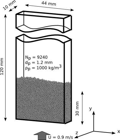
Figure 1: Geometry of the 3D computational domain for the simulation.

3.1 Solver Validations

The purpose of this validation is to show the results obtained from the proposed CFD–DEM solver are consistent with the experimental measurements and numerical simulations in the literature. The setup and parameters used in this validation test are detailed in Table 1. The mesh resolution used in this simulation is $N_{x}\times N_{y}\times N_{z}=36\times 100\times 8$, where $N_{x}$, $N_{y}$, and $N_{z}$ are the numbers of cells in the width ($x$-), height ($y$-), and transverse thickness ($z$-) directions, respectively.

The measurements of fluid volume fraction $\varepsilon_{f}$ in the experiments (Müller et al., 2009) were taken on two cross-sections at the heights $y=16.4$ mm and $y=31.2$ mm. To facilitate comparison with the experimental measurements, the profiles of $\varepsilon_{f}$ at the two heights are extracted in the present simulations. The comparison with the experimental data and the CFD–DEM simulations of Müller et al. (2009) are presented in Fig. 2. As can be seen from the figure, overall the $\varepsilon_{f}$ profiles predicted by the present CFD–DEM solver have favorable agreement with the experimental results and the numerical simulations of Müller et al. (2009). However, it is noted that both solvers predicted higher fluid volume fraction $\varepsilon_{f}$ near the boundaries (slippery walls) compared with experimental measurements. This is particularly prominent for location $y=31.2$ mm. As pointed out by Müller et al. (2009), the discrepancy in the $\varepsilon_{f}$ profiles is due to the over-prediction of the width of the bubbles in the CFD–DEM solvers, which consequently leads to higher $\varepsilon_{f}$ values near the wall. Since this over-prediction is attributed to the difficulty of the CFD–DEM framework in modeling the wall effects, and it is not directly related to our solver in particular, further discussions are not pursued here.

The vertical component $U_{y}$ of the time-averaged particle phase velocity are shown in Fig. 3, with comparisons among the current simulations, the experimental measurement, and the numerical simulations of Müller et al. The comparisons are presented for two cross-sections at the heights $y=15$ mm and $y=25$ mm, as these are the locations where experimental measurements were performed (Müller et al., 2008). It can be seen from Fig. 3 that generally speaking both CFD–DEM solvers give good predictions of the particle phase velocity $U_{y}$ for both locations, although arguably the prediction quality of our solver seems to be slightly better. Specifically, the simulations of Müller et al. tend to over-predict the particle velocities at both locations; while our simulations do not seem to have this issue except for a very minor over-prediction near the centerline (between $x=0.015$ m and $0.025$ m) for the profile at $y=15$ mm. On the other hand, the particle velocity $U_{y}$ near the centerline is under-predicted for $y=25$ mm. Overall, the magnitude of time-averaged particle velocity predicted by the present simulation using diffusion-based algorithm is smaller than that in the simulation of Müller et al. A possible explanation is the different solid volume fraction $\varepsilon_{s}$ fields used in the two solvers. The $\varepsilon_{s}$ field computed with the diffusion-based method is smoother and is thus free from very large $\varepsilon_{s}$ values. Since the computed drag force on a particle increases dramatically with the increase of $\varepsilon_{s}$, over-prediction of the drag forces on particles due to high $\varepsilon_{s}$ is more likely when the PCM coarse graining is used compared to the diffusion-based method. It is worth noting that one should not be deceived by the very similar averaged $\varepsilon_{s}$ profiles for both simulations in Fig. 2. In fact, the instantaneous $\varepsilon_{s}$ fields obtained with PCM have much more very larger values, as has been demonstrated in the a priori tests in Sun and Xiao (2014). Although present only in very few cells, these large values can have a significant impact on the particle velocities, since the drag force is a highly nonlinear function of $\varepsilon_{s}$. Consequently, this leads to larger fluid drag forces on the particles in the PCM-based CFD–DEM solvers, and thus larger averaged solid phase velocities in the results.

In summary, although some discrepancies exist between the prediction of $\varepsilon_{f}$ by the present CFD–DEM solver and the experimental results, the overall agreement is favorable. Moreover, the fluid volume fraction and particle phase velocities obtained in the present simulations are in very good agreement with the previous CFD–DEM simulations of the same case (Müller et al., 2008). Hence, the validations are deemed successful, and further investigations using the CFD–DEM solver are pursued below.

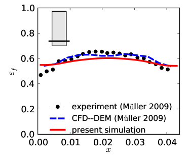
(a)

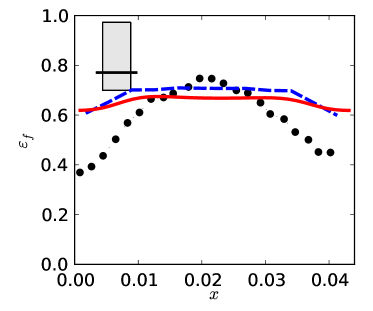
(b)

Figure 2: Profiles of time-averaged fluid volume fraction obtained from the present simulations compared with the experimental measurements and numerical simulation of Müller et al. (2009). The results are presented at two vertical locations: (a) $y=16.4$ mm and (b) $y=31.2$ mm.

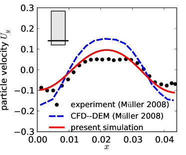
(a)

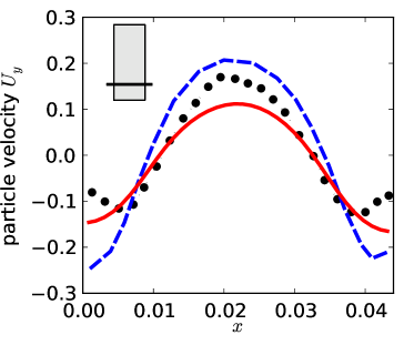
(b)

Figure 3: Profiles of time-averaged vertical velocity of particles obtained from the present simulation. The measurements are taken at different heights according to the experiment (Müller et al., 2008). (a) Particle velocity at the height of 15 mm, (b) particle velocity at the height of 25 mm.

3.2 Mesh-Independence Study of CFD–DEM simulations

In the a priori simulations presented in the companion paper (Sun and Xiao, 2014), it has been demonstrated that the diffusion-based method yields mesh-independent solid volume fraction fields. Here we further demonstrate that the CFD–DEM simulations with diffusion-based coarse graining give mesh-independent results. In particular, average particle phase velocities and fluid volume fraction at various locations are studied extensively and are compared among simulations performed on five successively refined meshes. To characterize the sizes of arbitrarily shaped cells, we use the parameter cell length scale $S_{c}$ defined as:

$$S_{c}=\sqrt[3]{V_{c}},$$ (10)

where $V_{c}$ is the volume of a cell. Five meshes A–E are used in the mesh-independence studies here with the effective lengths $S_{c}$ = $6d_{p}$ (mesh A), $4d_{p}$ (mesh B), $2d_{p}$ (mesh C), $d_{p}$ (mesh D), and $0.5d_{p}$ (mesh E), arranged with increasing mesh resolution. Larger $S_{c}$ values indicate larger cell sizes and thus coarser meshes. Details of the mesh parameters are presented in Table 2.

Table 2: Parameters in mesh-independence study of the CFD–DEM solvers with diffusion-based and PCM-based coarse-graining methods. The study using the solver with diffusion-based method covers a wider range of mesh resolutions, while meshes (e.g., D and E) with small cells cannot be used in the PCM-based solver due to instabilities.

mesh	$S_{c}/d_{p}$	$N_{x}$	$N_{y}$	$N_{z}$	used in
A	6	$6$	$16$	$1$	diffusion-based; PCM
B	4	$9$	$25$	$2$	diffusion-based; PCM
B′	3	$12$	$32$	$3$	PCM only
C	2	$18$	$50$	$4$	diffusion-based; PCM
D	1	$36$	$100$	$8$	diffusion-based only
E	0.5	$72$	$200$	$16$	diffusion-based only

As with the validation studies above, the fluid volume fractions $\varepsilon_{f}$ profiles at two cross sections at heights $y=16.4$ mm and $y=31.2$ mm are shown in Figs. 4(a) and 4(b). Moreover, the profiles of fluid volume fraction $\varepsilon_{f}$ at two vertical cross-sections at $x=11$ mm and $x=22$ mm (located at a quarter width location and at the centerline of the domain, respectively) are shown in Figs. 4(b) and 4(d). Although experimental data are not available at the two vertical cross-sections, this does not impair the objective of the mesh-convergence study, since we are mainly concerned with the comparison of results obtained with meshes with different coarseness levels, and not with the agreement between numerical predictions and experimental measurements. Examining the profiles at a few vertical cross-sections in addition to the horizontal cross-section locations helps shed light on the behavior of the result in the entire domain. To facilitate visualization, the locations of the corresponding cross-sections are indicated in the insets in the upper left corner of each plot along with the $\varepsilon_{f}$ profiles. The shaded regions in the insets indicate the initial particle bed. It can be seen that mesh convergence is achieved in the prediction of $\varepsilon_{f}$ as all meshes with $S_{c}/d_{p}$ smaller than 4 (e.g., meshes B, C, D, and E) give identical results. As to the $\varepsilon_{f}$ profiles obtained by using mesh A with $S_{c}/d_{p}=6$, some minor discrepancies with the converged results are observed, particularly in the region near the bottom inlet in Figs. 4(c) and  4(d). Since this mesh resolution is probably inadequate, the minor discrepancies are expected.

Similarly, the vertical component $U_{y}$ of the time-averaged particle phase velocity obtained at different horizontal and vertical cross-sections are shown in Fig. 5. Again, the general observation here is that the four finer meshes (B–D) all give identical results, indicating excellent mesh-convergence behavior, while some discrepancies are found in the results from mesh A ($S_{c}/d_{p}=6$). In contrast to the fluid volume fraction profiles shown in Fig. 4, the discrepancies between the results from mesh A and the converged results from meshes B–E occur mostly in the middle of the domain (e.g., between $x=0.01$ and $x=0.03$ in Figs. 5(a) and (b), and around $y=0.25$ in Figs. 5(c) and (d)).

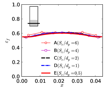
(a)

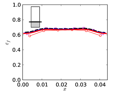
(b)

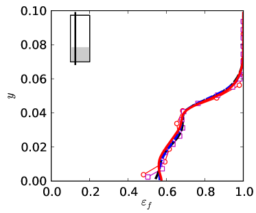
(c)

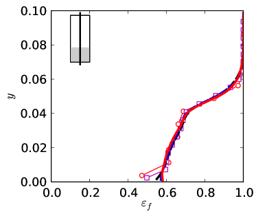
(d)

Figure 4: Mesh convergence study of the CFD–DEM solver with the diffusion-based coarse-graining method, showing the fluid volume fraction $\varepsilon_{f}$ ($=1-\varepsilon_{s}$) profiles on two horizontal cross-sections located at (a) $y=16.4$ mm and (b) $y=31.2$ mm, respectively, and two vertical cross-sections located at (c) $x=11$ mm and (d) $x=22$ mm, respectively. Insets in the panels show the location of the cross-section corresponding to each profile. The shaded regions in the inset indicates the initial particle bed. Results obtained based on five consecutively refined meshes are compared.

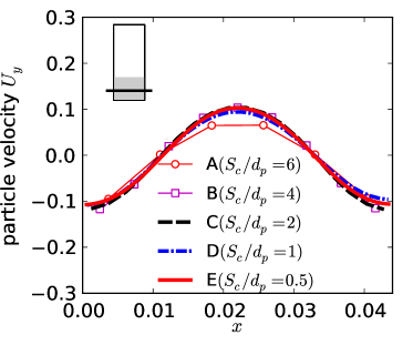
(a)

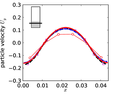
(b)

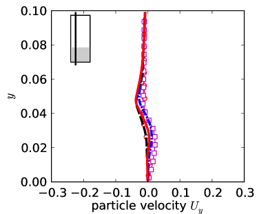
(c)

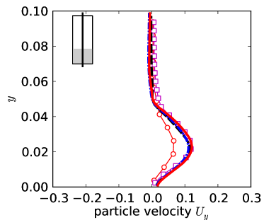
(d)

Figure 5: Mesh convergence study of the CFD–DEM solver with the diffusion-based coarse-graining method, showing the profiles of vertical component $U_{y}$ of the time-averaged particle velocity obtained on two horizontal cross-sections located at (a) $y=16.4$ mm and (b) $y=31.2$ mm, respectively, and two vertical cross-sections located at (c) $x=11$ mm and (d) $x=22$ mm, respectively. Insets in the panels show the locations of the cross-section corresponding to each profile. Results obtained based on five consecutively refined meshes are compared.

3.3 Performance Comparison with PCM

The mesh-convergence studies above demonstrated excellent mesh-convergence behavior of the CFD–DEM solver with diffusion-based coarse-graining method. To highlight this advantage, the same mesh-convergence study is performed on the CFD–DEM solver with PCM-based coarse-graining. All simulation setup and parameters are kept the same except for the coarse-graining method and the meshes used. Here only four meshes A ($S_{c}/d_{p}=6$), B ($S_{c}/d_{p}=4$), B^′ ($S_{c}/d_{p}=3$), and C ($S_{c}/d_{p}=2$) are used in the mesh-convergence study with PCM, since it is not possible obtain meaningful solid volume fraction field on meshes D ($S_{c}/d_{p}=1$) and E ($S_{c}/d_{p}=0.5$), which have cell length scales $S_{c}$ equal or smaller than the particle diameter. Even by capping the $\varepsilon_{s}$ field at 0.7 (detailed below), we were not able to complete simulations on meshes D or E without being interrupted by instabilities.

The profiles of time-averaged fluid volume fraction $\varepsilon_{f}$ obtained by using the same CFD–DEM solver with PCM-based coarse-graining method are shown in Fig. 6. Profiles at the same four cross-section as in Fig. 4 are presented. As can be seen from Fig. 6, at all cross-sections the $\varepsilon_{f}$ profiles obtained with meshes B ($S_{c}/d_{p}=4$) and B^′ ($S_{c}/d_{p}=3$) are the same, indicating an approximate mesh-independence. As with the results from the diffusion-based coarse-graining in Fig. 4, the results obtained with mesh A ($S_{c}/d_{p}=6$) have some discrepancies with the other results due to the inadequate mesh resolution. While this is not evident in Figs. 6(a) and 6(b), it can be seen at several locations in Figs. 6(c) and 6(d). Note that the deviations do not necessarily occur near the bottom boundary as in Figs. 4(c) and (d), but at random locations instead. Perhaps the most striking difference in the results in Fig. 6 is that the convergence is not achieved when the mesh is further refined, as is evident from the fact the results of mesh C ($S_{c}/d_{p}=2$) are different from those of meshes B and B^′. With mesh C, unphysically large $\varepsilon_{s}$ values are frequently encountered during the simulations, which cause instabilities. To address this issue associated with the PCM, a frequently used technique that is adopted here is “capping”, i.e., for all cells with solid volume fraction $\varepsilon_{s}$ larger than a certain threshold value, e.g., $\varepsilon_{\textrm{threshold}}=0.7$, the $\varepsilon_{s}$ in these cells are capped to be $\varepsilon_{\textrm{threshold}}$. This is done at each fluid time step after the $\varepsilon_{s}$ field is calculated. This technique improves the robustness of CFD–DEM simulations with PCM-based coarse graining, but it may impair the accuracy of the fluid drag calculation and the accuracy of the entire simulation, as an artificially set $\varepsilon_{s}$ value is used instead of the physical values in these cells. The capping technique may have caused the failure of mesh-convergence observed in Fig. 6. The particle phase velocities obtained on meshes A, B, B^′, and C with the PCM-based solver are presented in Fig. 7. Similar to what was observed in Fig. 6, mesh-convergence is not achieved here, mainly due to the fact that mesh C produces result different from those of meshes B and B^′. The discrepancies are most evident from Figs. 7(c) and (d). In Fig. 7(d), it can be seen that even the results obtained with meshes B and B^′ are different.

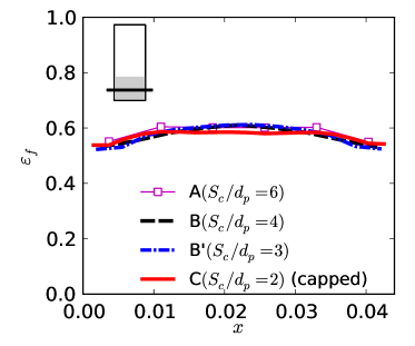
(a)

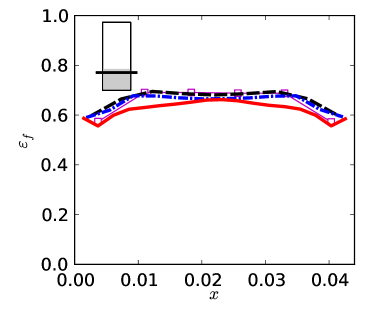
(b)

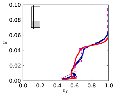
(c)

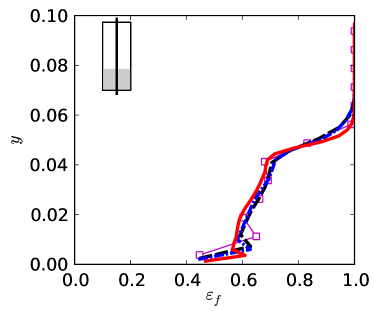
(d)

Figure 6: Mesh convergence of PCM-based coarse graining, showing the profiles of fluid volume fraction $\varepsilon_{f}$ ($=1-\varepsilon_{s}$) on cross-sections at (a) $y=16.4$ mm, (b) $y=31.2$ mm, (c) $x=11$ mm, and (d) $x=22$ mm. Results from four meshes A, B, B^′, and C are compared. Refer to Fig. 4 for detailed caption and for comparison.

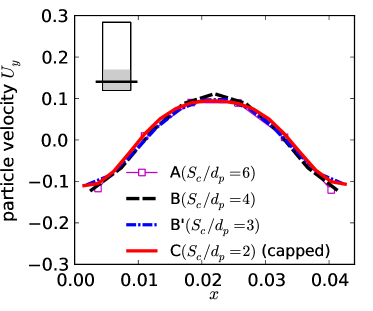
(a)

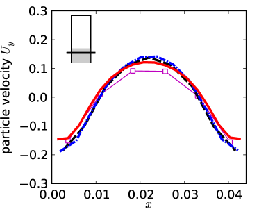
(b)

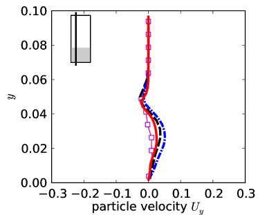
(c)

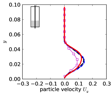
(d)

Figure 7: Mesh convergence of PCM-based coarse graining, showing the profiles of vertical component $U_{y}$ of the time-averaged particle velocity at (a) $y=15$ mm, (b) $y=25$ mm, (c) $x=11$ mm, (d) $x=22$ mm. Results from four meshes A, B, B^′, and C are compared. Refer to Fig. 5 for detailed caption and for comparison.

To further compare the different effects of the two coarse-graining methods on the CFD–DEM results, snapshot sequences of particle locations during a bubble evolution cycle are presented in Fig. 8. The results from mesh C ($S_{c}/d_{p}=2$) are presented here, since the mesh-convergence study above seems to suggest this to be a suitable mesh for both cases. The snapshots at $t=0.00$ s correspond to the beginning of the cycle. The volume fraction contours corresponding to $\varepsilon_{s}=0.28$ are overlaid on top of the particle location plots to separate regions of lower and higher solid volume fractions, which facilitate visualization of the bubble shapes and locations. This contour value 0.28 is chosen to be one half of the maximum solid volume fraction in the initial bed configuration. From Fig. 8(a), the bubble formation ($t=0.04$ s), growth ($0.08$ s), and burst ($0.12$ s) can be clearly identified. At $t=0.12$ s, when the upper bubble bursts, a small bubble formed near the bottom of the bed. In the subsequent snapshots from $0.16$ s to $0.24$ s, the bubble rises and grows until it reaches the top of the bed at $0.28$ s, and bursts at $0.32$s eventually. The bubble dynamics observed here is physically reasonable as confirmed in previous experiments (Müller et al., 2008) and numerical simulations (Peng et al., 2014). In contrast, in the results obtained by using the same CFD–DEM solver but with PCM-based coarse-graining, which is shown in Fig. 8(b), the cycle of bubble formation, growth, and bursting are not observed as clearly, although the sequence from 0.04 s to 0.12 s does vaguely show a similar bubble evolution dynamics as in Fig. 8(a). Moreover, the bubble shapes in the PCM results are much more irregular than those observed in the diffusion-based results. To further illustrate the different bubble dynamics, snapshots of solid volume fractions of the same cycle are shown in Fig. 9(a) and (b) for the CFD–DEM solvers with diffusion-based and PCM-based coarse graining, respectively. In Fig. 9(a) the same sequence of bubble dynamics as explained above are observed. The bubbles can be clearly identified from the snapshots of solid volume fractions. On the other hand, in the PCM results shown in Fig. 9(b), the bubbles are not as easily identified, which is partly due to the large local variations (i.e., spatial gradients) in the $\varepsilon_{s}$ field.

In summary, with the same mesh, computational setup, parameters, and CFD–DEM solver but only with different coarse-graining methods, the two carefully designed test cases clearly suggest the superiority of the diffusion-based method compared with the PCM-based method in obtaining CFD–DEM simulation results with mesh-convergence and in capturing the physics of the bubble dynamics in the fluidized bed.

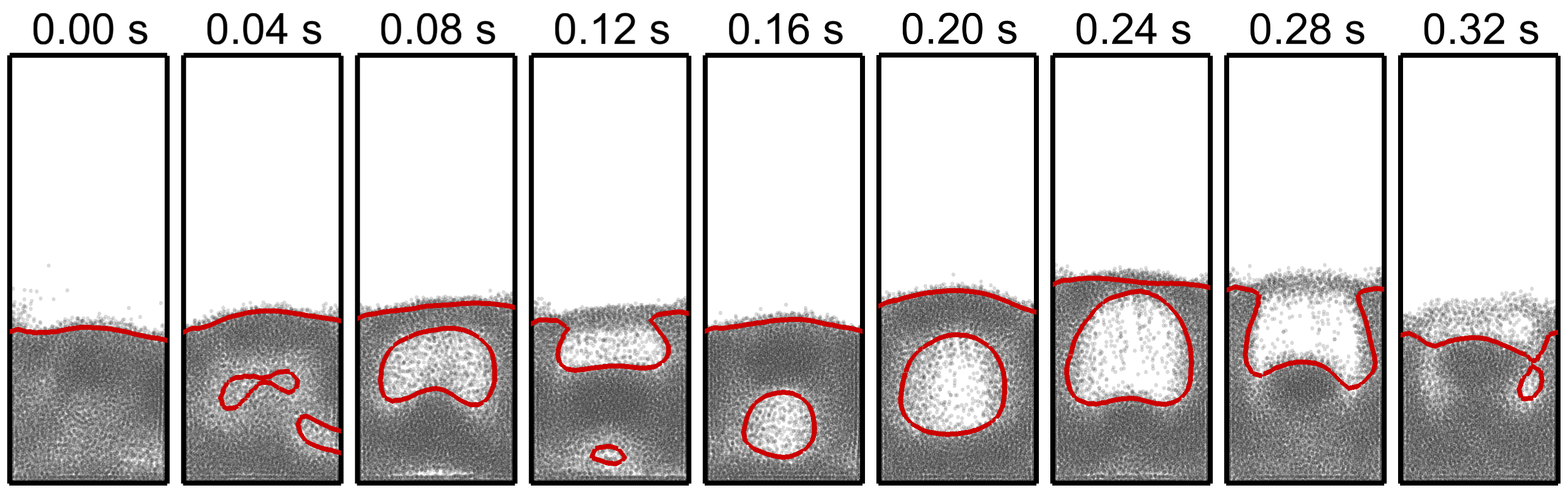
(a)

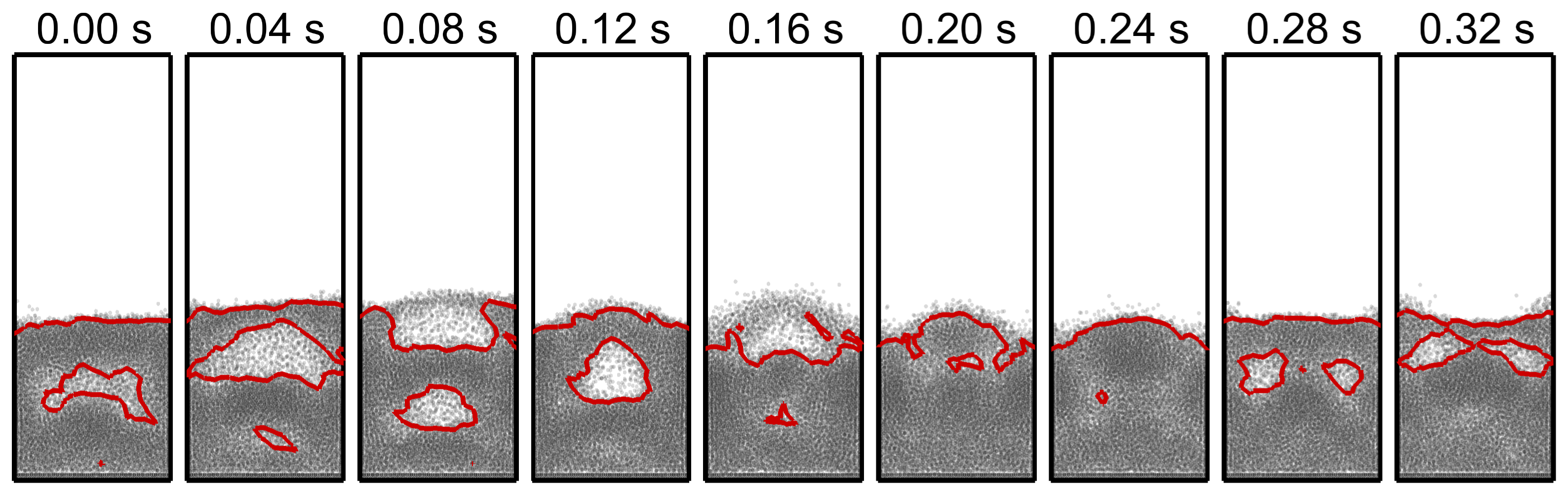
(b)

Figure 8: Snapshots of particle locations during a cycle of bubble formation and evolution, showing the results obtained by using the CFD–DEM solver with (a) diffusion-based and (b) PCM coarse-graining methods. The overlaying contours corresponds to $\varepsilon_{s}=0.28$, which is half of the maximum $\varepsilon_{s}$ value in the initial bed configuration. The time origin ($t=0$ s) corresponds to the beginning of the cycle.

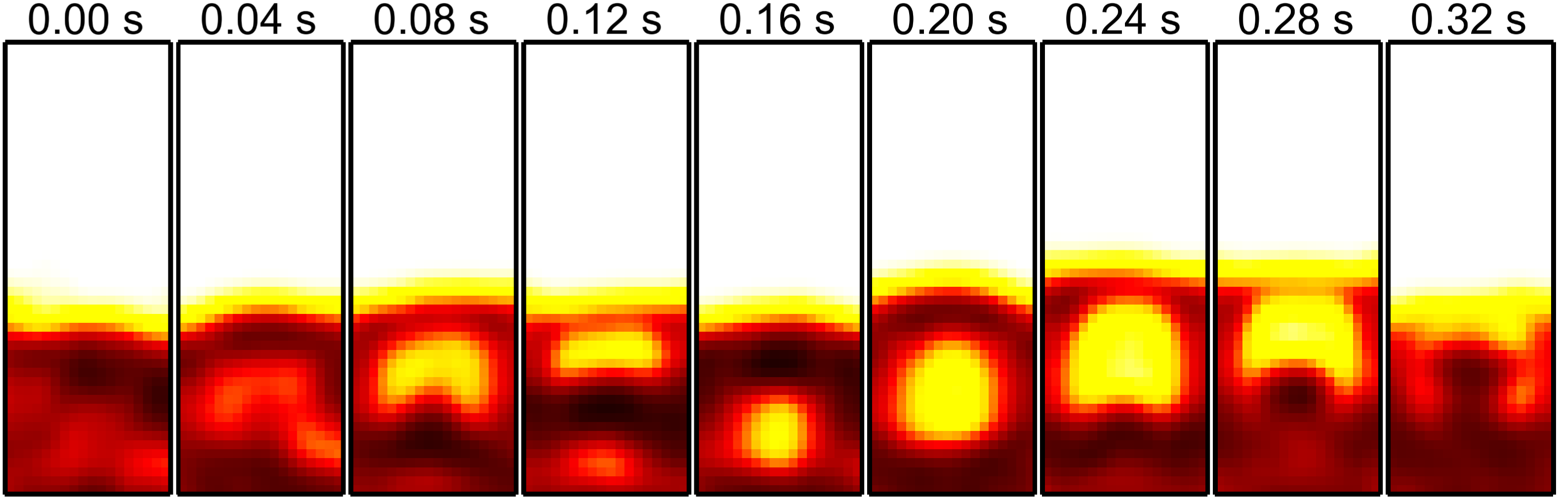
(a)

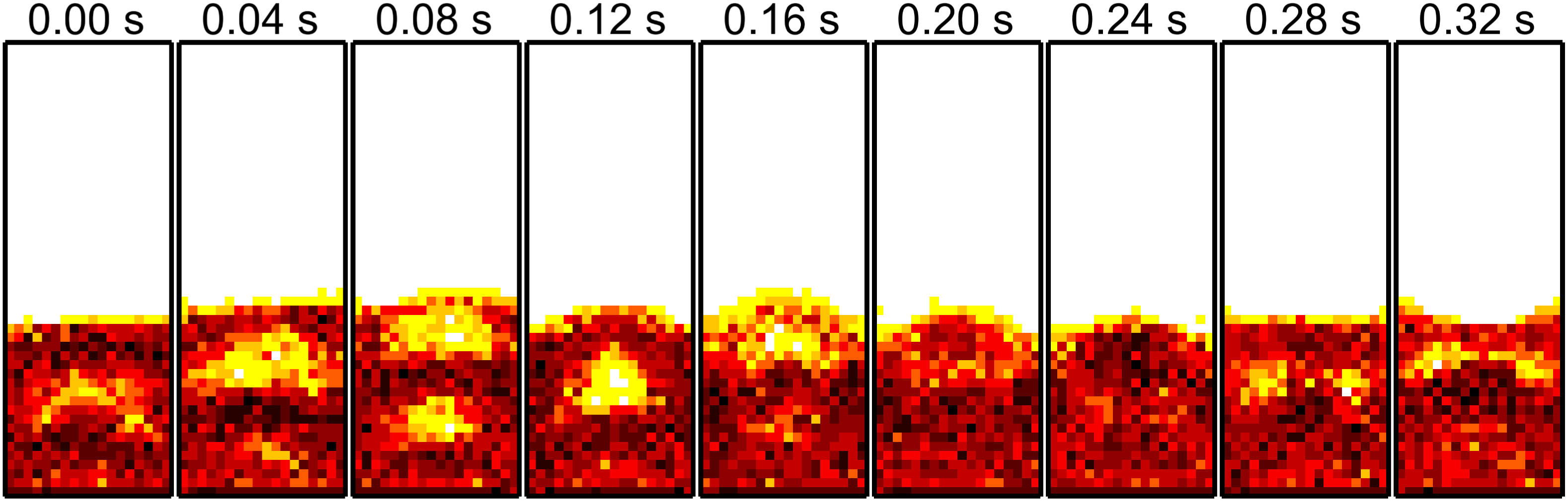
(b)

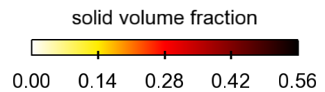
(c)

Figure 9: Snapshots of solid volume fraction $\varepsilon_{s}$ during a cycle of bubble formation and evolution, showing the results obtained by using the CFD–DEM solver with (a) diffusion-based and (b) PCM coarse-graining methods. The time origin ($t=0$ s) corresponds to the beginning of the cycle.

3.4 Computational Overhead of Diffusion-Based Coarse Graining

In a typical CFD–DEM solver, the computational cost of DEM simulation dominates due to the high computational costs in resolving particle collisions and the small time-scales in these particle-scale processes. In contrast, the number of cells in the CFD mesh and the associated computational cost for the CFD simulation are generally moderate, since the cells must be large enough to contain a sufficient number of particles for the locally averaged Navier–Stokes equations to be valid. Since the diffusion equations are solved on the CFD mesh, the computational cost associated with the diffusion-based coarse graining is of the same order as that of the CFD simulation. Therefore, the additional computational costs incurred by solving the diffusion equation are unlikely to be a significant portion of the entire CFD–DEM simulation. In LES–DEM, however, the number of cells in the LES mesh may be large, and thus the computational overhead due to the coarse-graining procedure based on solving diffusion equations may become a concern. To minimize the computational overhead, an implicit time stepping scheme should be used to guarantee stability, which allows for large time step sizes to be used in the solution of the coarse-graining diffusion equations. In Sun and Xiao (2014) we have shown that with any reasonable bandwidth the diffusion equation can be solved with one time step to obtain sufficient accuracy, although some minor fluctuations are still present in the coarse-grained field. If the diffusion equation is solved with three time steps, the obtained field is sufficiently smooth, at least compared with those obtained by using PCM and DPVM.

To investigate the computational costs associated with different parts of a typical CFD–DEM simulation, a series of four numerical simulations are performed with the ratio $N_{p}/N_{c}$ between the number $N_{p}$ of particles and the number $N_{c}$ of CFD cells varying from 2 to 16. In these cases the number of particles $N_{p}$ is kept constant at $3.32\times 10^{5}$, while the numbers of CFD cells $N_{c}$ vary from $2.1\times 10^{4}$ to $1.7\times 10^{5}$. The computational cases are constructed according to those presented in Section 3, except that the computational domain is enlarged to $264$ mm $\times~{}120$ mm $\times~{}60$ mm (in the width $x$-, height $y$-, and transverse thickness $z$-directions, respectively) to allow for a realistically large number of cells and particles to be used. As in the experiment, the initial bed height is set to $30$ mm to retain the same bed dynamics as in the experiment, but note that both the width and the transverse thickness have been increased by six times. Since the CPU time needed for each time step is relatively constant throughout the entire simulation, only 100 fluid time steps are simulated in these tests.

The CPU times consumed by different parts of the CFD–DEM simulations, including the CFD part, the DEM part, and the coarse graining part (mainly the solution of the diffusion equations), are presented in Table 3 for the four cases studies. It can be seen from the table that the total time spent on the DEM part do not vary much among the four cases, which is expected since the total number of particles are the same in all the cases. On the other hand, the time spent on the CFD part and that on the coarse graining increases as the number of CFD cells increases, at a rate slightly higher than linear. It is worth noting that in all these cases the time spent on coarse graining is slightly longer than the CFD part. This is because the coarse graining diffusion equations are performed for seven fields associated with three variables $\varepsilon_{s}$, $u_{i}$, $F_{i}$ in each fluid time step. Three times steps are used each time when these equations are solved. However, note that the percentage of CPU time spent on the coarse graining decreases with increasing ratio $N_{p}/N_{c}$. Even for case 1 with $N_{p}/N_{c}=2$, which indicates that there are only two particles for each cell on average, the coarse graining accounts for only 28% of the total computational cost. Considering that the number of particles relative to the number of cells is very small, this percentage is not really discouraging. Peng et al. (2014) pointed out that a cell size of $1.63d_{p}$ is needed to satisfy the CFD–DEM governing equations. A rule of thumb for CFD–DEM simulations is that on average a typical cell should contain approximately nine particles (Müller et al., 2009; Xiao and Sun, 2011). In view of these observations, cases 3 and 4 are probably more realistic in terms of $N_{p}/N_{c}$ ratios. In the two cases, the diffusion-based coarse-graining procedure accounts for only 10% and 5%, respectively, of the total cost of the CFD–DEM simulations, which we believe are rather moderate. Admittedly, the diffusion equations incur more computational costs than the CFD solver. This is in stark contrast to PCM and DPVM, which are expected to incur negligible computational costs. The computational overhead of the diffusion-based method may be significant and undesirable when fine meshes are used, i.e., when high-resolution solvers such as LES are used in the CFD part. In these cases, one may consider further increasing the time step size used in solving the diffusion equations, e.g., solving the diffusion equation in only one time step with an implicit scheme (see Sun and Xiao, 2014). Alternatively, one can recast the continuity equation (2a) to eliminate the term $\varepsilon_{s}\mathbf{U}_{s}$ (see Eq. (1a) in Wu et al. (2014)), so that the number of diffusion equations to solve is reduced from seven to four.

A few additional observations need to be made when examining the computational overhead due to the diffusion-based coarse-graining procedure. First, we have demonstrated in the companion paper (Sun and Xiao, 2014) that even on unfavorable meshes the diffusion-based coarse-graining method lead to smooth solid volume fraction $\varepsilon_{s}$ fields (as well as $\mathbf{U}_{s}$ and $\mathbf{F}^{fp}$). As observed by Peng et al. (2014), compared to the non-smooth coarse grained fields (e.g., $\varepsilon_{s}$) such as those obtained by using the PCM, a smooth $\varepsilon_{s}$ field can significantly accelerate convergence in the CFD solver, and thus effectively reduces overall computational costs of the CFD–DEM simulation. Second, the parallelization of the diffusion-based method is straightforward and can very effectively take advantage of exiting infrastructure in the CFD solver, which is often highly optimized. The two factors partly offset the moderate computational overhead associated with the diffusion-based coarse-graining procedure. On the other hand, as demonstrated in previous studies (Wu et al., 2006, 2009a; Xiao and Sun, 2011), linearization and implicit treatment of the fluid–particle momentum exchange terms are effective methods for accelerating the convergence of the PISO algorithm by increasing the diagonal dominance in the matrix of the discretized linear equations systems. Diffusing the fluid–particle drag forces as performed in the proposed method makes it difficult, if not impossible, to perform such linearizations. This is a potential limitation of the diffusion-based coarse-graining method if linearization and implicit treatment are essential, e.g., in such challenging cases as granular Rayleigh-Taylor instability problems (Wu et al., 2014).

Table 3: Breakdown of computational costs associated with different parts of CFD–DEM simulations. The computational costs are presented for four cases with the same number of particles $N_{p}=3.3\times 10^{5}$ and different numbers $N_{c}$ of CFD cells. The CPU times presented here are normalized by the time spent on the CFD part of case 4, which has the smallest number of CFD cells.

case	$N_{c}$	$N_{p}/N_{c}$	CFD	DEM	coarse graining
1	$1.7\times 10^{5}$	2	$12~{}(23\%)$	$26~{}(49\%)$	$14.8~{}(28\%)$
2	$8.3\times 10^{4}$	4	$~{}5~{}(13\%)$	$27~{}(70\%)$	$~{}6.4~{}(17\%)$
3	$4.1\times 10^{4}$	8	$~{}2~{}(~{}7\%)$	$25~{}(83\%)$	$~{}2.8~{}(10\%)$
4	$2.1\times 10^{4}$	16	$~{}1~{}(~{}3\%)$	$27~{}(92\%)$	$~{}1.5~{}(~{}5\%)$

4 Discussion

4.1 Choice of Bandwidth in Kernel Functions for Coarse Graining

In coarse-graining procedures used to link microscopic and macroscopic quantities, the choice of parameters (e.g., the bandwidth $b$ in the kernel functions) remains an open question (Lätzel et al., 2000; Zhu and Yu, 2002). Here we argue that in CFD–DEM simulations the bandwidth $b$ should be chosen based on the size of the wake of the particles in the fluid flow, which in turn depends on the particle diameter and the particle Reynolds number, among other parameters (Wu and Faeth, 1993). While coarse graining may be performed for different theoretical and practical purposes depending on the physical context, in CFD–DEM the main reason for the coarse graining is to compute the interactions forces between the fluid and the particle phases. Specifically, for example, the solid volume fraction $\varepsilon_{s}$ is needed in the drag force calculation to account for the effects of a particle on the drag experienced by other particles. It is also needed in the continuity and momentum equations of the fluid phase. In the latter, in addition to $\varepsilon_{s}$ and $\mathbf{U}_{s}$, which are obtained via coarse graining, the force of a particle on the fluid needs to be distributed to an appropriate volume of the fluid. In light of this observation, from a physical perspective the support of the kernel function should extend approximately to the same distance as the wake of the particles. The wake size depends on the particle Reynolds number, which in turn depends on the relative velocity between the particle and the fluid. To compute the wake size of the particles (indicated by the velocity defect along the particle centerline) in the case studied in Section 3, a few representative relative velocity values are used, and the results are displayed in Fig. 10.

A bandwidth between $b=4d_{p}$ and $6d_{p}$ was used in the simulations in the current work (Section 3) and in the a priori tests in the companion paper (Sun and Xiao, 2014). Since the support of the kernel is approximately $3b$, this choice of bandwidth corresponds to a kernel support of approximately 12 to 18 particle diameters. This is indeed of the same order of magnitude as that suggested by the wake sizes shown in Fig. 10. In a polydispersed system with a range of particle diameters, although changing bandwidth $b$ (or equivalently diffusion time span $T$) adaptively according to relative particle velocities would be unrealistic and probably unnecessary as well, it is possible and easy to accommodate different particles sizes (and thus wake sizes) by using a spatially varying diffusion coefficient in Eq. (5a). Currently, a diffusion coefficient that is uniformly one is used throughout the domain.

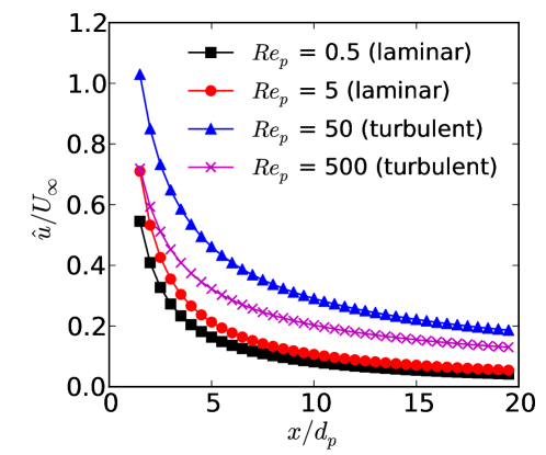
Figure 10: Velocity defect $\hat{u}\equiv U_{\infty}-u$ normalized by the free-stream velocity $U_{\infty}$ in the wake of a spherical particle along the imaginary streamline passing through the center of the sphere, illustrating the size of the wake of a particle at different flow regimes and particle Reynolds numbers, which are defined as $Re_{p}=U_{\infty}d_{p}/\nu_{f}$ (where $\nu_{f}$ is the fluid kinematic viscosity). Results are obtained according to the empirical formulas in Wu and Faeth (1993) and are presented for a range of typical particle Reynolds numbers. To obtain these $Re_{p}$ values, particle–fluid relative velocities $U_{\infty}$ ranging from 0.005 m/s to 5 m/s, a particle diameter of $d_{p}=1$ mm, and a fluid viscosity of $\nu_{f}=1.0\times 10^{-6}~{}\mathrm{m^{2}/s}$ are used.

4.2 Implementation of Time–Volume Averaging in CFD–DEM Solvers

As with most previous CFD–DEM works, in this study we consider only volume averaging in the coarse graining procedure. That is, the kernel $G(\mathbf{x})$ is a spatial function, and it operates on particle distributions at a particular time only. Accordingly, the diffusion equation as in Eq. (5a) is solved only to smoothen the coarse-grained fields at each time fluid step. Note that the time variable $\tau$ in the diffusion equation is the pseudo-time, and not the physical time. In principle it is possible to include time in the kernel function as well, i.e., $G=G(\mathbf{x},t)$, with the normalization condition revised to be $\int_{\mathbb{R}^{4}}G(\mathbf{x},t)d\mathbf{x}dt=0$. This is indeed what was proposed in Zhu and Yu (2002). However, the kernel function $G(\mathbf{x},t)$ is symmetric both spatially and temporally. Essentially, the solid volume fraction $\varepsilon_{s}$ at any location is contributed to by particles in its surroundings in all directions, with closer particles having more contributions. Similarly, $\varepsilon_{s}$ depends on the particle distributions at both past and future times. This spatial and temporal symmetry is desirable from a theoretical point of view. However, in CFD–DEM solvers a kernel function with the symmetry in time cannot be implemented, since at time $t$ when we need to compute $\varepsilon_{s}(x,t)$ the particle distributions at future times are not known but need to be solved. If coarse graining or averaging in time is indeed desirable or necessary (e.g., when the flow fields have high-frequency fluctuations such as in LES–DEM), an alternative to obtain a field with time–volume averaging, e.g., $\left<\varepsilon_{s}(\mathbf{x},t)\right>$, is to use a single-sided averaging scheme as follows (Meneveau et al., 1996; Xiao and Jenny, 2012):

$$\left<\varepsilon_{s}(\mathbf{x},t)\right> =\int_{0}^{t}\varepsilon_{s}(\mathbf{x},t^{\prime})W(t-t^{\prime})dt^{\prime}$$ (11)

$$\textrm{with}\quad W(t-t^{\prime}) =\frac{1}{b_{t}}\exp\left[-(t-t^{\prime})/b_{t}\right],$$

where $\varepsilon_{s}$ is the solid volume fraction with volume averaging only, $W$ is the exponential kernel function, and $b_{t}$ is the temporal averaging bandwidth with similar interpretation to $b$ in Eq. (6). Compared with the Gaussian kernel function, a convenient feature of the exponential kernel function is that $\left<\varepsilon_{s}\right>$ as defined in Eq. (11) is the solution of the following differential equation:

$$\frac{d\left<\varepsilon_{s}\right>}{dt}=\frac{1}{b_{t}}(\varepsilon_{s}-\left<\varepsilon_{s}\right>),$$ (12)

which can be approximated to the first order by the following relation:

$$\left<\varepsilon_{s}\right>^{n} =(1-\alpha)\varepsilon_{s}^{n}+\alpha\left<\varepsilon_{s}\right>^{n-1}$$ (13)

$$\textrm{with}\quad\alpha =\frac{1}{1+\Delta t/b_{t}},$$ (14)

where $n$ and $n-1$ are the time indices of the present and the previous time steps, respectively. The scheme in Eq. (13) suggests that to compute $\left<\varepsilon_{s}\right>$ for the current step, one only needs $\varepsilon_{s}$ of the current step and $\left<\varepsilon_{s}\right>$ of the previous time step. This would lead to reduced storage requirements compared with a literal implementation of Eq. (11), where $\varepsilon_{s}$ at many previous time steps need to be stored. While the above-mentioned characteristics of exponential kernel function are exploited in the averaging in turbulence flow simulations (Meneveau et al., 1996; Xiao and Jenny, 2012), we are not aware of any such attempts in the context of coarse graining in CFD–DEM simulations. Hence, we chose to present it here for the completeness of the diffusion-based coarse-graining algorithm and for the reader’s reference.

5 Conclusion

In this work we applied the previously proposed coarse-graining algorithm based on solving diffusion equations (Sun and Xiao, 2014) to CFD–DEM simulations. The conservation requirements are examined and satisfied by properly choosing variables to solve diffusion equations for. Subsequently, the algorithm is implemented into a CFD–DEM solver based on OpenFOAM and LAMMPS, the former being a general-purpose, three-dimensional, parallel CFD solver based on unstructured meshes. The implementation is straightforward, fully utilizing the computational infrastructure provided by the CFD solver, including the parallel computing capabilities. Simulations of a fluidized bed showed that the diffusion-based coarse-graining method led to more robust simulations, physically more realistic results, and improved ability to handle small CFD cell-size to particle-diameter ratios. Moreover, the mesh convergence characteristics of the diffusion-based method are dramatically improved compared with the PCM. It is demonstrated in the current work that the diffusion-based method lead to mesh-independent results in CFD–DEM simulations, confirming the conclusions drawn from the a priori tests in the companion paper (Sun and Xiao, 2014). The choice of the computational parameter, i.e., the bandwidth, has clear physical justifications. The computational costs of the proposed method were carefully investigated. Results suggest that, although the computational overhead due to the diffusion-based coarse graining exceeded that of the CFD solver in all cases, the additional computational costs are not significant (less than 10% of the total costs) if the number of particles per cell is large, i.e., when the computational costs of the simulations are dominated by the DEM part. Therefore, the diffusion-based method is a theoretically elegant and practically viable option for coarse graining in general-purpose CFD–DEM solvers.

6 Acknowledgment

The computational resources used for this project were provided by the Advanced Research Computing (ARC) of Virginia Tech, which is gratefully acknowledged. We thank the anonymous reviewers for their comments, which helped improving the quality of the manuscript.

Appendix A Conservation Characteristics of the Diffusion-Based Method

The conservation requirements for the particle mass, particle momentum, total momentum in the fluid–particle system as specified in Section 2.2.2 are summarized as follows:

$$\rho_{s}\sum_{k=1}^{N_{c}}\varepsilon_{s,k}\,V_{c,k} =\sum_{i=1}^{N_{p}}\rho_{s}\,V_{p,i}\;,$$ (15a)

$$\rho_{s}\sum_{k=1}^{N_{c}}\varepsilon_{s,k}\,V_{c,k}\,\mathbf{U}_{s,k} =\sum_{i=1}^{N_{p}}\rho_{s}\,V_{p,i}\,\mathbf{u}_{p,i}\;,$$ (15b)

$$\sum_{k=1}^{N_{c}}(1-\varepsilon_{s,k})\rho_{f}\,V_{c,k}\,\mathbf{F}^{fp}_{k} =-\sum_{i=1}^{N_{p}}\,\mathbf{f}^{fp}_{i}\;,$$ (15c)

where the density $\rho_{s}$ is assumed to be constant for all particles; $N_{c}$ is the number of cells in the CFD mesh; $N_{p}$ is the number of particles in the system; $V_{c,k}$ is the volume of cell $k$; $\mathbf{U}_{s,k}$ is the Eulerian solid phase velocity in cell $k$; $\mathbf{u}_{p,i}$ is the Lagrangian velocity of particle $i$; $\mathbf{F}^{fp}_{k}$ is the force per unit fluid mass exerted on fluid cell $k$ by all particles; $\mathbf{f}^{fp}_{i}$ is the fluid force on particle $i$.

Multiplying both sides of the equations in the PCM coarse-graining procedure, i.e., Eqs. (4),  (7), and (8), by $V_{c,k}$, $\rho_{s}\varepsilon_{s,k}V_{c,k}$, and $\rho_{f}\varepsilon_{f,k}V_{c,k}$, respectively, and taking summation over all cells, the conservation requirements in Eq. (15) can be recovered. Therefore, the PCM-based coarse-graining schemes as in Eqs. (4),  (7), and (8) are conservative by construction. The proposed coarse-graining algorithm consists of two steps: (1) coarse graining using PCM; and (2) solving diffusion equations for the quantities $\varepsilon_{s}$, $\varepsilon_{s}\mathbf{U}_{s}$ and $\varepsilon_{f}\mathbf{F}^{fp}$. Hence, for the proposed algorithm to be conservative, the diffusion step must also conserve the required physical quantities in the domain, i.e.,

$$\textrm{particle mass}:\quad \rho_{s}\sum_{k=1}^{N_{c}}\varepsilon_{s,k}\,V_{c,k}\;,$$ (16a)

$$\textrm{particle momentum}:\quad \rho_{s}\sum_{k=1}^{N_{c}}\varepsilon_{k}\,V_{c,k}\,\mathbf{U}_{s,k}\;,\;$$ (16b)

$$\textrm{total momentum of fluid--particle system}:\quad \rho_{f}\sum_{k=1}^{N_{c}}\varepsilon_{f,k}\,V_{c,k}\,\mathbf{F}^{fp}_{k}\;.$$ (16c)

For the diffusion equation ${\partial\phi}/{\partial t}=\nabla^{2}\phi$ of a generic variable $\phi$ on domain $\Omega$ with no-flux condition $\partial\phi/\partial n=0$ on the boundaries $\partial\Omega$, integrating the equation on $\Omega$ yields:

$$\int\limits_{\Omega}\frac{\partial\phi}{\partial t}d\Omega=\int\limits_{\Omega}\nabla^{2}\phi d\Omega=\int\limits_{\partial\Omega}\nabla\phi\cdot d\mathbf{S} =0,$$ (17a)

$$\textrm{or equivalently,}\quad\frac{\partial}{\partial t}\int\limits_{\Omega}\phi d\Omega =0,$$ (17b)

which suggests that the conserved quantity that is implied by the diffusion equation ${\partial\phi}/{\partial t}=\nabla^{2}\phi$ is

$$\int_{\Omega}\phi\,d\Omega,$$ (18)

or

$$\sum_{k=1}^{N_{c}}\phi_{i}V_{c,k}$$ (19)

on a discretized finite volume mesh. Comparing Eq. (19) with the quantities in Eq. (16) suggests that diffusion equations should be solved for the following three quantities:

$$\varepsilon_{s},\quad\varepsilon_{s}\mathbf{U}_{s},\quad\textrm{ and }\quad\varepsilon_{f}\mathbf{F}^{fp}$$ (20)

to satisfy the conservation requirements for particle mass, particle momentum, total momentum in the fluid–particle system, respectively.

References

- Anderson and Jackson (1967) Anderson, T., Jackson, R., 1967. A fluid mechanical description of fluidized beds: Equations of motion. Industrial and Chemistry Engineering Fundamentals 6, 527–534.
- Ball and Melrose (1997) Ball, R. C., Melrose, J. R., 1997. A simulation technique for many spheres in quasi-static motion under frame-invariant pair drag and Brownian forces. Physica A: Statistical Mechanics and its Applications 247 (1), 444–472.
- Cundall and Strack (1979) Cundall, P., Strack, D., 1979. A discrete numerical model for granular assemblies. Géotechnique 29, 47–65.
- Dawson (1983) Dawson, J. M., 1983. Particle simulation of plasmas. Reviews of Modern Physics 55 (2), 403–447.
- Deb and Tafti (2013) Deb, S., Tafti, D. K., 2013. A novel two-grid formulation for fluidparticle systems using the discrete element method. Powder Technology 246, 601–616.
- Di Felice (1994) Di Felice, R., 1994. The voidage function for fluid-particle interaction systems. International Journal of Multiphase Flow 20 (1), 153–159.
- Glasser and Goldhirsch (2001) Glasser, B. J., Goldhirsch, I., 2001. Scale dependence, correlations, and fluctuations of stresses in rapid granular flows. Physics of Fluids 13 (2), 407–420.
- Gupta et al. (2013) Gupta, P., Ebrahimi, M., Robinson, M., Crapper, M., Sun, J., Ramaioli, M., Luding, S., Ooi, J., 2013. Comparison of coupled CFD–DEM and SPH–DEM methods in single and multiple particle sedimentation test cases. In: PARTICLES. September 18–20, Stuttgart, Germany.
- Gupta et al. (2011a) Gupta, P., Sun, J., Ooi, J., 2011a. Segregation studies in bidisperse fluidsed beds: CFD–DEM approach with DNS based drag force models. In: UK–China Particle Technology Forum. July 3–6, Birmingham, UK.
- Gupta et al. (2011b) Gupta, P., Sun, J., Ooi, J., 2011b. Study of drag force models in simulation of bidisperse gas–solid fluidised beds using a CFD–DEM approach. In: The 8th European Congress of Chemical Engineering. September 25–29, Berlin, Germany.
- Gupta et al. (2012) Gupta, P., Sun, J., Ooi, J., 2012. Effect of hydrodynamic interactions on the segregation rate in bi-disperse gas–solid fluidised bed and validation studies. In: 7th International Conference for Conveying and Handling of Particulate Solids – CHoPS. September 10–13, Friedrichshafen, Germany.
- Gupta et al. (2011c) Gupta, P., Xiao, H., Sun, J., 2011c. Effect of drag force models on simulation of segregation in gas–solid fluidised beds using a CFD–DEM approach. In: UK–China Particle Technology Forum. July 3–6, Birmingham, UK.
- Han et al. (2007) Han, K., Feng, Y. T., Owen, D. R. J., 2007. Numerical simulations of irregular particle transport in turbulent flows using coupled LBM-DEM. Computer Modeling in Engineering and Sciences 18 (2), 87–100.
- Issa (1986) Issa, R. I., 1986. Solution of the implicitly discretised fluid flow equations by operator-splitting. Journal of Computational Physics 62 (1), 40–65.
- Iverson (1997) Iverson, R. M., 1997. The physics of debris flows. Reviews of Geophysics 35 (3), 245–296.
- Jasak (1996) Jasak, H., 1996. Error analysis and estimation for the finite volume method with applications to fluid flows. Ph.D. thesis, Imperial College London (University of London).
- Kafui et al. (2002) Kafui, K., Thornton, C., Adams, M., 2002. Discrete particle–continuum fluid modelling of gas–solid fluidised beds. Chemical Engineering Science 57 (13).
- Kempe et al. (2014) Kempe, T., Vowinckel, B., Fröhlich, J., 2014. On the relevance of collision modeling for interface-resolving simulations of sediment transport in open channel flow. International Journal of Multiphase Flow 58, 214–235.
- Lätzel et al. (2000) Lätzel, M., Luding, S., Herrmann, H. J., 2000. Macroscopic material properties from quasi-static, microscopic simulations of a two-dimensional shear-cell. Granular Matter 2 (3), 123–135.
- Meneveau et al. (1996) Meneveau, C., Lund, T. S., Cabot, W. H., 1996. A Lagrangian dynamic subgrid-scale model of turbulence. Journal of Fluid Mechanics 319, 353–385.
- Müller et al. (2008) Müller, C. R., Holland, D. J., Sederman, A. J., Scott, S. A., Dennis, J., Gladden, L., 2008. Granular temperature: Comparison of magnetic resonance measurements with discrete element model simulations. Powder Technology 184 (2), 241–253.
- Müller et al. (2009) Müller, C. R., Scott, S. A., Holland, D. J., Clarke, B. C., Sederman, A. J., Dennis, J. S., Gladden, L. F., 2009. Validation of a discrete element model using magnetic resonance measurements. Particuology 7 (4), 297–306.
- Nielsen (1992) Nielsen, P., 1992. Coastal bottom boudary layers and sediment transport. World Scientific Publishing.
- OpenCFD (2013) OpenCFD, 2013. OpenFOAM User Guide. See also http://www.opencfd.co.uk/openfoam.
- PARDEM (2009-2013) PARDEM, 2009-2013. Training on DEM simulations for industrial and scientific applications: An EU-funded framework 7 project. http://www.pardem.eu/.
- Peng et al. (2014) Peng, Z., Doroodchi, E., Luo, C., Moghtaderi, B., 2014. Influence of void fraction calculation on fidelity of CFD-DEM simulation of gas–solid bubbling fluidized beds. AIChE Journal 60 (6), 2000–2018.
- Plimpton (1995) Plimpton, J., 1995. Fast parallel algorithms for short-range molecular dynamics. Journal of Computational Physics 117, 1–19, see also http://lammps.sandia.gov/index.html.
- Rusche (2003) Rusche, H., 2003. Computational fluid dynamics of dispersed two-phase flows at high phase fractions. Ph.D. thesis, Imperial College London (University of London).
- Sifferman et al. (1974) Sifferman, T. R., Myers, G. M., Haden, E. L., Wahl, H. A., 1974. Drill cutting transport in full scale vertical annuli. Journal of Petroleum Technology 26 (11), 1–295.
- Sun et al. (2007) Sun, J., Battaglia, F., Subramaniam, S., 2007. Hybrid two-fluid DEM simulation of gas–solid fluidized beds. Journal of Fluids Engineering 129 (11), 1394–1403.
- Sun and Sundaresan (2011) Sun, J., Sundaresan, S., 2011. A constitutive model with microstructure evolution for flow of rate-independent granular materials. Journal of Fluid Mechanics 682, 590.
- Sun et al. (2009) Sun, J., Xiao, H., Gao, D., 2009. Numerical study of segregation using multiscale models. International Journal of Computational Fluid Dynamics 23, 81–92.
- Sun and Xiao (2014) Sun, R., Xiao, H., 2014. Diffusion-based coarse graining in hybrid continuum–discrete solvers: Theoretical formulation and a priori tests, submitted. Available at http://arxiv.org/abs/1409.0001.
- Sun et al. (2013) Sun, X., Sakai, M., Yamada, Y., 2013. Three-dimensional simulation of a solid–liquid flow by the DEM–SPH method. Journal of Computational Physics 248, 147–176.
- Syamlal et al. (1993) Syamlal, M., Rogers, W., O’Brien, T., 1993. MFIX documentation: Theory guide. Tech. rep., National Energy Technology Laboratory, Department of Energy, see also http://www.mfix.org.
- Tsuji et al. (1993) Tsuji, Y., Kawaguchi, T., Tanaka, T., 1993. Discrete particle simulation of two-dimensional fluidized bed. Powder Technolgy 77 (79-87).
- Weber et al. (2004) Weber, M., Hoffman, D., Hrenya, C., 2004. Discrete-particle simulations of cohesive granular flow using a square-well potential. Granular Matter 6, 239–254.
- Wen and Yu (1966) Wen, C., Yu, Y., 1966. Mechanics of fluidization. In: Chem. Eng. Prog. Symp. Ser. Vol. 62. p. 100.
- Wu et al. (2014) Wu, C. L., Ayeni, O., Berrouk, A. S., Nandakumar, K., 2014. Parallel algorithms for CFD–DEM modeling of dense particulate flows. Chemical Engineering Science 118, 221–244.
- Wu et al. (2009a) Wu, C. L., Berrouk, A. S., Nandakumar, K., 2009a. Three-dimensional discrete particle model for gas–solid fluidized beds on unstructured mesh. Chemical Engineering Journal 152 (2), 514–529.
- Wu et al. (2006) Wu, C. L., Zhan, J. M., Li, Y. S., Lam, K. S., 2006. Dense particulate flow model on unstructured mesh. Chemical Engineering Science 61 (17), 5726–5741.
- Wu et al. (2009b) Wu, C. L., Zhan, M., Li, Y. S., Lam, K. S., Berrouk, A. S., 2009b. Accurate void fraction calculation for three-dimensional discrete particle model on unstructured mesh. Chemical Engineering Science 64 (6), 1260–1266.
- Wu and Faeth (1993) Wu, J. S., Faeth, G. M., 1993. Sphere wakes in still surroundings at intermediate Reynolds numbers. AIAA Journal 31 (8), 1448–1455.
- Xiao and Jenny (2012) Xiao, H., Jenny, P., 2012. A consistent dual-mesh framework for hybrid LES/RANS modeling. Journal of Computational Physics 231 (4), 1848–1865.
- Xiao and Sun (2011) Xiao, H., Sun, J., 2011. Algorithms in a robust hybrid CFD–DEM solver for particle-laden flows. Communications in Computational Physics 9, 297–323.
- Yang (1998) Yang, W., 1998. Fluidization, Solids Handling, and Processing: Industrial Applications. Elsevier.
- Yin and Koch (2008) Yin, X. L., Koch, D., 2008. Lattice-Boltzmann simulation of finite Reynolds number buoyancy-driven bubbly flows in periodic and wall-bounded domains. Physics of Fluids 20 (1003304).
- Zhou et al. (2004) Zhou, H., Flamant, G., Gauthier, D., 2004. DEM–LES of coal combustion in a bubbling fluidized bed. Part I: gas–particle turbulent flow structure. Chemical Engineering Science 59 (20), 4193 – 4203.
- Zhu and Yu (2002) Zhu, H. P., Yu, A. B., 2002. Averaging method of granular materials. Physical Review E 66 (2), 021302.