Entropy–energy inequalities for qudit states

Abstract

We establish a procedure to find the extremal density matrices for any finite Hamiltonian of a qudit system. These extremal density matrices provide an approximate description of the energy spectra of the Hamiltonian. In the case of restricting the extremal density matrices by pure states, we show that the energy spectra of the Hamiltonian is recovered for $d=2$ and $3$. We conjecture that by means of this approach the energy spectra can be recovered for the Hamiltonian of an arbitrary finite qudit system. For a given qudit system Hamiltonian, we find new inequalities connecting the mean value of the Hamiltonian and the entropy of an arbitrary state. We demonstrate that these inequalities take place for both the considered extremal density matrices and generic ones.

1 Introduction

Recently [1, 2, 3, 4] an approach was established to study the ground state properties of algebraic Hamiltonians. This approach follows closely the algorithm established in [5, 6]. In particular, the approach was applied to describe the ground state of even–even nuclei within the interacting boson model [1]. In quantum optics, the procedure was used to determine the phase diagrams of the transitions between the normal regime to the super-radiant behavior of the ground states of two- and three-level systems interacting with a one-mode radiation field [2, 3, 4]. This approach evaluates the mean value of the Hamiltonian with respect to variational test coherent states associated to the corresponding algebraic structures of the Hamiltonian. There exists a tomographic approach, which also uses mean values of density operators in an ensemble of bases to get information on the state of the system [7, 8, 9, 10, 11]. For continuous variables, the tomographic approach has been introduced in [7, 8] in the form of optical tomography. The symplectic tomography is established in [9], and a recent review of these tomograms is given in [10]. The discrete spin tomography has been introduced in [12, 13], while the kernel for product of spin tomograms is presented in [14, 15]. The squeezed tomography is discussed in [11], which is a fair probability distribution of a discrete random variable.

One of the aims of this work is to extend the approach mentioned above to have information of the complete energy spectrum by considering the mean values of the Hamiltonian with respect to extremal density matrices [16, 17]. This is achieved by writing the mean value of the Hamiltonian as a function of the variables of a general finite-dimensional density matrix [18, 19, 20, 21, 22, 23] together with the parameters of the Hamiltonian. To guarantee the positivity of the density matrix, we need to include $d-1$ parameters related to the purity of the density matrix [19, 22].

Another goal of this work is to obtain new inequalities connecting entropy and mean value of energy for this qudit system. We show that there exists a bound for the sum of energy and entropy determined by the partition function taken for a particular value of its argument. The method to obtain these inequalities is based on known property of positivity of the relative entropy involving two density matrices of the system states [24]. Analogous mathematical inequalities have been discussed in [25, 26]. The results obtained are valid for generic quantum states (qudits).

The main contribution of our work is to demonstrate the new approach related to the determination of the extremal points of mean values of the Hamiltonian by considering a general parametrization of the density matrices for qudit systems and to test the new entropy–energy inequality. This inequality contains the bound determined by the partition function [27]. The formulated results can be generalized to study the relations between the entropy and an arbitrary hermitian operator describing an observable.

2 Unitary parametrization of the Hamiltonian operator

The Hamiltonian operator $\hat{H}$ can be expanded in terms of the set of operators $\{\hat{\lambda}_{1}\ldots\hat{\lambda}_{d^{2}-1}\}$ that form a basis of ${\rm SU}(d)$ and the identity operator $\hat{I}$ as follows [19]:

$$\hat{H}=\frac{1}{d}h_{0}\widehat{I}+\frac{1}{2}\sum_{k=1}^{d^{2}-1}h_{k}\hat{\lambda}_{k}\,,$$ (1)

with the definitions $h_{0}\equiv{\rm Tr}(\hat{H})$ and $h_{k}\equiv{\rm Tr}(\hat{H}\hat{\lambda}_{k})$. The generators of ${\rm SU}(d)$ satisfy the relations

$$\hat{\lambda}_{k}=\hat{\lambda}^{\dagger}_{k}\,,\quad{\rm Tr}(\hat{\lambda}_{k})=0\,,\ {\rm and}\quad{\rm Tr}(\hat{\lambda}_{k}\,\hat{\lambda}_{j})=2\,\delta_{kj}\,.$$ (2)

They are completely characterized by means of the commutation and anticommutation relations given in terms of the symmetric and antisymmetric structure constants of the special unitary group in $d$ dimensions [19].

In a similar form, the density matrix can be expanded, i.e.,

$$\hat{\rho}=\frac{1}{d}\hat{I}+\frac{1}{2}\sum_{k=1}^{d^{2}-1}\lambda_{k}\,\hat{\lambda}_{k}\,,$$ (3)

because Tr$(\hat{\rho})=1$, and in this case one defines

$$\lambda_{k}\equiv{\rm Tr}(\hat{\rho}\hat{\lambda}_{k})\,.$$ (4)

Our purpose is to find the extreme values for the $\{\lambda_{1},\ldots,\lambda_{d^{2}-1}\}$ variables of the density matrix by taking the expectation value of the Hamiltonian operator. To guarantee the positivity of the density matrix, it is necessary to introduce $d-1$ parameters. Therefore, the extremes are obtained by means of the definition of a new function depending on $\lambda_{k}$ variables with $k=1,2,\dots d^{2}-1$, $\Lambda_{j}$ Lagrange multipliers with $j=2,\dots d$, $h_{i}$ parameters of the Hamiltonian with $i=0,\dots d^{2}-1$, and $c_{l}$ real constants with $l=2\dots d$ characterizing the purity of the density matrix

$$f(\lambda_{k},\Lambda_{j},h_{i},c_{l})\equiv{\rm Tr}(\hat{H}\,\hat{\rho})+\sum_{j=2}^{d}\Lambda_{j}(c_{j}-a_{j})\,,$$ (5)

where $a_{j}$ are nonholonomic constrictions from the characteristic polynomial of $\hat{\rho}$, which can be obtained by means of the recursive relation [22]

$$a_{j}=\frac{1}{j}\Bigl{(}(-1)^{j-1}{\rm Tr}\,(\hat{\rho}^{j})+\sum^{j-1}_{n=1}(-1)^{n-1}\,a_{j-n}{\rm Tr}(\hat{\rho}^{n})\Bigr{)}\,,$$ (6)

where $a_{0}\equiv 1$, $a_{1}={\rm Tr}(\hat{\rho})=1$, and $j=2,\dots d$. The parameters $c_{j}\geq 0$ are constants. To find the extrema, we derive the function $f(\lambda_{k},\Lambda_{j},h_{i},c_{l})$ with respect to $\lambda_{q}$ obtaining $d^{2}-1$ algebraic equations regarding the independent variables of the density matrix. Then by substituting expressions (1) and (3) into (5), one arrives at

$$\frac{\partial}{\partial\lambda_{q}}\,\Biggl{(}\frac{h_{0}}{d}+\frac{1}{2}\sum^{d^{2}-1}_{k=1}h_{k}\,\lambda_{k}\Biggr{)}-\sum^{d}_{j=2}\Lambda_{j}\frac{\partial a_{j}}{\partial\lambda_{q}}=0\,,$$ (7)

plus $d-1$ differential equations regarding Lagrange multipliers

$$\frac{\partial}{\partial\Lambda_{p}}\,f(\lambda_{k},\Lambda_{j},h_{i},c_{l})=0\Rightarrow c_{p}=a_{p}\,,$$ (8)

with $q=1,\dots d^{2}-1$, $p=2,\dots d$, and we have used the properties of the generators $\hat{\lambda}_{k}$ of the unitary group in $d$ dimensions. These sets of algebraic equations determine the extremal values of the density matrix, i.e., $\lambda_{q}=\lambda^{c}_{q}$ and $\Lambda_{q}=\Lambda^{c}_{q}$ for which the expressions (7) and (8) are satisfied.

3 Extremal density matrices for $d=2$ and $3$

3.1 Case $d=2$

One has three generators $\hat{\lambda}_{k}$ with $k=1,2,3$, which can be realized in terms of the Pauli matrices. Therefore, the density matrix can be written in the form

$$\hat{\rho}=\frac{1}{2}\left(\begin{array}[]{cc}1+\lambda_{3}&\lambda_{1}-i\,\lambda_{2}\\ \lambda_{1}+i\,\lambda_{2}&1-\lambda_{3}\end{array}\right)\,,$$ (9)

and similarly an arbitrary $2\times 2$ Hamiltonian matrix is given by

$$\hat{H}=\frac{1}{2}\left(\begin{array}[]{cc}h_{0}+h_{3}&h_{1}-i\,h_{2}\\ h_{1}+i\,h_{2}&h_{0}-h_{3}\end{array}\right)\,.$$ (10)

Substituting the last expressions into Eqs. (5), we obtain

$$f(\lambda_{k},\Lambda,h_{j},c_{2})=\frac{1}{2}(h_{0}+h_{1}\lambda_{1}+h_{2}\lambda_{2}+h_{3}\lambda_{3})+\Lambda(c_{2}-\frac{1}{4}(1-\lambda_{1}^{2}-\lambda_{2}^{2}-\lambda_{3}^{2}))\,,$$ (11)

yielding, by means of expressions (7) and (8), the system of equations

$$h_{k}+\Lambda\lambda_{k}=0\,,\quad\frac{1}{4}\Biggl{(}1-\lambda_{1}^{2}-\lambda_{2}^{2}-\lambda_{3}^{2}\Biggr{)}=c_{2}\,,$$ (12)

with $k=1,2$ and $3$. Solving this system of equations, one obtains the results

$$\lambda^{c}_{k}=\mp\frac{\delta}{h}\,h_{k}\,,\quad\Lambda^{c}=\pm\,\frac{h}{\delta}\,,$$ (13)

with $k=1,2,3$ and we defined the parameters $h=\sqrt{h_{1}^{2}+h_{2}^{2}+h_{3}^{2}}$ and $\delta=\sqrt{1-4c_{2}}$. Therefore, we have two solutions and substituting them into the expression for the density matrix, we obtain

$$\hat{\rho}^{c}_{\pm}=\frac{1}{2}\left(\begin{array}[]{cc}1\mp{\delta\,h_{3}}/{h}&\mp{\delta\,(h_{1}-ih_{2})}/{h}\\ \mp{\delta\,(h_{1}+ih_{2})}/{h}&1\pm{\delta\,h_{3}}/{h}\\ \end{array}\right)\,.$$ (14)

Therefore, the extremal density matrices depend on the parameter $c_{2}$ whose value is bounded, $0\leq c_{2}\leq 1/4$ and, if the density matrix represents a pure or a mixed state, it is determined. For $c_{2}=1/4$, one has that $\delta=0$ and the extremal density matrix takes the form

$$\hat{\rho}^{c}_{\pm}=\left(\begin{array}[]{cc}{1}/{2}&0\\ 0&{1}/{2}\end{array}\right)$$ (15)

corresponding to a mixed state with maximum entropy with the expectation value of the Hamiltonian given by $\langle H\rangle_{c}=h_{0}/2$.

For $c_{2}=0$, one gets $\delta=1$ and the expectation values of the Hamiltonian are given by

$$\langle H\rangle^{c}_{\pm}=\frac{1}{2}\left(h_{0}\pm h\right)\,,$$ (16)

which corresponds exactly to the eigenvalues of the arbitrary matrix Hamiltonian in (10). The corresponding pure states are given by the density matrices in Eq. (14) replacing the value of the parameter $\delta=1$. They are orthogonal projectors as it can be proved by multiplying the corresponding density matrices and taking the trace operation. Therefore, we have reconstructed the Hamiltonian matrix by finding the extremal values of the expectation value of the Hamiltonian.

In Fig. 1, we plot the general behavior of the expectation value of a given Hamiltonian operator $\hat{H}$ as a function of the parameter $c_{2}$. Notice that if $c_{2}\approx 0$, the mean values of the energy with respect to mixed states are close to the maximum and minimum values of the energy spectra. Additionally, we can observe that for each value of $c_{2}$ there are two solutions for the expectation values of the Hamiltonian, except when $c_{2}=1/4$, where one gets only one expectation value associated to the mixed state with maximum entropy.

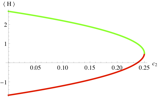
Figure 1: Expectation value of the two-level-atom Hamiltonian as a function of $c_{2}$, with $h_{0}=1$, $h_{1}=\sqrt{2}$, $h_{2}=e$, and $h_{3}=\pi$.

This procedure gives the eigenvalues and eigenvectors of the Hamiltonian and besides one gets information on the mean values associated to mixed states, as function of $c_{2}$.

3.2 Case $d=3$

We consider a particular Hamiltonian describing a two-mode Bose–Einstein condensate [28, 29],

$$\hat{H}=a\,\hat{J}_{z}+b\hat{J}_{z}^{2}+c\hat{J}_{x},$$ (17)

where $\hat{J}_{k}$ denotes the $k$-th component of the angular momentum operator. The parameter $a$ corresponds to the difference in the chemical potentials between the wells, $b$ represents the atom–atom interaction, and $c$ is related to the atom tunneling parameter.

For the qutrit case, one substitutes the three-dimensional representation of the angular momentum operators, and the generators $\hat{\lambda}_{k}$, with $k=1,2,\cdots,8$ can be realized in terms of the Gell-Mann matrices. Thus, an arbitrary density matrix is denoted by

$$\hat{\rho}=\left(\begin{array}[]{ccc}\frac{1}{3}+\frac{1}{2}\left(\lambda_{7}+\frac{1}{\sqrt{3}}\lambda_{8}\right)&\frac{1}{2}\left(\lambda_{1}-i\,\lambda_{4}\right)&\frac{1}{2}\left(\lambda_{2}-i\,\lambda_{5}\right)\\ \frac{1}{2}\left(\lambda_{1}+i\,\lambda_{4}\right)&\frac{1}{3}-\frac{1}{2}\left(\lambda_{7}-\frac{1}{\sqrt{3}}\lambda_{8}\right)&\frac{1}{2}\left(\lambda_{3}-i\,\lambda_{6}\right)\\ \frac{1}{2}\left(\lambda_{2}+i\,\lambda_{5}\right)&\frac{1}{2}\left(\lambda_{3}+i\,\lambda_{6}\right)&\frac{1}{3}-\frac{1}{\sqrt{3}}\lambda_{8}\end{array}\right)\ ,$$ (18)

and one has a similar expression for the Hamiltonian. Comparing with the $j=1$ angular momentum representation, one obtains that the parameters different from zero are

$$h_{0}=2\,b,\quad h_{1}=h_{3}=\sqrt{2}\,c,\quad h_{7}=a+b,\quad h_{8}=({3\,a-b})/{\sqrt{3}}\ .$$ (19)

Substituting the previous expressions for the density matrix and the Hamiltonian into Eq. (5), we obtain the function $f$ in the form

$$f(\lambda_{k},\Lambda_{2},\Lambda_{3},a,b,c,c_{2},c_{3})=$$

$$\qquad\frac{2}{3}b+\frac{\sqrt{2}}{2}c\left(\lambda_{1}+\lambda_{3}\right)+\frac{1}{2}\left(a+b\right)\lambda_{7}+\frac{\sqrt{3}}{6}\left(3a-b\right)\lambda_{8}+{\Lambda_{2}}\biggl{(}c_{2}-\frac{1}{3}+\frac{1}{4}\,\lambda^{2}\biggr{)}$$

$$\quad+\Lambda_{3}\biggl{(}c_{3}-\frac{1}{27}+\frac{1}{12}\lambda^{2}-\frac{1}{4}\left(\lambda_{1}\lambda_{2}\lambda_{3}+\lambda_{3}\lambda_{4}\lambda_{5}-\lambda_{2}\lambda_{4}\lambda_{6}+\lambda_{1}\lambda_{5}\lambda_{6}\right)+\frac{1}{12\sqrt{3}}\lambda_{8}^{3}$$

$$\quad-\frac{1}{8}\left(\lambda_{2}^{2}-\lambda_{3}^{2}+\lambda_{5}^{2}-\lambda_{6}^{2}\right)\lambda_{7}-\frac{1}{8\sqrt{3}}\left(2\lambda_{1}^{2}-\lambda_{2}^{2}-\lambda_{3}^{2}+2\lambda_{4}^{2}-\lambda_{5}^{2}-\lambda_{6}^{2}+2\lambda_{7}^{2}\right)\lambda_{8}\biggr{)}\ ,$$ (20)

where we define $\lambda=\sqrt{\lambda^{2}_{1}+\lambda^{2}_{2}+\lambda^{2}_{3}+\lambda^{2}_{4}+\lambda^{2}_{5}+\lambda^{2}_{6}+\lambda^{2}_{7}+\lambda^{2}_{8}}$. The extrema of the previous function with respect to $\lambda_{1},\ldots\lambda_{8},\Lambda_{2},\Lambda_{3}$, are obtained numerically by establishing different values of the set of parameters $\{a,b,c,c_{2},c_{3}\}$. Notice that the $c_{2}$ and $c_{3}$ are not independent parameters, and they are keeping track of the purity of the extremal density matrices. If we define $\tau_{2}=\tr{\rho^{2}}$ and $\tau_{3}=\tr{\rho^{3}}$, then following [30], it is straightforward to get the compatible region of the parameters $\tau_{2}$ and $\tau_{3}$. For the set $(c_{2},c_{3})=(1/3,1/27)$, one gets the extremal density matrix, $\rho^{c}=\hat{I}/3$, for the mixed state with maximum entropy and $\langle H\rangle_{c}=2\,b/3$.

To illustrate the procedure, we consider three different choices of the mentioned set of parameters. The obtained expectation values of the Hamiltonian are plotted in Fig. 2 as functions of $a$, $b$, $c$. The pure states are associated to $c_{2}=c_{3}=0$, and we find that there are $3$ extremal solutions for the parameters of the density matrix which are indicated by black continuous lines. Comparing these different mean values of the Hamiltonian with the corresponding exact diagonalizations, one finds a complete agreement with the energy spectra.

For $c_{2}$ and $c_{3}$ different from zero, additionally one gets information on the mean values of the energy. We obtain in this case that the number of mean values of mixed states is related to the symmetric group of $3$ dimensions; thus, for $c_{2}=\frac{29}{100},c_{3}=\frac{1}{50}$, there are $6$ colored continuous lines indicating the expectation values of the Hamiltonian of the possible mixed states.

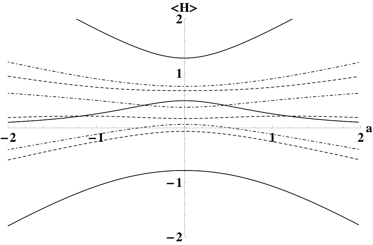
(a) $\langle\hat{H}\rangle$ as a function of the parameter $a$, with $b~{}=~{}0.5$, and $c~{}=~{}-1$.

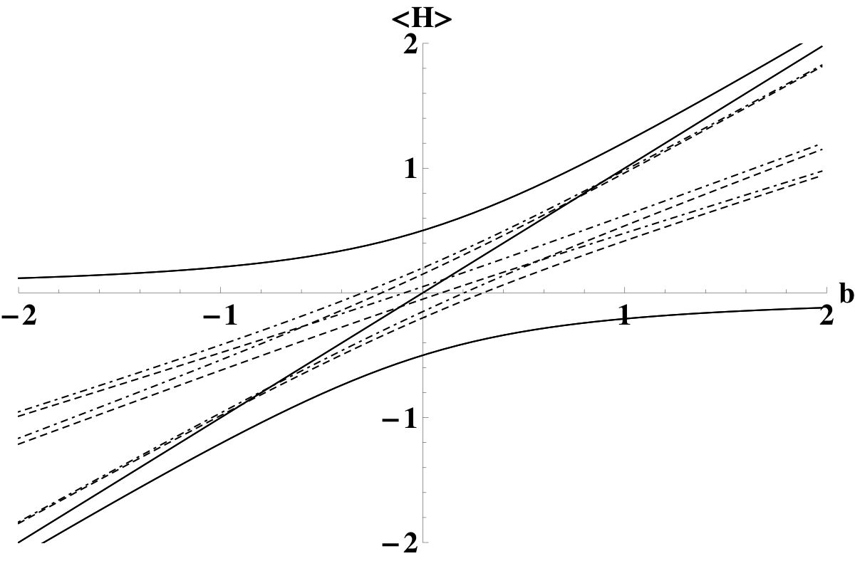
(b) $\langle\hat{H}\rangle$ as a function of the parameter $b$, with $a=0.5$, and $c=0.5$.

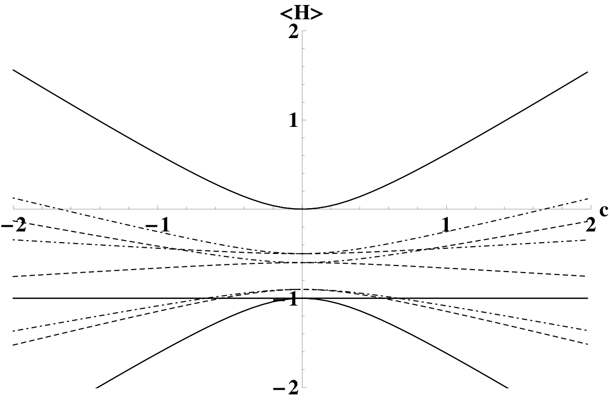
(c) $\langle\hat{H}\rangle$ as function of $c$, with $a=0.5$, $b=-1$.

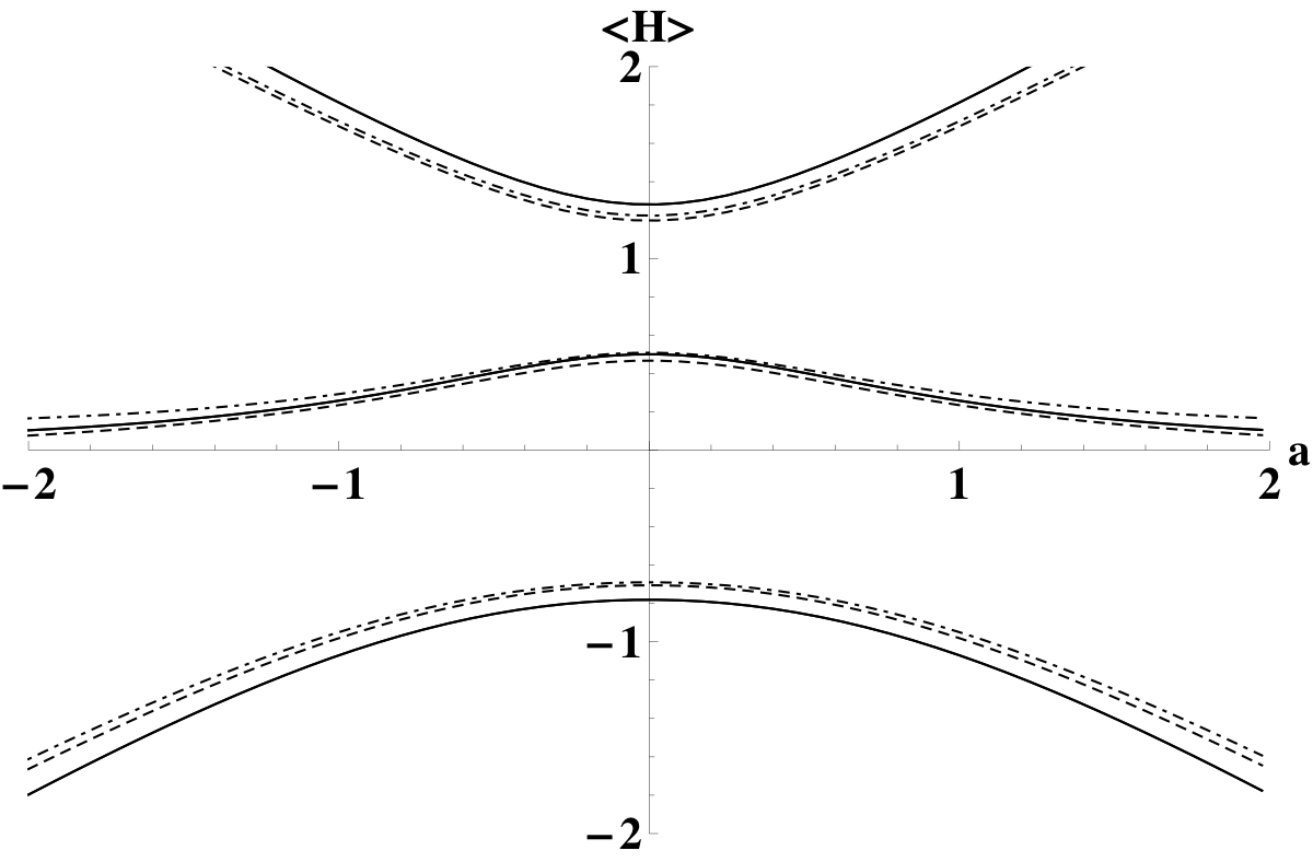
(d) $\langle\hat{H}\rangle$ as a function of $a$, with $b=-0.5$, $c=-1$.

Figure 2: Three different plots of the expectation value $\langle\hat{H}\rangle$ as a function of the parameters of the Hamiltonian for $(c_{2}=\frac{29}{100}$ and $c_{3}=\frac{1}{50})$ (a–c) and $(c_{2}=\frac{1921}{40000}$ and $c_{3}=\frac{399}{800000})$ (d) in the domain determined in [30]. They are indicated by dashed lines and dash-dotted lines; notice that there are two independent solutions, each of one with three curves. The three black curves correspond to the pure states of the system, where $c_{2}=c_{3}=0$.

4 Entropy and energy relations

It is known [24] that for two given density matrices $\rho$ and $\sigma$, the positivity condition for their relative entropy is given by

$${\rm Tr}(\rho\,{\ln}\rho-\rho\ln\sigma)\geq 0.$$ (21)

The matrices $\rho$ and $\sigma$ satisfy the properties $\rho^{\dagger}=\rho$, $\sigma^{\dagger}=\sigma$, $\rho\geq 0$, $\sigma\geq 0$ and ${\rm Tr}\,\rho={\rm Tr}\,\sigma=1$. On the other hand, two arbitrary matrices which have these properties satisfy inequality (21).

We are going to use this inequality considering the Hamiltonian matrix $H$ of a qudit system, by defining the matrix

$$\rho_{H}=\frac{e^{H}}{{\rm Tr}\,e^{H}},$$ (22)

which has the properties Tr $\rho_{H}=1$ and $\rho_{H}\geq 0$.

Let us write the positivity conditions of relative entropy of two matrices $\rho$ and $\rho_{H}$

$${\rm Tr}\left(\rho\ln\rho-\rho\ln\frac{e^{H}}{{\rm Tr}e^{H}}\right)\geq 0.$$ (23)

Using the definition of the von Neumann entropy $S$ associated with the density matrix of the state, which reads $S=-{\rm Tr}(\rho\ln\rho)$, one can rewrite inequality (23) in the form

$$S+\langle H\rangle\leq\ln\left({\rm Tr}e^{H}\right),$$ (24)

where the mean energy is given by $E=\langle H\rangle$.

For an arbitrary Hamiltonian $H$, one introduces the partition function

$$Z(\beta)={\rm Tr}\left(e^{-\beta H}\right),$$ (25)

where $T=\beta^{-1}$ is interpreted as a temperature, and the matrix $\rho(\beta)=\exp(-\beta H)/Z(\beta)$ can be interpreted as the density matrix of the system in thermal equilibrium state. It is known that the partition function $Z(\beta)$ determines all thermodynamic properties of the system (cf. [27]). Then inequality (24) can be rewritten in the form

$$E+S\leq\ln Z(\beta=-1).$$ (26)

Thus, we got for an arbitrary quantum system a bound for the sum of the mean energy value and the von Neumann entropy, and this bound is determined by the partition function evaluated in a particular value of temperature, $T=-1$.

For example, for a two-level atom in the state determined by the density matrix given in Eq. (9) with the condition $\lambda^{2}_{1}+\lambda^{2}_{2}+\lambda^{2}_{3}\leq 1$, and the Hamiltonian matrix given in Eq. (10), inequality (26) reads

$$\frac{1}{4}\,{\rm Tr}\left\{\left(\begin{array}[]{cc}1+\lambda_{3}&\lambda_{1}-i\,\lambda_{2}\\ \lambda_{1}+i\,\lambda_{2}&1-\lambda_{3}\end{array}\right)\left(\begin{array}[]{cc}h_{0}+h_{3}&h_{1}-i\,h_{2}\\ h_{1}+i\,h_{2}&h_{0}-h_{3}\end{array}\right)\right\}$$ (31)

$$-{\rm Tr}\left\{\left(\begin{array}[]{cc}\frac{1+\lambda_{3}}{2}&\frac{\lambda_{1}-i\,\lambda_{2}}{2}\\ \frac{\lambda_{1}+i\,\lambda_{2}}{2}&\frac{1-\lambda_{3}}{2}\end{array}\right)\ln\left(\begin{array}[]{cc}\frac{1+\lambda_{3}}{2}&\frac{\lambda_{1}-i\,\lambda_{2}}{2}\\ \frac{\lambda_{1}+i\,\lambda_{2}}{2}&\frac{1-\lambda_{3}}{2}\end{array}\right)\right\}\leq\ln\,{\rm Tr}\,(e^{H})\,.$$ (36)

Notice that the last expression is invariant under unitary transformations and thus one can write ${\rm Tr}(e^{H})=e^{E_{1}}+e^{E_{2}}$, where the energy levels $E_{1}$ and $E_{2}$ are the solutions of the secular equation ${\rm Det}(H-EI_{2})=0$.

For any state, one has that the inequality (31) can be written as follows

$$F=\ln Tr(e^{H})-Tr(\rho H)-S\geq 0,$$ (37)

where we define the function $F$ in terms of $(\lambda_{1},\lambda_{2},\lambda_{3})$ and $(h_{0},h_{1},h_{2},h_{3})$. By substituting the extremal parameters of the density matrix given in expression (13) the function $F$ takes the form

$$F(h,\delta)=\frac{1}{2}\left(-\delta\,h+2\,\delta\,\hbox{arctanh}{(\delta)}+2\,\ln{\left(\cosh{\frac{h}{2}}\right)}+\ln{(1-\delta^{2})}\right)\geq 0,$$ (38)

where $(h,\delta)$ were defined after Eq. (13). This function is displayed in Fig. 3 as a function of the $\delta$ and $h$. Notice that always it is larger than zero. The corresponding contour levels are also positive.

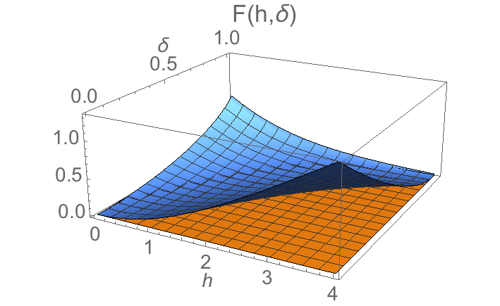
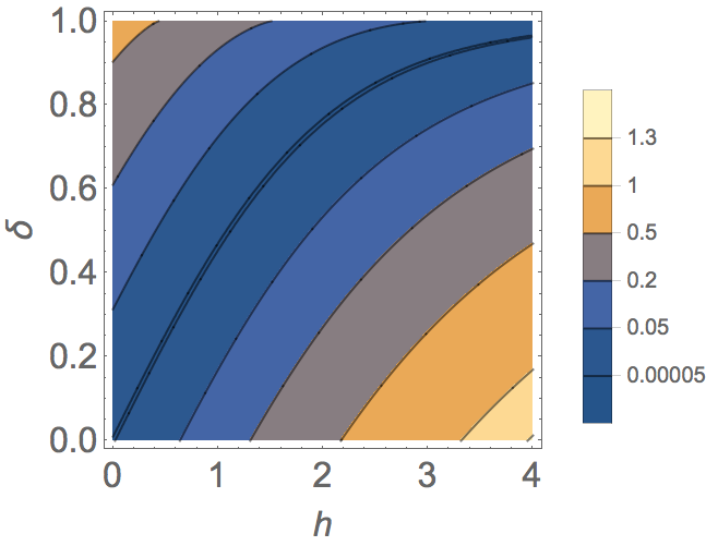
Figure 3: The entropy–energy inequality (at the top) and a contour level plot of this inequality as a function of $h$ and $\delta$ (at the bottom).

Similar inequalities can be obtained for any Hermitian operator, and the obtained result for the Pauli matrix $\sigma_{k}$ with $k=x,y,z$, can be written in the form

$$F_{\sigma_{k}}(h,\delta)=-\frac{h_{k}\,\delta}{h}+\,\delta\,\hbox{arctanh}{(\delta)}+\ln{\left(e+1/e\right)}+\,\ln{\left(\frac{1-\delta^{2}}{4}\right)}\geq 0\,,$$ (39)

with $k=x,y,z$. For $k=x$, the result is displayed in Fig. 4.

One can obtain another important inequality between the energy and the partition function by considering

$${\rm Tr}\left\{\frac{e^{H}}{{\rm Tr}(e^{H})}\ln\left(\frac{e^{H}}{{\rm Tr}(e^{H})}\right)-\frac{e^{H}}{{\rm Tr}(e^{H})}\ln\rho\right\}\geq 0,$$ (40)

which can be written for any state $\rho$ in the form

$$-\frac{\partial Z(\beta)}{\partial\beta}\Big{|}_{\beta=-1}-\,Z(\beta=-1)\,\ln Z(\beta=-1)\geq{\rm Tr}(e^{H}\ln\rho)\,.$$ (41)

Also inequality (26) is accompanied by the inequality $-E+S\leq\ln Z(\beta=1)$, which means that the partition function provides the bound for the difference of entropy and energy.

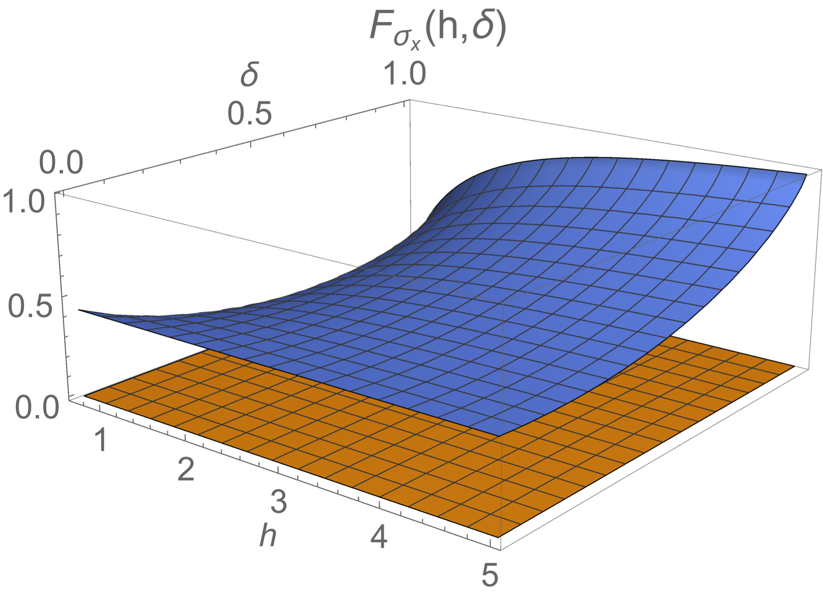
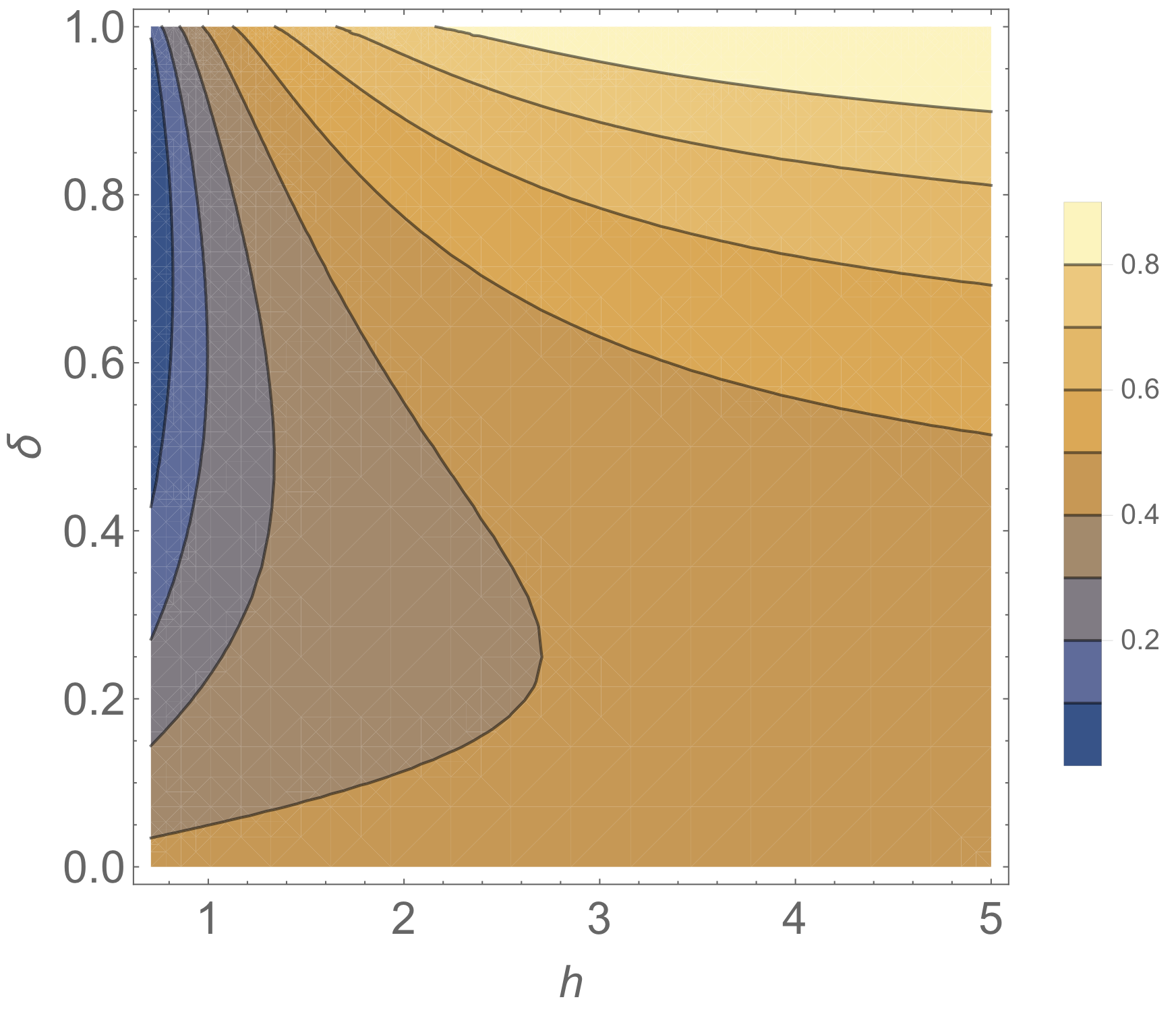
Figure 4: The entropy and $\sigma_{x}$ inequality (at the top) and a contour level plot of the inequality as a function of $h=\sqrt{\frac{1}{2}+h^{2}_{2}+h^{2}_{3}}$ and $\delta$ (at the bottom). The expectation value of $\sigma_{x}$ is evaluated with respect to one extremal density matrix of the general Hamiltonian in the two dimensions.

5 Summary and Conclusions

We suggested to study the properties of a qudit system considering the mean values of its Hamiltonian with respect to a generic density matrix, which includes the special cases of pure states. The number of parameters which determine the mean values of the Hamiltonian in this case is equal to the number of parameters determining the density matrix. Due to this, the information contained in the mean values of the Hamiltonian is sufficient to reconstruct the Hamiltonian, including both its spectrum and its eigenvectors. We demonstrated how the Hamiltonian spectrum is recovered finding all the extreme density operators which minimize the mean values of the Hamiltonian. The suggested approach for finding all the properties of the Hamiltonian has common features with quantum tomography. In the quantum tomography approach, one determines the density operator by making measures in all the reference frames of the information contained in its mean value. Therefore, the mean values are calculated for an ensemble of basis determined by sufficient number of parameters associated to unitary matrices transforming the density operator (or equivalently, changing the basis where the means are calculated). Thus, we found that the description of the Hamiltonian by the mean values approach and the description of density operators by tomographic approach have common features. We demonstrated that for $d=2$ and 3; the Hamiltonian spectrum is completely recovered using the mean value approach. We surmise on the basis of the number of parameters of the test variational density matrix that the complete recovering of the spectrum takes place for arbitrary dimensions. The previous conjecture is based in the following calculation: For pure states a test density matrix with 4 real parameters can be used and then one can get the exact energy spectrum of the system while with the extremal density matrices associated to the CS one has only approximate results for the energy levels. The problem of the convenience of our approach in comparison with standard diagonalisation of the Hamiltonian has to be clarified. We point out that our approach can be applied to arbitrary hermitian matrices, i.e., to arbitrary observables. The known properties of density matrices and von Neumann entropy were used to formulate and verify a new inequality for a qudit system between the energy and the entropy. We mapped the Hamiltonian matrix onto a density-like nonnegative matrix, and applied the property of nonnegativity of relative entropy connecting two density matrices. The obtained result for the sum (difference) of entropies and mean value of the Hamiltonian is that this sum (difference) is bound. The bound is determined by the partition function evaluated at a specific value of its argument. We verified the new inequality on an example of a qubit system. The obtained result is valid for all the states, including entangled states of multi-qudit systems. One can get analogous inequalities for other hermitian operators corresponding to physical observables. We will study this aspect of the inequalities in future publications.

6 Acknowledgements

This work was partially supported by CONACyT-México and PAPIIT-UNAM (IN110114).

References

References

- [1] López-Moreno E and Castaños O, 1996 Phys. Rev. C 54 2374.
- [2] Castaños O, López-Peña R, Hirsch J G, and López-Moreno E, 2005 Phys. Rev. B 72 012406.
- [3] Castaños O, Nahmad-Achar E, López-Peña R, and Hirsch J G, 2011 Phys. Rev. A 83 051601.
-
[4]
Cordero S, Castaños O, López-Peña R, and Nahmad-Achar E,
2013 J. Phys. A: Math. Theor. 46 505302. - [5] Gilmore R 1979 J. Math. Phys. 20 891.
- [6] Gilmore R 1981 Catastrophe Theory for scientists and engineers Wiley (New York).
- [7] Bertrand J and Bertrand D, 1987 Found. Phys. 17 397.
- [8] Vogel K and Risken H, 1989 Phys. Rev. A 40 2847.
- [9] Mancini S, Man’ko V I, and Tombesi P, 1996 Phys. Lett A 213 1.
- [10] Ibort A, Man’ko V I, Marmo G, Simoni A, and Ventriglia F, 2009 Phys. Scr. 79 065013.
-
[11]
Castaños O, López-Peña R, Man’ko M A, and Man’ko V I ,
2004 Phys. A: Math. Gen. 37 8529. - [12] Dodonov V V and Man’ko V I, 1997 Phys. Lett. A 229 335.
- [13] Man’ko V I and Man’ko O V, 1997 J. Exp. Theor. Phys. 85 430.
- [14] Castaños O, López-Peña R, Man’ko M A, and Man’ko V I, 2003, J. Phys. A: Mat. Gen. 36 4677.
- [15] Castaños O, López-Peña R, Man’ko M A, and Man’ko V I, 2003, J. J. Opt. B: Semiclass. Opt. 5 227.
- [16] Landau L D, 1927 Z. Physik 45 430.
- [17] von Neumann J, 1932 Mathematische Grundlagen der Quantenmechanik, Springer Berlin.
- [18] Tilma T and Sudarshan E C G, 2002 J. Phys A: Math. Gen. 3510467.
- [19] Kimura G, 2003 Phys. Lett. A 314 339.
- [20] Byrd M S and Khaneja N, 2003 Phys. Rev. A 68 062322.
- [21] Jarlskog C, 2006 J. Math. Phys. 47 013507.
- [22] Brüning E, Mäkelä H, Messina A, and Petruccione F, 2012 J. Mod. Opt. 59 1.
- [23] Akhtarshenas S J, 2006 Opt. Spectrosc. 103 411.
-
[24]
Nielsen M A, and Chuang I L, 2010 Quantum Computation and Quantum Information ,
Cambridge University Press. - [25] Chernega V N, Man’ko O V, and Man’ko V I, 2014 J. Russ. Laser Res. 35 278
- [26] Man’ko M A, and Man’ko V I, 2014 Phys. Scr. T160 014030.
-
[27]
Kubo R, 1965 Statistical Mechanics: An Advanced Course with Problems and Solutions,
Elsevier Science. - [28] Milburn G J, Corney J, Wright E W, and Walls D F, 1997 Phys. Rev. Lett. A 55 4318.
-
[29]
Pérez-Campos C, González-Alonso J R, Castaños O, and López-Peña R,
2010 Ann. Phys. (N.Y.) 325 325. - [30] Gerdt V P, Khvedlidze A M, and Palii Yu G, 2014 J. Math. Sci. 200 682.