Strong-coupling ansatz for the one-dimensional Fermi gas in a harmonic potential

Abstract

A major challenge in modern physics is to accurately describe strongly interacting quantum many-body systems. One-dimensional systems provide fundamental insights since they are often amenable to exact methods. However, no exact solution is known for the experimentally relevant case of external confinement. Here, we propose a powerful ansatz for the one-dimensional Fermi gas in a harmonic potential near the limit of infinite short-range repulsion. For the case of a single impurity in a Fermi sea, we show that our ansatz is indistinguishable from numerically exact results in both the few- and many-body limits. We furthermore derive an effective Heisenberg spin-chain model corresponding to our ansatz, valid for any spin-mixture, within which we obtain the impurity eigenstates analytically. In particular, the classical Pascal’s triangle emerges in the expression for the ground-state wavefunction. As well as providing an important benchmark for strongly correlated physics, our results are relevant for emerging quantum technologies, where a precise knowledge of one-dimensional quantum states is paramount.

One-dimensional systems occupy a unique place in strongly correlated many-body physics, as many are exactly solvable via methods such as the Bethe Ansatz. Likewise, the exactly solvable harmonic oscillator plays a central role in quantum mechanics. However, when one combines these two fundamental models and considers interacting fermions in a 1D harmonic potential, there is no known solution in general Guan et al. (2013). While the problem may be solved analytically for 2 particles Busch et al. (1998), and numerically up to $\sim$10 particles Gharashi and Blume (2013); Volosniev et al. (2014); Deuretzbacher et al. (2014); Bugnion and Conduit (2013); Sowiński et al. (2013); Astrakharchik and Brouzos (2013), the calculation rapidly becomes untenable beyond that. Recent theoretical works have proposed analytic forms of the lowest energy wavefunctions near the Tonks-Girardeau (TG) limit of infinitely strong contact interactions Guan et al. (2009); Girardeau (2010); Cui and Ho (2014), but these do not match exact numerical studies Gharashi and Blume (2013); Volosniev et al. (2014); Deuretzbacher et al. (2014) once the particle number exceeds three. Here, we present a novel, highly accurate ansatz for the wavefunction of the two-component 1D Fermi gas in a harmonic potential with strong repulsive interactions.

Harmonically confined 1D systems have received a considerable amount of interest, particularly since the experimental realization in ultracold atomic Bose Paredes et al. (2004); Kinoshita et al. (2004) and Fermi gases Serwane et al. (2011); Zürn et al. (2012); Wenz et al. (2013); Zürn et al. (2013); Murmann et al. (2015). Experimentalists have trapped fermionic ⁶Li atoms in a 1D waveguide, with a high degree of control over both the number of particles in two hyperfine states and the interspecies interaction strength. This allows one to study the evolution from few to many particles, as well as the possibility of magnetic transitions as the interactions are tuned through the TG limit. The approach we propose here provides a way to tackle the regime near the TG limit, which has been investigated in a recent experiment Zürn et al. (2012). In this case, the ground-state manifold in the confined system consists of ${{N_{\uparrow}+N_{\downarrow}}\choose{N_{\downarrow}}}$ nearly degenerate states, where $N_{\uparrow}$ ($N_{\downarrow}$) is the number of spin-$\uparrow$ (spin-$\downarrow$) particles. For the “impurity” problem consisting of a single $\downarrow$ particle ($N_{\downarrow}=1$) in a sea of $N_{\uparrow}$ majority particles, we generate all these states in an essentially combinatorial manner. We show that the overlap between our ansatz wavefunction and exact states obtained by numerical calculations exceeds 0.9997 for $N_{\uparrow}\leq 8$. In particular, the overlap with the exact ground state for large repulsive interactions is found to extrapolate to a value $\sim 0.9999$ as $N_{\uparrow}\to\infty$. This remarkable accuracy shows that our ansatz effectively solves the strongly interacting single $\downarrow$ problem in a harmonic potential, from the few- to the many-body limit.

We have furthermore mapped the strongly interacting 1D problem onto an effective Heisenberg spin chain of finite length Matveev (2004); Matveev and Furusaki (2008); Deuretzbacher et al. (2014), and we derive an analytical expression for the Hamiltonian within which our ansatz is exact. In this case, our ansatz for the impurity wavefunctions in the spin basis corresponds to discrete Chebyshev polynomials. In accordance with the orthogonality catastrophe Anderson (1967), we find that the overlap with the non-interacting many-body ground state (i.e., the quasiparticle residue) tends to zero in the thermodynamic limit $N_{\uparrow}\to\infty$. However, surprisingly, in this limit the ground-state probability distribution of the impurity is a Gaussian only slightly broadened compared with the non-interacting ground state. As we argue, our effective spin model is expected to accurately describe any $N_{\downarrow}$, $N_{\uparrow}$, opening up the possibility of addressing the strongly interacting 1D Fermi gas with powerful numerical methods for lattice systems. We also discuss how our results can be extended to higher excited states and how they may be probed in cold-atom experiments. Our findings are of fundamental relevance for emerging quantum technologies where an accurate knowledge of 1D quantum states is needed, such as for engineering efficient state transfer Christandl et al. (2004), and for understanding relaxation and thermalisation in out-of-equilibrium quantum systems Eisert et al. (2015).

Results

The model.

We consider $N_{\uparrow}$ fermions in spin state $\uparrow$ and $N_{\downarrow}$ fermions in spin state $\downarrow$, both with mass $m$, confined in a 1D harmonic potential. The total number of particles is written as $N_{\uparrow}+N_{\downarrow}=N+1$, which is convenient when we consider the impurity problem below. The Hamiltonian is thus

$${\cal H}=\sum_{i=0}^{N}\left[-\frac{\hbar^{2}}{2m}\frac{\partial^{2}}{\partial x_{i}^{2}}+\frac{1}{2}m\omega^{2}x_{i}^{2}\right]+g\sum_{i<j}\delta(x_{i}-x_{j}),$$ (1)

where the coupling $g$ quantifies the strength of the short-range interactions and $\omega$ is the harmonic oscillator frequency. Note that particles with the same spin do not interact since their wavefunction vanishes when $|x_{i}-x_{j}|\to 0$ due to antisymmetry under particle exchange. Since ${\cal H}$ commutes with the total spin operator, the eigenstates have well defined spin projection $S_{z}=(N_{\uparrow}-N_{\downarrow})/2$ and total spin $S$. In the following, we use harmonic oscillator units where $\omega=m=\hbar=1$.

In the TG limit, the coupling strength $g\to\infty$ and the system simplifies significantly due to the form of the boundary conditions when two particles approach each other. Specifically, for a given wavefunction $\psi({\bf x})$, the infinite repulsion requires $\lim_{x_{ij}\to 0}\psi({\bf x})=0$, with $x_{ij}\equiv x_{i}-x_{j}$ the relative coordinate for any pair of fermions with opposite spin, and ${\bf x}=(x_{0},x_{1},\dots,x_{N})$. Identical fermions always obey this condition, as mentioned above. Since all particles experience the same boundary conditions, the ground-state manifold for a system with fixed $S_{z}$ contains ${N_{\uparrow}+N_{\downarrow}}\choose{N_{\downarrow}}$ degenerate states, corresponding to the number of unique configurations of $\uparrow$ and $\downarrow$ particles.

The simplest eigenstate of the Hamiltonian (1) is the fully ferromagnetic state, corresponding to the maximum total spin $S=(N+1)/2$. In this case, the spin part of the wavefunction is always symmetric, regardless of $S_{z}$, and thus the wavefunction in real space must be antisymmetric. Specifically, the wavefunction takes the form of a Slater determinant of single-particle harmonic oscillator wavefunctions, and can be written Girardeau et al. (2001)

$$\psi_{0}({\bf x}) ={\cal N}_{N}\left(\prod_{0\leq i<j\leq N}x_{ij}\right)e^{-\sum_{k=0}^{N}x_{k}^{2}/2},$$ (2)

with normalization

$${\cal N}_{N}=\frac{1}{\sqrt{(N+1)!}}\sqrt{\frac{2^{\frac{1}{2}N(N+1)}}{\pi^{\frac{1}{2}(N+1)}\prod_{n=0}^{N}n!}}\ .$$

The ferromagnetic state corresponds to that of $N+1$ identical fermions, and thus its energy is $E_{0}=\sum_{n=0}^{N}(n+1/2)-1/2=N(N+2)/2$, where we subtract the center-of-mass zero point energy. Furthermore, it is an eigenstate for all $g$ since the wavefunction antisymmetry guarantees that it vanishes when $x_{ij}\to 0$ so that it does not experience the particle-particle interaction.

For a given $S_{z}$ (corresponding to fixed $N_{\uparrow}$ and $N_{\downarrow}$), the remaining eigenstates with the same energy $E_{0}$ in the TG limit may be characterized by other values of $S$. For instance, for $N_{\uparrow}=N_{\downarrow}=1$, there are two states, characterized by either $S=0$ or $S=1$. However, for general particle number, spin alone is not sufficient to determine the states with $S<(N+1)/2$, since the degeneracy of the ground-state manifold is ${N_{\uparrow}+N_{\downarrow}}\choose{N_{\downarrow}}$ whereas the number of different $S$ for a given $S_{z}$ is $1+{\rm min}(N_{\uparrow},N_{\downarrow})$. Thus, in order to construct a unique orthogonal basis of eigenstates in the TG limit, we must consider how the states in the ground-state manifold evolve as $g\to\infty$, as illustrated in Fig. 1. We mostly focus on the impurity problem where we have one $\downarrow$ particle at position $x_{0}$ and $N$ $\uparrow$ particles at positions $x_{i}$ with $1\leq i\leq N$. In this case, we have $N$ eigenstates with spin $S=S_{z}=(N-1)/2$, in addition to the ferromagnetic state.

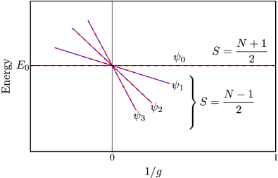
Figure 1: Energy levels in the Tonks-Girardeau limit. We display the exact energies $\langle\psi_{l}|{\cal H}|\psi_{l}\rangle$ (red) and the result of our ansatz $\left<\tilde{\psi}_{l}\right|{\cal H}\left|\tilde{\psi}_{l}\right>$ (blue dashed), given by $E_{0}-{\mathcal{C}}_{l}/g$ in this limit, for the case of one $\downarrow$ particle and $N=3$ $\uparrow$ particles. For $g<0$, there is also a two-body bound state at negative energies which we do not show.

Ground-state manifold in the TG limit.

To construct the wavefunctions for the impurity problem with $S=S_{z}=\frac{N-1}{2}$, it is useful to define a complete (but not orthogonal) set of basis functions involving $\phi_{0}=\psi_{0}({\bf x})$ and the $N$ states:

$$\phi_{l} =\psi_{0}({\bf x})\sum_{1\leq i_{1}<\cdots<i_{l}\leq N}s_{i_{1}}\cdots s_{i_{l}},\hskip 14.22636pt1\leq l\leq N,$$ (3)

where $s_{i}\equiv\mbox{sign}(x_{i0})$. For simplicity, we omit the dependence of $\phi_{l}$ on the coordinates. Each sign function simply replaces a zero-crossing in the Slater determinant (2) with a cusp at the position where the impurity meets a majority ($\uparrow$) particle ($x_{i0}=0$). As an example, for $N=2$ we have basis functions:

$$\phi_{0}= \ {\cal N}_{2}\ x_{12}x_{01}x_{02}\ e^{-\left(x_{0}^{2}+x_{1}^{2}+x_{2}^{2}\right)/2},$$

$$\phi_{1}= \ {\cal N}_{2}\ x_{12}\left(|x_{01}|x_{02}+x_{01}|x_{02}|\right)\ e^{-\left(x_{0}^{2}+x_{1}^{2}+x_{2}^{2}\right)/2},$$

$$\phi_{2}= \ {\cal N}_{2}\ x_{12}|x_{01}x_{02}|\ e^{-\left(x_{0}^{2}+x_{1}^{2}+x_{2}^{2}\right)/2}.$$

The basis functions are clearly degenerate with the ferromagnetic state (2) when $g\rightarrow\infty$, since the interaction energy vanishes while the energy of motion in the harmonic potential is the same for all $\phi_{l}$. This can be shown by noting that for any ordering of the particles (say $x_{0}<x_{1}<...<x_{N}$) we have $\phi_{l}\propto\psi_{0}({\bf x})$. Thus all eigenstates of the ground state manifold in the TG limit must be linear combinations of the basis functions. Note that alternatively we could have chosen a basis set whose functions are non-zero only for a particular ordering of particles as in Ref. Deuretzbacher et al. (2008).

The central question we address here concerns the nature of the eigenstates in the vicinity of the TG limit, i.e., we wish to know the wavefunctions and energies perturbatively in the small parameter $1/g$. This allows one to uniquely define the eigenstates at $g\rightarrow\infty$ as being those that are adiabatically connected to the states at finite $g$. Before proceeding with degenerate perturbation theory, it is instructive to consider the structure of the exact eigenstates $\psi_{l}$ (up to corrections of order $1/g$) for $N=1$ Busch et al. (1998) and $N=2$ Guan et al. (2009),

$$N=1:\hskip 8.53581pt \psi_{0}=\phi_{0},\hskip 5.69054pt\psi_{1}=\phi_{1},$$

$$N=2:\hskip 8.53581pt \psi_{0}=\phi_{0},\hskip 5.69054pt\psi_{1}=\sqrt{\frac{3}{8}}\phi_{1},\hskip 5.69054pt\psi_{2}=\sqrt{\frac{1}{8}}(\phi_{0}-3\phi_{2}).$$ (4)

The subscripts on the wavefunctions order these in terms of decreasing energy for small but positive $1/g$. Note that the eigenstates split into two orthogonal sets which are even or odd with respect to parity, since the Hamiltonian commutes with the parity operator. Referring to Fig. 1 and focussing on the repulsive case $g>0$, we see that the ferromagnetic state $\psi_{0}$ has the maximum energy within the manifold Cui and Ho (2014), while the ground state $\psi_{N}$ has the lowest total spin, i.e., $S=S_{z}$, in accordance with the Lieb-Mattis theorem Lieb and Mattis (1962). Physically, the cusps in the wavefunction for $g\rightarrow\infty$ can easily be shifted from zero, which decreases the kinetic energy and thus leads to a lower energy compared with the ferromagnetic state. Indeed we see two patterns emerging: $\psi_{1}$ contains only states with one cusp, and only the ground state $\psi_{N}$ contains the state with the maximal number of cusps. These observations suggest that the system may lower its energy by successively acquiring more cusps in the wavefunction.

Inspired by the above considerations, we now propose the following strong-coupling ansatz for the impurity eigenstates of the ground-state manifold in the vicinity of the TG limit:

• For any $N$, the exact wavefunction $\psi_{l}$ essentially corresponds to $\tilde{\psi}_{l}$, a superposition of the basis functions $\phi_{k}$ restricted to $k\leq l$.

In other words, the wavefunctions are obtained by a Gram-Schmidt orthogonalization scheme on the set of basis functions $\{\phi_{k}\}$: $\tilde{\psi}_{1}$ is obtained by adding one cusp to $\psi_{0}$, $\tilde{\psi}_{2}$ is obtained by adding one more cusp and then orthogonalising it to $\tilde{\psi}_{0}$, and so on. We emphasize that the ansatz allows one to obtain the entire ground-state manifold using linear algebra manipulations only. Thus, one can go far beyond the limit $N\lesssim 9$ of current state of the art calculations Volosniev et al. (2014). In fact, we will see that the ansatz allows us to obtain analytic expressions for all wavefunctions in the ground-state manifold for any $N$. We will show that the ansatz is remarkably accurate compared with exact numerical results, and that it allows one to calculate several observables analytically, even in the many-body limit.

The procedure for constructing our ansatz wavefunctions $\tilde{\psi}$ as outlined above can in fact be performed straightforwardly even for large $N$, by noting that the inner products of the basis functions (3), $\Phi_{ln}\equiv\langle\phi_{l}|\phi_{n}\rangle$, may be calculated combinatorially (see Methods).

Perturbation theory around the TG limit.

To demonstrate the accuracy of our ansatz, we now turn to the explicit solution of the Schrödinger equation in the vicinity of the TG limit. Since here there are $N+1$ degenerate states, we apply degenerate perturbation theory and obtain the ground-state manifold by means of finite-matrix diagonalization, in a similar manner to Refs. Deuretzbacher et al. (2014); Volosniev et al. (2014). The energy can be written as $E\simeq E_{0}-\mathcal{C}/g$, where $\mathcal{C}$ is the 1D contact density Olshanii and Dunjko (2003); Tan (2008); Barth and Zwerger (2011). From the Hellmann-Feynman theorem, we then obtain

$$\mathcal{C}=-\left.\frac{dE}{d(g^{-1})}\right|_{g\to\infty}=-\left.\left<\frac{\partial{\cal H}}{\partial(g^{-1})}\right>\right|_{g\to\infty}\equiv\frac{\langle\left.{\Psi}\right|{\cal H}^{\prime}\left|{\Psi}\right>}{\left<\Psi|\Psi\right>},$$

which defines the perturbation ${\cal H}^{\prime}$ due to a non-zero $1/g$. The state $|\Psi\rangle$ is a linear combination of the basis states $\{\phi_{l}\}$ of the ground-state manifold: $\left|{\Psi}\right>=\sum_{n}\alpha_{n}\left|{\phi_{n}}\right>$. To obtain the eigenstates, we require $\left|{\Psi}\right>$ to be a stationary state, i.e. $\frac{\delta\mathcal{C}}{\delta\alpha_{l}^{*}}=0$, resulting in the matrix equation $\Phi^{-1}{\cal H}^{\prime}\alpha=\mathcal{C}\alpha$, with ${\mathcal{C}}$ the eigenvalue (contact density) of the state $|\Psi\rangle$. The matrix elements of ${\cal H}^{\prime}$ are

$${\cal H}^{\prime}_{ln} =\sum_{i=1}^{N}\int d{\bf x}\ \delta(x_{i0})\left.\frac{\partial\phi_{l}}{\partial x_{i0}}\right|^{x_{i0}=0^{+}}_{x_{i0}=0^{-}}\left.\frac{\partial\phi_{n}}{\partial x_{i0}}\right|^{x_{i0}=0^{+}}_{x_{i0}=0^{-}},$$ (5)

(see Methods).

For $N=1$ ($N=2$) the evaluation of ${\cal H^{\prime}}$ is straightforward and yields ${\cal H^{\prime}}_{11}=2\sqrt{2/\pi}$ (${\cal H}^{\prime}_{11}={\cal H}^{\prime}_{22}=9/\sqrt{2\pi}$), while all other elements vanish. Thus we find

$$N=1: \hskip 14.22636pt\left(\begin{array}[]{c}{\cal C}_{0}\\ {\cal C}_{1}\end{array}\right)=\sqrt{\frac{8}{\pi}}\left(\begin{array}[]{c}0\\ 1\end{array}\right),$$ (10)

$$N=2: \hskip 14.22636pt\left(\begin{array}[]{c}{\cal C}_{0}\\ {\cal C}_{1}\\ {\cal C}_{2}\end{array}\right)=\frac{27}{8\sqrt{2\pi}}\left(\begin{array}[]{c}0\\ 1\\ 3\end{array}\right),$$ (17)

where ${\cal C}_{l}\equiv\langle\psi_{l}|{\cal H}^{\prime}|\psi_{l}\rangle$ is the contact coefficient corresponding to the state $\psi_{l}$. All the eigenstates for $N\leq 2$ are in fact uniquely determined by the two symmetries of parity and spin, so that the ratios of ${\cal C}_{l}$ and the general structure of the wavefunctions in Eq. (4) hold for any confining potential that preserves parity and spin. However, these symmetries alone are not sufficient to determine the eigenstates for $N>2$, and therefore $N=3$ will provide a non-trivial test of our ansatz. In this case, the coefficients of ${\cal H}^{\prime}$ and the eigenstates may still be evaluated analytically, but their form is sufficiently complicated that we relegate these to the Methods. Converting long analytical expressions into numerical values for brevity, we obtain

$$N=3:\hskip 14.22636pt \psi_{0}=\phi_{0},$$

$$\psi_{1}=\sqrt{\frac{1}{5}}(1.00188\phi_{1}-0.00941\phi_{3}),$$

$$\psi_{2}=\frac{1}{2}(\phi_{0}-\phi_{2}),$$

$$\psi_{3}=\sqrt{\frac{1}{20}}(0.99246\phi_{1}-4.99996\phi_{3}).$$ (18)

while the contact coefficients are

$$N=3: \hskip 14.22636pt\left(\begin{array}[]{c}{\cal C}_{0}\\ {\cal C}_{1}\\ {\cal C}_{2}\\ {\cal C}_{3}\end{array}\right)=1.18067\left(\begin{array}[]{c}0\\ 1.00305\\ 3.02818\\ 6\end{array}\right).$$ (27)

These contact coefficients determine the energy splitting shown in Fig. 1 and they agree with those obtained in Ref. Deuretzbacher et al. (2014). For $N\geq 4$ we resort to a numerical evaluation of the matrix elements of ${\cal H}^{\prime}$ which may be calculated efficiently using a novel method outlined in the Methods.

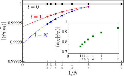
Figure 2: Accuracy of the ansatz. Overlaps between our ansatz $\tilde{\psi}_{l}$ and the exact wavefunctions $\psi_{l}$ for majority particle numbers $N\leq 8$. For the ferromagnetic state, this always equals 1 (black line). The red and blue dots depict the overlap for $\tilde{\psi}_{1}$ and $\tilde{\psi}_{N}$ (ground state) respectively. These are both 1 for $N=2$, as these states are uniquely determined by spin and parity, while they are both 0.999993 for $N=3$. The extrapolations (dashed lines) are least-squares fits of the data points to cubic polynomials. Inset: The wavefunction overlap of Girardeau’s proposed state Girardeau (2010) with the exact ground state.

Our ansatz, however, is far simpler than the brute-force approach above. While the evaluation of the multi-dimensional integral in Eq. (5) quickly becomes untenable as $N$ increases above $\sim 10$, the implementation of our ansatz is a basic exercise in linear algebra: Applying our Gram-Schmidt orthogonalization scheme, we find the states

$$N=3:\hskip 14.22636pt \tilde{\psi}_{0}=\phi_{0},\hskip 5.69054pt\tilde{\psi}_{1}=\sqrt{\frac{1}{5}}\phi_{1},\hskip 5.69054pt\tilde{\psi}_{2}=\frac{1}{2}(\phi_{0}-\phi_{2}),$$

$$\tilde{\psi}_{3}=\sqrt{\frac{1}{20}}(\phi_{1}-5\phi_{3}).$$ (28)

Comparing Eq. (28) with Eq. (18), we see that our ansatz is extremely accurate, with only a minute deviation from the exact result for $\tilde{\psi}_{1}$ and $\tilde{\psi}_{3}$ ($\psi_{0}$ and $\psi_{2}$ are determined exactly from parity and spin). We note that our proposed wavefunctions are identical to those obtained numerically in Ref. Gharashi and Blume (2013), illustrating that the results of our ansatz are essentially indistinguishable from numerical calculations.

We now demonstrate explicitly that the very high accuracy of our ansatz holds also for higher particle number $N$, and that it even seems to hold in the many-body limit. A natural measure of its accuracy is the wavefunction overlap $|\langle\left.{\psi_{l}}\right|\tilde{\psi}_{l}\rangle|$ between the exact eigenstates $\psi_{l}$ and our proposed ones $\tilde{\psi}_{l}$. Writing the wavefunctions as $\psi_{l}=\sum_{n=0}^{N}L_{ln}\phi_{n}$ and $\tilde{\psi}_{l}=\sum_{n=0}^{N}\tilde{L}_{ln}\phi_{n}$, the overlap is simply $|(\tilde{L}\Phi L^{T})_{ll}|$. For the two non-exact states with $N=3$ discussed above, we then find this quantity to be 0.999993, where we remind the reader that this is the numerical value of an analytic result (see Methods). Strikingly, we find that the overlap exceeds $0.9997$ for all states up to $N=8$, with the error being largest for the states “intermediate” between the ferromagnetic state $\psi_{0}$ and the ground state $\psi_{N}$. In Fig. 2, we illustrate how the wavefunction overlaps for the $\tilde{\psi}_{1}$ and $\tilde{\psi}_{N}$ always exceed 0.99994. In addition, the overlap in the ground state appears to extrapolate to a value $\sim 0.9999$ as $N\to\infty$. Our ansatz is therefore essentially indistinguishable from “numerically exact” methods, even in the many-body limit. This shows that our ansatz effectively solves the strongly interacting 1D impurity problem for general $N$.

Of particular interest is the state $\psi_{N}$, the ground state for repulsive interactions. Girardeau proposed Girardeau (2010) that this state is simply given by the state with the maximum number of cusps inserted, i.e., $\psi_{\rm\tiny G}=\phi_{N}$. As shown in the inset of Fig. 2, the overlap of Girardeau’s proposed state with the exact ground state is $76\%$ for $N=8$, and it most likely tends to zero as $N\to\infty$. Thus, our ansatz is a significant improvement compared to previous proposals for the ground-state wavefunction.

We now turn to the contact coefficients of the $N+1$ energy levels in the ground-state manifold, i.e., the splitting of the spectrum at finite coupling. In Fig. 3 we show how the energy takes the following approximate form

$$E_{l}\simeq E_{0}-\frac{{\cal C}_{N}}{g}\frac{l(l+1)}{N(N+1)}.$$ (29)

Comparing with Eqs. (10), (17) and (27), we see that this expression is exact for $N=1$ and $2$, while it holds to within $3.0\%$ for $N\leq 8$. We show in the next section that the spectrum given by Eq. (29) is intimately linked with an effective Heisenberg spin Hamiltonian within which our ansatz is exact.

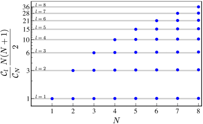
Figure 3: Contact coefficients of the ground state manifold. The contact coefficients (blue dots) of the exact eigenstates $\psi_{l}$ in the Tonks-Girardeau regime, controlling the splitting of the energy levels at finite but large coupling. The gray lines represent the approximate relationship $\frac{{\cal C}_{l}}{{\cal C}_{N}}=\frac{l(l+1)}{N(N+1)}$, see Eq. (29).

Effective Heisenberg spin chain.

We now discuss how the 1D problem can be mapped onto a Heisenberg spin model Matveev (2004); Matveev and Furusaki (2008); Deuretzbacher et al. (2014). This enables us to determine the states $\tilde{\psi}_{l}$ analytically, and it also allows us to generalise our ansatz for the impurity problem to any $N_{\downarrow}$.

In the limit $g\to\infty$, the system consists of impenetrable particles since the wavefunction must vanish when two particles approach each other. Thus, if the particles are placed in a particular order, they should retain that ordering as long as the repulsion is infinite. This allows us to consider the system in the TG limit as a discrete lattice of finite length $N+1$, where the particle furthest to the left is at site $i=0$, the next particle is at site $i=1$ and so on. A small but finite value of $1/g$ then allows neighboring particles to exchange position, introducing a nearest-neighbor spin interaction in the lattice picture. We can thus write the Hamiltonian in the lattice as

$${\cal H}\simeq E_{0}-\frac{{\cal H}^{\prime}}{g}=E_{0}+\frac{{\cal C}_{N}}{g}\sum_{i=0}^{N-1}\left[J_{i}\hat{\bf S}^{i}\cdot\hat{\bf S}^{i+1}-\frac{1}{4}J_{i}\right],$$ (30)

where $\hat{\bf S}^{i}$ is the spin operator at site $i$ and $J_{i}$ is the nearest neighbor exchange constant, which can in general depend on $i$ Volosniev et al. (2014, 2015). Subtracting the constant in each term of the sum ensures that the ferromagnetic state has energy $E_{0}$. The Hamiltonian (30) is valid to linear order in $1/g$ and the general form holds for any external potential.

The couplings $J_{i}$ in the Heisenberg model (30) can be determined by considering the single $\downarrow$ impurity problem in a new basis of position states $\left|{\downarrow_{i}}\right>$ with $0\leq i\leq N$. The lattice position $i$ corresponds to the position of the impurity relative to the $N$ majority particles. The position states are orthonormal, $\langle\left.{\downarrow_{i}}\right|\left.\downarrow_{j}\right>=\delta_{ij}$, and can be related back to $\phi_{l}$ (see Methods). The perturbation ${\cal H}^{\prime}$ may then be evaluated in the position basis of the impurity by inserting a complete set of eigenstates, yielding

$$\langle\left.{\downarrow_{i}}\right|{\cal H}^{\prime}\left|{\downarrow_{j}}\right>=\sum_{l=0}^{N}\langle\left.{\downarrow_{i}}\right|\psi_{l}\rangle\,\mathcal{C}_{l}\,\langle\psi_{l}\left|{\downarrow_{j}}\right>.$$ (31)

The matrix elements (31) provide an explicit construction of the Heisenberg Hamiltonian (30).

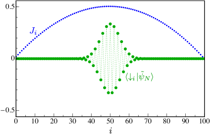
Figure 4: Exchange constants and ground state of the Heisenberg model. Illustration of the nearest-neighbor exchange constants (32) of the spin Hamiltonian (30) for $N=100$. We also show the ground-state wavefunction (48) within our ansatz (green dots).

We now determine the Heisenberg Hamiltonian within which our strong-coupling ansatz for the eigenstates is exact. Proceeding via “reverse engineering”, we form the effective Hamiltonian by replacing $\psi_{l}$ with our ansatz wavefunctions $\tilde{\psi}_{l}$ in Eq. (31). By inspection of the effective Hamiltonian for all $N\leq 100$, we find that we must use the approximation ${\cal C}_{l}\simeq{\cal C}_{N}\frac{l(l+1)}{N(N+1)}$ from Eq. (29) in Eq. (31) in order to obtain a Hamiltonian restricted to nearest-neighbor interactions, and we obtain the couplings

$$J_{i} =\frac{-\left(i-\frac{N-1}{2}\right)^{2}+\frac{1}{4}(N+1)^{2}}{N(N+1)/2}.$$ (32)

The exchange constant takes the form of an inverted parabola and is thus reminiscent of the real space harmonic oscillator potential (see Fig. 4). The form of the coefficients means that the impurity at small positive $1/g$ may minimize its energy by occupying primarily the center of the spin chain, while alternating the sign of the wavefunction on the different sites. Contrast this with the ferromagnetic state, which is a completely symmetric function of the impurity position $\left|{\psi_{0}}\right>=\frac{1}{\sqrt{N+1}}\sum_{i=0}^{N}\left|{\downarrow_{i}}\right>$. This is equivalent to the state obtained by applying the total spin lowering operator $\hat{S}_{-}=\sum_{i}\hat{S}^{i}_{-}$ to the spin polarized state with $S_{z}=(N+1)/2$. Note that this symmetric spin function corresponds to an antisymmetric wavefunction in real space.

The Heisenberg model obtained from our ansatz is exact for $N=1$ and $N=2$, while it is approximate for larger $N$. In particular, for $N=3$ our ansatz yields

$$\left(\begin{array}[]{c}J_{0}\\ J_{1}\\ J_{2}\end{array}\right)=\frac{1}{2}\left(\begin{array}[]{c}1\\ 4/3\\ 1\end{array}\right),$$ (39)

which should be compared with the result obtained by using the exact eigenstates and energies in Eq. (31), yielding

$$\left(\begin{array}[]{c}J_{0}\\ J_{1}\\ J_{2}\end{array}\right)=\frac{1}{2}\left(\begin{array}[]{c}1.009\\ 1.325\\ 1.009\end{array}\right).$$ (46)

The error in the coefficients is thus less than $1\%$. Note that Eq. (46) agrees with that of Ref. Deuretzbacher et al. (2014). For larger $N\leq 8$ we find that the error in the coefficients at the central sites remains $\lesssim 0.3\%$, while the error at the edges of the spin chain remains $\lesssim 5\%$. This shows that our ansatz is most accurate when the impurity is near the center of the harmonic potential, which is always the case for the ground-state wavefunction as we demonstrate below.

Our effective “harmonic” Heisenberg model allows us to determine the general solution for the single $\downarrow$ impurity within our ansatz analytically. We obtain

$$\left|\tilde{\psi}_{l}\right>= \eta_{l}^{(N)}\sum_{i=0}^{N}\sum_{n=0}^{l}(-1)^{n}{{l+n}\choose{n}}{{N-n}\choose{N-l}}{{i}\choose{n}}\left|\downarrow_{i}\right>,$$ (47)

for the eigenstates in the ground-state manifold, where $\eta_{l}^{(N)}=[{{N+l+1}\choose{2l+1}}{{2l}\choose{l}}]^{-1/2}$ is a normalization constant. This result may be verified by direct application of the Hamiltonian (30), and follows from the basis functions $\phi_{l}$ being discrete polynomials of the variable $(i-N/2)$ of maximum order $l$ in the spin chain. The Gram-Schmidt procedure of our ansatz then yields the orthonormal discrete polynomials $\tilde{\psi}_{l}$ with maximal order $l$ in the variable $(i-N/2)$. The functions in Eq. (47) are well-known in the field of approximation theory as discrete Chebyshev polynomials — see, e.g., Ref. Beals and Wong (2010). The analytical form for the ansatz wavefunctions provides a simple solution to the Gram-Schmidt procedure for general $N$. In particular, the ground-state wavefunction is simply a (sign-alternating) Pascal’s triangle:

$$\left|{\tilde{\psi}_{N}}\right>={{2N}\choose{N}}^{-1/2}\sum_{i=0}^{N}(-1)^{i}{{N}\choose{i}}\left|{\downarrow_{i}}\right>.$$ (48)

Note that, in real space, this wavefunction does not change sign under the exchange of the impurity with a majority particle.

From the analytical expression (48), we can determine the probability that the impurity is at position $i$ relative to the majority particles in the ground state. We obtain $P_{N}(i)=|\langle\left.{\downarrow_{i}}\right|\psi_{N}\rangle|^{2}\simeq|\langle\left.{\downarrow_{i}}\right|\tilde{\psi}_{N}\rangle|^{2}={{2N}\choose{N}}^{-1}{{N}\choose{i}}^{2}$. This prediction is dramatically different from the constant probability distribution $P_{G}(i)=1/(N+1)$ predicted by Girardeau’s proposed ground state, which in the spin-chain model takes the form $\left|{\psi_{\rm\tiny G}}\right>=(N+1)^{-1/2}\sum_{i=0}^{N}(-1)^{i}\left|{i}\right>$. Indeed, we see that $|\langle\tilde{\psi}_{N}|\psi_{\rm\tiny G}\rangle|^{2}\approx\sqrt{\pi/N}$ as $N\to\infty$. Thus, $\psi_{G}$ is inaccurate for the ground state in the harmonic potential.

Finally, we emphasize that the mapping to the effective Heisenberg model allows us to find solutions for any $N_{\uparrow}$ and $N_{\downarrow}$: One simply needs to calculate the eigenstates of the Hamiltonian (30) with coefficients given by Eq. (32). For instance, in the case of $N_{\uparrow}=N_{\downarrow}=2$, the ground-state manifold is spanned by the 6 states $S_{-}^{i}S_{-}^{j}\left|{\uparrow\uparrow\uparrow\uparrow}\right>$ with $i\neq j$. Within this basis, we find overlaps $\gtrsim 0.99998$ between exact and approximate eigenstates, and our results are in excellent agreement with the wavefunctions obtained numerically in Ref. Gharashi and Blume (2013). Furthermore, within our ansatz the contact coefficients of the six states take the form ${\cal C}_{3}(0,1,5-\sqrt{7},3,6,5+\sqrt{7})/6$ where ${\cal C}_{3}$ is the contact coefficient from the $(N_{\uparrow},N_{\downarrow})=(3,1)$ problem — see Eq. (27). As expected, since the Hamiltonian commutes with the spin operator, the spectrum contains that of the single-impurity problem and, in accordance with the Lieb-Mattis theorem Lieb and Mattis (1962), the ground state has $S=0$.

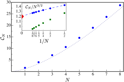
Figure 5: Contact of the ground state in the few- and many-body limit. Contact coefficient of the ground state at small positive $1/g$ as a function of $N$. The dots are the analytical results for $N\leq 3$ and numerical results for $4\leq N\leq 8$. We do not show a comparison between the ground-state contact and the perturbation evaluated within our approximate states, $\langle\left.{\tilde{\psi}_{N}}\right|{\cal H}^{\prime}\left|{\tilde{\psi}_{N}}\right>$, since the relative error between these is less than $0.05\%$ for $N\leq 8$. The dashed line is McGuire’s free-space solution mapped to the harmonic potential using the local density approximation — see the discussion in the main text. Inset: The ground-state contact coefficient in units of $N^{3/2}$ and plotted as a function of $1/N$ to illustrate the possible convergence to McGuire’s prediction (marked by a triangle). The dashed line is a cubic fit to our data. We also compare with the expectation value of Girardeau’s proposed ground state $\langle\left.{\psi_{\rm G}}\right|{\cal H}^{\prime}\left|{\psi_{\rm G}}\right>$ (green squares).

Approaching the many-body limit.

The fact that the wavefunction overlaps appear to extrapolate to a numerical value very close to 1 (see Fig. 2), indicates that our ansatz is highly accurate also in the many-body limit. Thus, we now investigate the limit $N\rightarrow\infty$ for the impurity ground state (48) at large repulsion. We focus on properties that depend on the impurity probability distribution in the bulk of the system.

The first such quantity is the contact coefficient, as shown in Fig. 5. We compare it with the expression ${\cal C}_{N}\approx 8\sqrt{2N^{3}}/(3\pi)$ corresponding to McGuire’s exact solution to the single impurity problem in free space McGuire (1965) mapped onto the harmonically confined system using the local density approximation Astrakharchik and Brouzos (2013). We see that our prediction for the contact appears to extrapolate to the Bethe ansatz result in the many-body limit, thus implying that the local density mapping is valid for the single-impurity ground-state energy. Indeed, this is consistent with the fact that the impurity ground-state wavefunction is confined to the central region of the trap (see Fig. 4) where the density of majority particles is highest.

We next calculate the probability density of the impurity in real space, $P_{N}(x_{0})=\int dx_{1}\cdots dx_{N}|\psi_{N}({\bf x})|^{2}$. This is very complicated to evaluate for general $N$, but in the thermodynamic limit $N\rightarrow\infty$, the probability distribution of the approximate ground-state wavefunction (48) may be converted into $P_{N}(x_{0})$. The distribution of majority particles is unaffected by the presence of the impurity in the thermodynamic limit, and according to the local density approximation it is $n(x)=\frac{1}{\pi}\sqrt{2\mu_{0}-x^{2}}$, where $\mu_{0}$ is the chemical potential at the center of the harmonic potential. This in turn yields $N=\int^{\sqrt{2\mu_{0}}}_{-\sqrt{2\mu_{0}}}n(x)dx=\mu_{0}$. The lattice index $i$ in the Heisenberg model corresponds to the number of majority particles to the left of the impurity; thus it may be related to the position in real space via $i=\int_{-\infty}^{x_{0}}n(x)$. Since $\int_{-\infty}^{0}n(x)=N/2$, we can then write:

$$\frac{i-N/2}{N} =\frac{1}{N}\int_{0}^{x_{0}}n(x)dx\simeq\frac{2x_{0}}{\pi\sqrt{2\mu_{0}}}$$ (49)

where we have taken the central part of the harmonic potential with $x_{0}\ll\sqrt{2\mu_{0}}$, Substituting this into Stirling’s approximation to the ground-state probability distribution, $P_{N}(i)\approx 2(\pi N)^{-1/2}\exp[-(2i-N)^{2}/N]$, finally yields the probability density of the impurity particle in the thermodynamic limit:

$$P_{N}(x_{0})\simeq\left(\frac{2}{\pi}\right)^{3/2}e^{-8x_{0}^{2}/\pi^{2}}.$$ (50)

Remarkably, upon tuning the system from the non-interacting ground state at $g=0^{+}$ with probability density $P_{\rm\tiny NI}(x_{0})=\exp(-x_{0}^{2})/\sqrt{\pi}$, the impurity wavefunction has only spread out slightly in the TG limit. The broader distribution may be viewed as an increase in the harmonic oscillator length by a factor $\pi/2\sqrt{2}$ or as a decreased effective mass. Note that our predicted probability density is completely different from that of the Girardeau state, $n(x_{0})/N$, which equals that of the ferromagnetic state. In particular, our predicted distribution retains a width $\sqrt{\left<x^{2}\right>}\sim 1$ for any $N$, while for the ferromagnetic state the width is $\sqrt{\left<x^{2}\right>}\sim\sqrt{N}$. The narrow width of the ansatz ground state compared with the length of the spin chain in turn implies that its overlap with the exact ground state wavefunction could approach 1 in the limit of large $N$. For instance, the overlap with a Gaussian of the same width indeed converges to 1 in the thermodynamic limit.

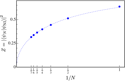
Figure 6: Emergence of the orthogonality catastrophe. Residue of the wavefunction $\psi_{N}$ as a function of $N$. For $N=1$ and $N=2$ we find the analytic results $2/\pi$ and $81/(16\pi^{2})$, respectively. The dashed line is $0.89/\sqrt{N+1}$. We do not show a comparison between the residue of the ground state in our approximation scheme and that of the exact ground state, as the relative error is less than $0.07\%$ for $N\leq 7$.

The small change in the ground-state impurity probability distribution from the non-interacting to the TG limit appears to suggest that the wavefunction of the system is only weakly perturbed by infinite interactions. On the other hand, it is well known that the system encounters the orthogonality catastrophe in the thermodynamic limit, where the state of the system has no overlap with the non-interacting state Anderson (1967). To reconcile these points, it is necessary to consider the impact of the interactions on the majority fermions, which reshuffle the Fermi sea. This is embedded in the residue $Z=|\langle\left.{\psi_{N}}\right|\psi_{\rm\tiny NI}\rangle|^{2}$, i.e. the squared overlap of the ground-state wavefunction with the non-interacting ground state at $g=0$:

$$\psi_{\rm\tiny NI}({\bf x}) =\frac{{\cal N}_{N-1}}{\pi^{1/4}}\left(\prod_{1\leq i<j\leq N}x_{ij}\right)e^{-\sum_{k=0}^{N}x_{k}^{2}/2}\ .$$ (51)

We compute the residue using a numerical method similar to that outlined in the Methods, and the result is shown in Fig. 6. By fitting, we find that the residue decreases with $N$ as $\sim 1/\sqrt{N+1}$. Intriguingly, the same scaling of the residue with particle number was predicted for a massive impurity immersed in a 1D Fermi gas in uniform space Castella (1996).

Higher energy manifolds and breathing modes.

We have demonstrated that our ansatz is extremely accurate for the $(N+1)$-dimensional ground-state manifold of the impurity problem to order $1/g$. We now show how it can be extended to states in higher energy manifolds. It is known that the 2D version of the Hamiltonian (1) is part of a “spectrum generating” $SO(2,1)$ algebra connected with scale transformations ${\mathbf{x}}\rightarrow{\mathbf{x}}/\lambda$ Pitaevskii and Rosch (1997). In 1D, this symmetry is broken for a finite interaction strength since the scaling of the interaction, $g\delta(x)\rightarrow\lambda g\delta(x)$, is different than in 2D. The key point, however, is that the $SO(2,1)$ symmetry is recovered in the TG limit $g\rightarrow\infty$. We can then use the technology developed for the $SO(2,1)$ symmetry, suitably adapted to the 1D case. In particular, one can define an operator $\hat{B}$ so that if $|n\rangle$ is an eigenstate with energy $E_{n}$, then $|n+1\rangle=\hat{B}^{\dagger}|n\rangle$ is an eigenstate with energy $E_{n+1}=E_{n}+2$ (see Methods). The spectrum in the TG limit therefore consists of towers of states separated by twice the harmonic potential frequency, where $\hat{B}|0\rangle=0$ for the lowest state in each tower.

Away from the TG limit, each level in these towers is shifted in energy, and Eq. (29) gives the energy shift of the ground-state manifold to a very good approximation. Each state in the ground-state manifold represents the lowest state in a separate tower of modes, and we now use the $SO(2,1)$ algebra to calculate the energy shift of the excited states in each tower. Within first order perturbation theory, the energy shift $\delta E_{n}$ of the $n$’th excited mode $|n\rangle$ away from its value in the TG limit is given by

$$\delta E_{n}=-\frac{1}{g}\frac{\langle 0|{\hat{B}}^{n}{\cal H}^{\prime}(\hat{B}^{\dagger})^{n}|0\rangle}{\langle 0|\hat{B}^{n}(\hat{B}^{\dagger})^{n}|0\rangle}.$$ (52)

Note that this result is exact to order $1/g$. The expectation values in Eq. (52) can be calculated using operator algebra only, once the so-called “scaling dimension” $\Delta_{{\cal H}^{\prime}}$ of ${\cal H}^{\prime}$ is known. Using Eq. (5), we find

$$\langle\bar{\phi}_{l}|{\cal H}^{\prime}|\bar{\phi}_{n}\rangle=\frac{1}{\lambda^{3}}\langle\phi_{l}|{\cal H}^{\prime}|\phi_{n}\rangle,$$ (53)

where $\bar{\phi}_{n}({\mathbf{x}})=\phi({\mathbf{x}}/\lambda)/\lambda^{(N+1)/2}$. It follows that the scaling dimension of ${\cal H}^{\prime}$ is $\Delta_{{\cal H}^{\prime}}=3$ in 1D. One can now use Eq. (52) to express the energy shift of the state $|n\rangle$ as a function of the energy shift of all lower states in the tower (see Methods). The simplest case is the energy shift $\delta E_{1}$ of the first excited breathing state $|1\rangle=\hat{B}^{\dagger}|0\rangle$, given by

$$\delta E_{1}=\left(1+\frac{3}{4E_{0}}\right)\delta E_{0},$$ (54)

where $\delta E_{0}$ is the energy shift of the $N+1$ particle ground state away from the value $E_{0}=N(N+2)/2$ in the TG limit. Equation (54) predicts that the energy shift of the first excited mode is larger than the shift of the state in the ground-state manifold. Physically, this means that the excited state energy approaches its non-interacting value faster than the ground state as one moves away from the TG limit. Used in combination with Eq. (29), Eq. (54) generalises our ansatz for the spectrum in the single impurity problem to higher energy manifolds. However, we emphasize that our results for the excited manifolds only depend on the energy levels in the ground state manifold, and are not limited to the impurity problem.

We can compare the prediction of Eq. (54) with the exact solution to the two-body problem. In 1D, the exact two-body energies $E$ are determined by the equation $\Gamma(3/4-E/2)/\Gamma(1/4-E/2)=-g/2\sqrt{2}$ Busch et al. (1998). Close to the TG limit $g\rightarrow\infty$, we have $E=3/2+\delta E_{0}$ for a state in the ground-state manifold and $E=7/2+\delta E_{1}$ for the first excited state in the tower, with $\delta E_{i}/E\ll 1$. Expanding the $\Gamma$ functions yields $\delta E_{1}/\delta E_{0}=3/2$, which is identical to the result obtained from Eq. (54) when using $E_{0}=3/2$. This demonstrates explicitly that Eq. (54), valid for any $N$, recovers the exact two-body theory close to the TG limit.

For large $N$, it immediately follows from Eq. (54) that the correction to the energy shift of the first excited manifold goes as $1/N^{2}$. Moreover, this holds for any $n\ll N$ (see Methods). Thus, in the thermodynamic limit we find that the dynamic $SO(2,1)$ symmetry extends to finite interactions, up to order $1/g$.

The lowest breathing mode frequency has been measured in several atomic gas experiments Kinast et al. (2004); Bartenstein et al. (2004); Vogt et al. (2012). The results in this section can therefore be tested experimentally providing a sensitive probe of interactions in the few-body system.

We note that the approach described in this section is exact to lowest order in $1/g$, and it is completely general. It would for instance be interesting to apply it to a system of 1D bosons close to the TG limit, where the frequency of the lowest breathing mode was recently calculated using a mapping to an effective fermionic Hamiltonian Zhang et al. (2014).

Radio-frequency spectroscopy.

Our results may be probed directly in cold atomic gases using radio-frequency (RF) spectroscopy, as already applied in the recent experiment Wenz et al. (2013). Consider a homogeneous RF-probe with frequency $\omega_{\rm rf}$ which flips the impurity atom from the hyperfine state $|a\rangle$ to the state $|b\rangle$. Within linear response, the RF signal is proportional to

$$\sum_{i,f}(P_{i}-P_{f})\left|\langle f|{\textstyle\int}dx\,\hat{\psi}_{b}^{\dagger}(x)\hat{\psi}_{a}(x)|i\rangle\right|^{2}\delta(\omega_{\rm rf}+E_{i}-E_{f}),$$

where $P_{i}(P_{f})$ is the probability of occupation of the initial $|i\rangle$ (final $|f\rangle$) many-body state, and $\hat{\psi}_{\sigma}$ is the field operator for the hyperfine state $|\sigma\rangle$.

Assume that the system initially is in a definite state $|i\rangle$ and that all final states are empty. There are two kinds of RF spectroscopy. In direct RF-spectroscopy, $a=\downarrow$ and the impurity atom interacts with the $\uparrow$ atoms in the initial state, which belongs to the interacting many-body ground-state manifold, whereas the final hyperfine state $|b\rangle$ of the impurity atom does not interact with the majority atoms. There will then be a peak at $\omega_{\rm rf}=-E_{0}$ in the RF spectrum in the TG limit, and the reduction of the height of the peak from its non-interacting value gives the quasiparticle residue of the initial state. There will also be peaks at $\omega_{\rm rf}=-E_{0}+2n$ with $n=1,2,\ldots$ as the initial interacting wavefunction has components in excited non-interacting states with the same parity. The shift of the peak position away from $\omega_{\rm rf}=-E_{0}$ gives the energy shift of the many-body ground state when $1/g>0$. In inverse RF spectroscopy, the initial state $|a\rangle$ of the impurity atom does not interact with the majority atoms whereas the final state does with $b=\downarrow$ Kohstall et al. (2011). There will then be a peak at $\omega_{\rm rf}=E_{0}$ in the RF spectrum in the TG limit and the shift in position when $1/g>0$ again gives the many-body energy shift directly. The reduction of the height of the peak from its non-interacting value gives the quasiparticle residue. There will also be RF peaks at higher frequencies corresponding to flipping into the excited interacting states.

Discussion

In this work, we investigated in detail the properties of a single impurity immersed in a Fermi sea of $N$ majority particles near the TG limit. By comparing with exact numerical results, we have demonstrated the impressive accuracy of our strong-coupling ansatz for arbitrary $N$. We have furthermore identified the effective Heisenberg Hamiltonian within which our ansatz is exact, and this has allowed us to evaluate analytically the entire ground-state manifold, yielding the discrete Chebyshev polynomials. In particular, the ground-state wavefunction from our ansatz at strong repulsion is a sign-alternating Pascal’s triangle in the spin chain. Since its overlap with the exact ground-state wavefunction extrapolates to a value $\sim 0.9999$ for $N\to\infty$, we believe that Eq. (48) is essentially indistinguishable from the result of numerically exact approaches.

In addition to the static properties considered here, our ansatz provides a framework for investigating impurity dynamics in a harmonic potential, since we have determined the entire spectrum of the ground-state manifold and associated excited states related via a scale transformation. The impurity dynamics in 1D gases have recently been investigated theoretically in Refs. Mathy et al. (2012); Kantian et al. (2014), and experimentally in Refs. Catani et al. (2012); Fukuhara et al. (2013).

Our results also extend far beyond the single-impurity problem since the effective Heisenberg Hamiltonian (30) accurately describes any number of $\uparrow,\,\downarrow$ particles in the strongly coupled regime, as explicitly demonstrated for $N_{\uparrow}=N_{\downarrow}=2$. For larger $N_{\uparrow}$ and $N_{\downarrow}$, where the number of states grows dramatically, our Hamiltonian can be tackled with numerical tools developed for lattice systems, such as the density matrix renormalization group White (1992), or matrix product states Affleck et al. (1988). Extending our approach beyond the two-component Fermi gas to other quantum mixtures would also enable us to address open problems in the context of quantum magnetism, such as the nature of correlations and dynamical quantum phase transitions. In particular, it would be interesting to investigate whether our ansatz may be extended to harmonically confined $N$-component fermions, a scenario which has relevance to $SU(N)$ magnetism Gorshkov et al. (2010) and which has recently been experimentally realized Pagano et al. (2014).

Finally, the exceptional accuracy of our simple ansatz and the suggestive form of the impurity spectrum $E-E_{0}\propto l(l+1)/g$, lead us to speculate that our results are the manifestation of a hidden approximate symmetry. This raises the tantalizing possibility that the 1D Fermi gas in a harmonic potential becomes near integrable in the strongly interacting limit.

Methods

Manipulations of the basis functions.

In order to calculate the overlaps of the basis functions $\phi_{l}$ it is useful to introduce an alternative formulation of the problem. First we note that, for a given ordering of particles, all basis functions $\phi_{l}$ (and consequently any superposition of these) are proportional to $\psi_{0}$. We may then define the complete and orthonormal set of basis states:

$$\langle{\bf x}\left|{\downarrow_{i}}\right>=\sqrt{N+1}\ \psi_{0}({\bf x})\Theta\left(\{x_{j}\}_{i}<x_{0}<\{x_{j}\}_{N-i}\right),$$ (55)

where $1\leq j\leq N$. $\{x_{j}\}_{i}$ corresponds to any set of $i$ spin-$\uparrow$ particles and the step function $\Theta$ is 1 if precisely $i$ of the $N$ majority particles are to the left of the impurity, and zero otherwise. Clearly the states described by Eq. (55) do not overlap. To see that they are properly normalized, consider

$$\langle\downarrow_{i}\left|{\downarrow_{i}}\right> =(N+1)\!\int\!d{\bf x}\ |\psi_{0}({\bf x})|^{2}\Theta\left(\{x_{j}\}_{i}<\!x_{0}\!<\{x_{j}\}_{N-i}\right)$$

$$=(N+1)\frac{N!}{(N+1)!}=1.$$ (56)

Here we used the fact that the integral over the (normalized) ferromagnetic state $\psi_{0}$ does not depend on the ordering of particles. Thus, restricting the integral to a particular ordering, the result is $1/(N+1)!$. Now, if $i$ particles are to the left of the impurity, there are ${{N}\choose{i}}$ ways of choosing these, with $i!\times(N-i)!$ ways of ordering those to the left and right of the impurity. Gathering the terms, the basis states $\{\left|\downarrow_{i}\right>\}$ are thus seen to form an orthonormal basis.

Recall now the definition of the basis states $\phi_{l}$:

$$\phi_{l} =\psi_{0}({\bf x})\sum_{1\leq i_{1}<\cdots<i_{l}\leq N}s_{i_{1}}\cdots s_{i_{l}},\hskip 14.22636pt1\leq l\leq N,$$ (57)

with $s_{j}\equiv\mbox{sign}(x_{j}-x_{0})$. Assuming there are exactly $i$ majority particles to the left of the impurity, we may evaluate the sum of sign functions:

$$\sum_{1\leq i_{1}<\cdots<i_{l}\leq N}s_{i_{1}}\cdots s_{i_{l}}=\sum_{k=0}^{l}(-1)^{k}\left(\begin{array}[]{c}i\\ k\end{array}\right)\left(\begin{array}[]{c}N-i\\ l-k\end{array}\right).$$ (62)

This simply counts how many combinations exist with $k$ [$l-k$] majority particles involved in the sign functions out of the $i$ [$N-i$] majority particles located to the left [right] of the impurity, respectively. Thus we arrive at the projection of the two sets of basis states:

$$\langle\left.{\downarrow_{i}}\right|\phi_{l}\rangle=\frac{1}{\sqrt{N+1}}\sum_{k=0}^{l}(-1)^{k}\left(\begin{array}[]{c}i\\ k\end{array}\right)\left(\begin{array}[]{c}N-i\\ l-k\end{array}\right).$$ (67)

The prefactor arises from the same arguments that led to Eq. (55).

The inner products $\Phi_{ln}=\langle\left.{\phi_{l}}\right|\phi_{n}\rangle$ then simply follow from Eq. (67),

$$\Phi_{ln}=\sum_{i=0}^{N}\langle\left.{\phi_{l}}\right|\downarrow_{i} \rangle\langle\downarrow_{i}\left|{\phi_{n}}\right>$$

$$=\frac{1}{N+1}\sum_{i=0}^{N} \left[\sum_{k_{1}=0}^{l}(-1)^{k_{1}}\left(\begin{array}[]{c}i\\ k_{1}\end{array}\right)\left(\begin{array}[]{c}N-i\\ l-k_{1}\end{array}\right)\right]$$ (72)

$$\times \left[\sum_{k_{2}=0}^{n}(-1)^{k_{2}}\left(\begin{array}[]{c}i\\ k_{2}\end{array}\right)\left(\begin{array}[]{c}N-i\\ n-k_{2}\end{array}\right)\right].$$ (77)

We also note that the matrix $\Phi$ is bisymmetric, i.e. $\Phi_{ln}=\Phi_{nl}=\Phi_{N-l,N-n}$.

Numerical evaluation of ${\cal H}^{\prime}$.

The matrix elements of ${\cal H}^{\prime}$ can be evaluated as

$${\cal H}^{\prime}_{ln} =\langle\left.{\phi_{l}}\right|{\cal H}^{\prime}\left|{\phi_{n}}\right>=\lim_{g\to\infty}g^{2}\sum_{i=1}^{N}\int d{\bf x}\ \delta(x_{i0})\phi_{l}\phi_{n}$$

$$=\sum_{i=1}^{N}\int d{\bf x}\ \delta(x_{i0})\left.\frac{\partial\phi_{l}}{\partial x_{i0}}\right|^{+}_{-}\left.\frac{\partial\phi_{n}}{\partial x_{i0}}\right|^{+}_{-},$$ (78)

where we have used the fact that $g\phi_{l}(x_{i0}=0)=\lim_{x_{i0}\to 0^{+}}\frac{\partial\phi_{l}}{\partial x_{i0}}(x_{i0})-\lim_{x_{i0}\to 0^{-}}\frac{\partial\phi_{l}}{\partial x_{i0}}(x_{i0})\equiv\frac{\partial\phi_{l}}{\partial x_{i0}}|_{-}^{+}$. This quantity can be non-zero due to the presence of cusps in the basis functions. Note that $\frac{\partial\phi_{0}}{\partial x_{i0}}|_{-}^{+}=0$ for the ferromagnetic state and therefore ${\cal H}^{\prime}_{0n}={\cal H}^{\prime}_{n0}=0$. This implies that $\phi_{0}$ is an eigenstate with $\mathcal{C}=0$, as expected.

We now show that the $(N+1)$-dimensional integrals appearing in the matrix elements of $\mathcal{H}^{\prime}$, Eq. (78), may conveniently be expressed in terms of a Taylor expansion of a suitable function. We begin by noting that the bracketed term of the wavefunction

$$\psi_{0}({\bf x}) ={\cal N}_{N}\left(\prod_{0\leq i<j\leq N}x_{ij}\right)e^{-\sum_{k=0}^{N}x_{k}^{2}/2},$$ (79)

only depends on the relative coordinates. It is then convenient to introduce the center-of-mass coordinate $x_{\rm cm}\equiv\sum_{i=0}^{N}x_{i}/(N+1)$, and relative coordinates $y_{0}=(N+1)(x_{0}-x_{\rm cm})$ and $y_{i}=x_{i0}$ $(1\leq i\leq N)$. The constraint $\sum_{i=0}^{N}x_{i}-(N+1)x_{\rm cm}=\sum_{i=0}^{N}y_{i}=0$ may be enforced through the use of a $\delta$-function, which in turn may be converted into an extra integral, yielding

$$\int d{\bf x}\ (\cdot)=\int\frac{dk}{2\pi}dx_{\rm cm}\,d\mathbf{y}\,e^{ik\sum_{j=0}^{N}y_{j}}\ (\cdot)$$

This allows us to decouple the center-of-mass coordinate. The integrand of Eq. (78) contains a factor of $e^{-\sum_{i=0}^{N}x_{i}^{2}}$ (following from the form of $\psi_{0}$), which may be written as $e^{-\sum_{i=1}^{N}y_{i}^{2}+y_{0}^{2}/(N+1)-(N+1)x_{\rm cm}^{2}}$. As this is the only term in which the center-of-mass coordinate appears in (78), $x_{\rm cm}$ may be integrated out to give $\sqrt{\frac{\pi}{N+1}}$.

Next consider the part of the integral involving both $k$ and $y_{0}$:

$$\int\frac{dk}{2\pi}dy_{0}\,(\cdot)e^{y_{0}^{2}/(N+1)}e^{iky_{0}}= \int\frac{dk}{2\pi}dy_{0}\,(\cdot)e^{-\nabla_{k}^{2}/(N+1)}e^{iky_{0}}$$

$$= \int dk\,\delta(k)\,e^{-\nabla_{k}^{2}/(N+1)}(\cdot),$$

where in the last step we have integrated by parts. Collecting all factors, we get an expression where the integrals over the $y_{i}$ have been decoupled:

$${\cal H}^{\prime}_{ln}= \sum_{i=1}^{N}\int d{\bf x}\ \delta(y_{i})\left.\frac{\partial\phi_{l}}{\partial y_{i}}\right|^{+}_{-}\left.\frac{\partial\phi_{n}}{\partial y_{i}}\right|^{+}_{-}$$

$$= 4N{\cal N}_{N}^{2}\sqrt{\frac{\pi}{N+1}}\int dk\,\delta(k)e^{-\nabla_{k}^{2}/(N+1)}$$

$$\times\left[\int d^{N-1}y\,e^{\sum_{j=1}^{N-1}(iky_{j}-y_{j}^{2})}S_{l-1}^{(N-1)}S_{n-1}^{(N-1)}\right.$$

$$\left.\hskip 28.45274pt\times\prod_{1\leq i_{1}<i_{2}<N}(y_{i_{1}}-y_{i_{2}})^{2}\prod_{1\leq m<N}y_{m}^{2}\right],$$ (80)

where $S_{l}^{(N)}\equiv\sum_{1\leq i_{1}<\cdots<i_{l}\leq N}s_{i_{1}}\cdots s_{i_{l}}\prod_{i=1}^{N}y_{i}$. We have made use of the fact that the integral is independent of $i$ so that we can differentiate with respect to just $y_{N}$ and multiply by $N$. We also used the relation $\left.\frac{\partial S_{l}^{(N)}}{\partial y_{N}}\right|^{+}_{-}=2S_{l-1}^{(N-1)}$. Denoting the quantity in square parentheses by $h_{ln}(k)$, and introducing its Taylor expansion around $k=0$, $h_{ln}(k)=\sum_{m=0}^{\infty}h_{ln}^{(m)}k^{m}$, we see that the desired matrix element is converted into a quickly convergent series, ${\cal H}^{\prime}_{ln}=4N{\cal N}_{N}^{2}\sqrt{\frac{\pi}{N+1}}\sum_{m=0}^{\infty}\left(\frac{-1}{N+1}\right)^{m}\frac{(2m)!}{m!}h_{ln}^{(2m)}$.

For the example of $N=3$, the function appearing in square parentheses for the matrix element ${\cal H}^{\prime}_{11}$ is $h_{11}(k)=\int dy_{1}\,dy_{2}\,e^{ik(y_{1}+y_{2})-y_{1}^{2}-y_{2}^{2}}y_{1}^{4}y_{2}^{4}(y_{1}-y_{2})^{2}$, while for the matrix element ${\cal H}^{\prime}_{31}$, it is $h_{31}(k)=\int dy_{1}\,dy_{2}\,e^{ik(y_{1}+y_{2})-y_{1}^{2}-y_{2}^{2}}|y_{1}y_{2}|y_{1}^{3}y_{2}^{3}(y_{1}-y_{2})^{2}$. In both cases we see how the integrals over the relative coordinates between the impurity and the majority particles separate. It is also easy to see that $h_{11}(k)=h_{33}(k)$, as expected.

Analytic solution for $\bm{N=3}$.

We start by considering the explicit solution of the Schrödinger equation perturbatively for $1/|g|\ll 1$. First, we note that the matrix elements of ${\cal H}^{\prime}$ can be written as

$${\cal H}^{\prime}_{ln} =4N\sum_{i=0}^{N-1}{\cal I}_{i}\left[\sum_{k_{1}=0}^{l-1}(-1)^{k_{1}}\left(\begin{array}[]{c}i\\ k_{1}\end{array}\right)\left(\begin{array}[]{c}N-1-i\\ l-1-k_{1}\end{array}\right)\right]$$ (85)

$$\times{{N-1}\choose{i}}\left[\sum_{k_{2}=0}^{n-1}(-1)^{k_{2}}\left(\begin{array}[]{c}i\\ k_{2}\end{array}\right)\left(\begin{array}[]{c}N-1-i\\ n-1-k_{2}\end{array}\right)\right].$$ (90)

where we have the integral

$${\cal I}_{i} =\int^{\infty}_{-\infty}dx_{0}\int^{x_{0}}_{-\infty}d^{i}x_{j}\int^{\infty}_{x_{0}}d^{N-1-i}x_{k}\left.\left(\frac{\partial\psi_{0}}{\partial x_{N0}}\right)^{2}\right|_{x_{N0}=0}$$

i.e., we integrate over $i$ of the majority particles to the left of the impurity, and $N-i-1$ to the right. Note that the integral only couples basis states with the same parity. One can also show that

$$\langle\left.{\phi_{N-l+1}}\right|{\cal H}^{\prime}\left|{\phi_{N-n+1}}\right>=\langle\left.{\phi_{l}}\right|{\cal H}^{\prime}\left|{\phi_{n}}\right>.$$

For $N=3$, it is possible to evaluate ${\cal I}_{i}$ analytically, thus giving

$${\cal H}^{\prime}_{11} ={\cal H}^{\prime}_{33}=\frac{475}{32\sqrt{2\pi}},$$

$${\cal H}^{\prime}_{13} ={\cal H}^{\prime}_{31}=\frac{1425\sqrt{2}\pi-56-2850\sqrt{2}\tan^{-1}\left(2\sqrt{2}\right)}{192\pi^{3/2}},$$

$${\cal H}^{\prime}_{22} =\frac{1425\sqrt{2}\pi-28-1425\sqrt{2}\tan^{-1}\left(2\sqrt{2}\right)}{48\pi^{3/2}}.$$ (91)

Combining this with the matrix of inner products $\Phi$ then allows us to solve the eigenvalue equation and determine $\mathcal{C}$ and $\psi$ analytically. The resulting expressions are rather cumbersome and yield the numerical values shown in the main text.

$SO(2,1)$ symmetry and excited states.

We define the scaling operator $\hat{S}(\lambda)$ as

$$\hat{S}(\lambda)\psi({\mathbf{x}})=\frac{\psi({\mathbf{x}}/\lambda)}{\lambda^{(N+1)/2}}.$$ (92)

It can be written as Nishida and Son (2007); Werner and Castin (2006)

$$\hat{S}(\lambda)=e^{-i\ln\lambda\hat{D}}\hskip 14.22636pt\text{ with }\hskip 14.22636pt\hat{D}=\frac{1}{2i}\sum_{j}(x_{j}\partial_{j}+\partial_{j}x_{j}).$$ (93)

The raising and lowering operators can then be defined as Moroz (2012)

$$\hat{B}=\hat{L}-\frac{\hat{Q}^{2}}{N+1}\hskip 14.22636pt\text{ with }\hskip 14.22636pt\hat{L}=\frac{1}{2}({\cal H}-\hat{X}^{2}-i\hat{D}),$$

for the $N+1$ particle state. Here $\hat{X}^{2}=\sum_{i}x_{i}^{2}$ is twice the harmonic potential, and $\hat{Q}=(\hat{P}+i\hat{K})/\sqrt{2}$ with $\hat{P}=\sum_{j}\hat{p}_{j}$ the total momentum and $\hat{K}=\sum_{j}x_{j}$ the center-of-mass coordinate. One can show that, in the TG limit, $[{\cal H},\hat{B}^{\dagger}]=2\hat{B}^{\dagger}$ from which it follows that if $|n\rangle$ is an eigenstate with energy $E_{n}$, then $|n+1\rangle=\hat{B}^{\dagger}|n\rangle$ is an eigenstate with energy $E_{n+1}=E_{n}+2$. The operator $\hat{B}^{\dagger}$ excites breathing modes, and the spectrum in the TG limit consists of towers of states separated by twice the harmonic potential frequency, where $\hat{B}|0\rangle=0$ for the lowest state in each tower.

To calculate the scaling dimension, we take the derivative of Eq. (53) with respect to $\lambda$ setting $\lambda=1$, from which it follows that the scaling dimension is $\Delta_{{\cal H}^{\prime}}=3$. The calculation of the energy shift, Eq. (52), is now rather long and cumbersome but straightforward since all necessary commutators are known Moroz (2012). We obtain

$$\delta E_{n}-\delta E_{n-1}=\frac{3}{4R_{n-1}}\delta E_{n-1}+\frac{R_{n-2}}{R_{n-1}}(\delta E_{n-1}-\delta E_{n-2}),$$ (94)

where we have defined $R_{n}=\sum_{j=0}^{n}E_{j}=\sum_{j=0}^{n}(E_{0}+2j)=(n+1)(E_{0}+n)$. Here $E_{j}$ is the internal energy of the $j$’th state, i.e the energy minus the zero point energy of the center-of-mass. The last term in Eq. (94) is zero for $n=1$. Equation (94) gives the shift $\delta E_{n}$ of the energy of the state $|n\rangle$ away from its value in the TG limit in terms of the energy shifts of the lower modes.

Acknowledgments: We gratefully acknowledge enlightening discussions with Selim Jochim and Gerhard Zürn on spin-polarized 1D experiments, and feedback on this work from Gareth Conduit, Frank Deuretzbacher, Vudtiwat Ngampruetikorn, David Petrosyan, Luis Santos, Richard Schmidt, Vijay Shenoy, Artem Volosniev, Zhenhua Yu, and Nikolaj Zinner. We thank Giuseppe Fedele for useful correspondence on discrete polynomials. Funding: P.M. acknowledges support from ERC AdG OSYRIS, EU EQuaM and IP SIQS, Plan Nacional FOQUS and the Ramón y Cajal programme, while M.M.P. acknowledges support from the EPSRC under Grant No. EP/H00369X/2. GMB would like to acknowledge the support of the Hartmann Foundation via grant A21352 and the Villum Foundation via grant VKR023163. J.L., P.M., and M.M.P. also wish to thank the Institute for Nuclear Theory at the University of Washington where this work was initiated. Finally, we wish to thank the ESF POLATOM network for financial support.

References

- Guan et al. (2013) X.-W. Guan, M. T. Batchelor, and C. Lee, Fermi gases in one dimension: From Bethe ansatz to experiments, Rev. Mod. Phys. 85, 1633 (2013).
- Busch et al. (1998) T. Busch, B.-G. Englert, K. Rzażewski, and M. Wilkens, Two Cold Atoms in a Harmonic Trap, Foundations of Physics 28, 549 (1998).
- Gharashi and Blume (2013) S. E. Gharashi and D. Blume, Correlations of the Upper Branch of 1D Harmonically Trapped Two-Component Fermi Gases, Phys. Rev. Lett. 111, 045302 (2013).
- Volosniev et al. (2014) A. G. Volosniev, D. V. Fedorov, A. S. Jensen, M. Valiente, and N. T. Zinner, Strongly interacting confined quantum systems in one dimension, Nat. Commun. 5, 5300 (2014).
- Deuretzbacher et al. (2014) F. Deuretzbacher, D. Becker, J. Bjerlin, S. M. Reimann, and L. Santos, Quantum magnetism without lattices in strongly interacting one-dimensional spinor gases, Phys. Rev. A 90, 013611 (2014).
- Bugnion and Conduit (2013) P. O. Bugnion and G. J. Conduit, Ferromagnetic spin correlations in a few-fermion system, Phys. Rev. A 87, 060502 (2013).
- Sowiński et al. (2013) T. Sowiński, T. Grass, O. Dutta, and M. Lewenstein, Few interacting fermions in a one-dimensional harmonic trap, Phys. Rev. A 88, 033607 (2013).
- Astrakharchik and Brouzos (2013) G. E. Astrakharchik and I. Brouzos, Trapped one-dimensional ideal Fermi gas with a single impurity, Phys. Rev. A 88, 021602 (2013).
- Guan et al. (2009) L. Guan, S. Chen, Y. Wang, and Z.-Q. Ma, Exact Solution for Infinitely Strongly Interacting Fermi Gases in Tight Waveguides, Phys. Rev. Lett. 102, 160402 (2009).
- Girardeau (2010) M. D. Girardeau, Two super-Tonks-Girardeau states of a trapped one-dimensional spinor Fermi gas, Phys. Rev. A 82, 011607 (2010).
- Cui and Ho (2014) X. Cui and T.-L. Ho, Ground-state ferromagnetic transition in strongly repulsive one-dimensional Fermi gases, Phys. Rev. A 89, 023611 (2014).
- Paredes et al. (2004) B. Paredes, A. Widera, V. Murg, O. Mandel, S. Folling, I. Cirac, G. V. Shlyapnikov, T. W. Hansch, and I. Bloch, Tonks-Girardeau gas of ultracold atoms in an optical lattice, Nature 429, 277 (2004).
- Kinoshita et al. (2004) T. Kinoshita, T. Wenger, and D. S. Weiss, Observation of a One-Dimensional Tonks-Girardeau Gas, Science 305, 1125 (2004).
- Serwane et al. (2011) F. Serwane, G. Zürn, T. Lompe, T. B. Ottenstein, A. N. Wenz, and S. Jochim, Deterministic Preparation of a Tunable Few-Fermion System, Science 332, 336 (2011).
- Zürn et al. (2012) G. Zürn, F. Serwane, T. Lompe, A. N. Wenz, M. G. Ries, J. E. Bohn, and S. Jochim, Fermionization of Two Distinguishable Fermions, Phys. Rev. Lett. 108, 075303 (2012).
- Wenz et al. (2013) A. N. Wenz, G. Zürn, S. Murmann, I. Brouzos, T. Lompe, and S. Jochim, From Few to Many: Observing the Formation of a Fermi Sea One Atom at a Time, Science 342, 457 (2013).
- Zürn et al. (2013) G. Zürn, A. N. Wenz, S. Murmann, A. Bergschneider, T. Lompe, and S. Jochim, Pairing in Few-Fermion Systems with Attractive Interactions, Phys. Rev. Lett. 111, 175302 (2013).
- Murmann et al. (2015) S. Murmann, A. Bergschneider, V. M. Klinkhamer, G. Zürn, T. Lompe, and S. Jochim, Two Fermions in a Double Well: Exploring a Fundamental Building Block of the Hubbard Model, Phys. Rev. Lett. 114, 080402 (2015).
- Matveev (2004) K. A. Matveev, Conductance of a Quantum Wire in the Wigner-Crystal Regime, Phys. Rev. Lett. 92, 106801 (2004).
- Matveev and Furusaki (2008) K. A. Matveev and A. Furusaki, Spectral Functions of Strongly Interacting Isospin- Bosons in One Dimension, Phys. Rev. Lett. 101, 170403 (2008).
- Anderson (1967) P. W. Anderson, Infrared Catastrophe in Fermi Gases with Local Scattering Potentials, Phys. Rev. Lett. 18, 1049 (1967).
- Christandl et al. (2004) M. Christandl, N. Datta, A. Ekert, and A. J. Landahl, Perfect State Transfer in Quantum Spin Networks, Phys. Rev. Lett. 92, 187902 (2004).
- Eisert et al. (2015) J. Eisert, M. Friesdorf, and C. Gogolin, Quantum many-body systems out of equilibrium, Nature Physics 11, 124 (2015).
- Girardeau et al. (2001) M. D. Girardeau, E. M. Wright, and J. M. Triscari, Ground-state properties of a one-dimensional system of hard-core bosons in a harmonic trap, Phys. Rev. A 63, 033601 (2001).
- Deuretzbacher et al. (2008) F. Deuretzbacher, K. Fredenhagen, D. Becker, K. Bongs, K. Sengstock, and D. Pfannkuche, Exact Solution of Strongly Interacting Quasi-One-Dimensional Spinor Bose Gases, Phys. Rev. Lett. 100, 160405 (2008).
- Lieb and Mattis (1962) E. Lieb and D. Mattis, Theory of Ferromagnetism and the Ordering of Electronic Energy Levels, Phys. Rev. 125, 164 (1962).
- Olshanii and Dunjko (2003) M. Olshanii and V. Dunjko, Short-Distance Correlation Properties of the Lieb-Liniger System and Momentum Distributions of Trapped One-Dimensional Atomic Gases, Phys. Rev. Lett. 91, 090401 (2003).
- Tan (2008) S. Tan, Energetics of a strongly correlated Fermi gas, Annals of Physics 323, 2952 (2008).
- Barth and Zwerger (2011) M. Barth and W. Zwerger, Tan relations in one dimension, Annals of Physics 326, 2544 (2011).
- Volosniev et al. (2015) A. G. Volosniev, D. Petrosyan, M. Valiente, D. V. Fedorov, A. S. Jensen, and N. T. Zinner, Engineering the dynamics of effective spin-chain models for strongly interacting atomic gases, Phys. Rev. A 91, 023620 (2015).
- Beals and Wong (2010) R. Beals and R. Wong, Special functions: A Graduate Text (Cambridge University Press, Cambridge UK, 2010).
- McGuire (1965) J. B. McGuire, Interacting Fermions in One Dimension. I. Repulsive Potential, Journal of Mathematical Physics 6, 432 (1965).
- Castella (1996) H. Castella, Effect of finite impurity mass on the Anderson orthogonality catastrophe in one dimension, Phys. Rev. B 54, 17422 (1996).
- Pitaevskii and Rosch (1997) L. P. Pitaevskii and A. Rosch, Breathing modes and hidden symmetry of trapped atoms in two dimensions, Phys. Rev. A 55, R853 (1997).
- Kinast et al. (2004) J. Kinast, S. L. Hemmer, M. E. Gehm, A. Turlapov, and J. E. Thomas, Evidence for Superfluidity in a Resonantly Interacting Fermi Gas, Phys. Rev. Lett. 92, 150402 (2004).
- Bartenstein et al. (2004) M. Bartenstein, A. Altmeyer, S. Riedl, S. Jochim, C. Chin, J. H. Denschlag, and R. Grimm, Collective Excitations of a Degenerate Gas at the BEC-BCS Crossover, Phys. Rev. Lett. 92, 203201 (2004).
- Vogt et al. (2012) E. Vogt, M. Feld, B. Fröhlich, D. Pertot, M. Koschorreck, and M. Köhl, Scale Invariance and Viscosity of a Two-Dimensional Fermi Gas, Phys. Rev. Lett. 108, 070404 (2012).
- Zhang et al. (2014) Z. D. Zhang, G. E. Astrakharchik, D. C. Aveline, S. Choi, H. Perrin, T. H. Bergeman, and M. Olshanii, Breakdown of scale invariance in the vicinity of the Tonks-Girardeau limit, Phys. Rev. A 89, 063616 (2014).
- Kohstall et al. (2011) C. Kohstall, M. Zaccanti, M. Jag, A. Trenkwalder, P. Massignan, G. M. Bruun, F. Schreck, and R. Grimm, Metastability and coherence of repulsive polarons in a strongly interacting Fermi mixture, Nature 485, 615 (2011).
- Mathy et al. (2012) C. J. M. Mathy, M. B. Zvonarev, and E. Demler, Quantum flutter of supersonic particles in one-dimensional quantum liquids, Nature Physics 8, 881 (2012).
- Kantian et al. (2014) A. Kantian, U. Schollwöck, and T. Giamarchi, Competing Regimes of Motion of 1D Mobile Impurities, Phys. Rev. Lett. 113, 070601 (2014).
- Catani et al. (2012) J. Catani, G. Lamporesi, D. Naik, M. Gring, M. Inguscio, F. Minardi, A. Kantian, and T. Giamarchi, Quantum dynamics of impurities in a one-dimensional Bose gas, Phys. Rev. A 85, 023623 (2012).
- Fukuhara et al. (2013) T. Fukuhara, A. Kantian, M. Endres, M. Cheneau, P. Schauß, S. Hild, D. Bellem, U. Schollwöck, T. Giamarchi, C. Gross, I. Bloch, and S. Kuhr, Quantum dynamics of a mobile spin impurity, Nature Physics 9, 235 (2013).
- White (1992) S. R. White, Density matrix formulation for quantum renormalization groups, Phys. Rev. Lett. 69, 2863 (1992).
- Affleck et al. (1988) I. Affleck, T. Kennedy, E. Lieb, and H. Tasaki, Valence bond ground states in isotropic quantum antiferromagnets, Communications in Mathematical Physics 115, 477 (1988).
- Gorshkov et al. (2010) A. V. Gorshkov, M. Hermele, V. Gurarie, C. Xu, P. S. Julienne, J. Ye, P. Zoller, E. Demler, M. D. Lukin, and A. M. Rey, Two-orbital SU(N) magnetism with ultracold alkaline-earth atoms, Nature Physics 6, 289 (2010).
- Pagano et al. (2014) G. Pagano, M. Mancini, G. Cappellini, P. Lombardi, F. Schäfer, H. Hu, X.-J. Liu, J. Catani, C. Sias, M. Inguscio, and L. Fallani, A one-dimensional liquid of fermions with tunable spin, Nature Physics 10, 198 (2014).
- Nishida and Son (2007) Y. Nishida and D. T. Son, Nonrelativistic conformal field theories, Phys. Rev. D 76, 086004 (2007).
- Werner and Castin (2006) F. Werner and Y. Castin, Unitary gas in an isotropic harmonic trap: Symmetry properties and applications, Phys. Rev. A 74, 053604 (2006).
- Moroz (2012) S. Moroz, Scale-invariant Fermi gas in a time-dependent harmonic potential, Phys. Rev. A 86, 011601 (2012).