An Experimental Test of Envariance

Abstract

Envariance, or environment-assisted invariance, is a recently identified symmetry for maximally entangled states in quantum theory with important ramifications for quantum measurement, specifically for understanding Born’s rule zurek03.1 ; zurek03.2 ; zurek05 . We benchmark the degree to which nature respects this symmetry by using entangled photon pairs. Our results show quantum states can be $(99.66\pm 0.04)\%$ envariant as measured using the quantum fidelity jozsa94 , and $(99.963\pm 0.005)\%$ as measured using a modified Bhattacharya Coefficient bhattacharyya43 , as compared with a perfectly envariant system which would be 100% in either measure. The deviations can be understood by the less-than-maximal entanglement in our photon pairs.

Symmetries play a central role in physics with wide-reaching implications in fields as diverse as spectroscopy and particle physics. It is therefore of fundamental importance to identify and understand new symmetries of nature. One of these more recently identified symmetrys in quantum mechanics has been named environment-assisted invariance, or envariance zurek03.1 . It applies in certain cases where a composite quantum object consists of a system part, labelled $\mathsf{S}$, and an environment part, labelled $\mathsf{E}$. If some action is applied to the system part only, described by some unitary transformation, $U_{\mathsf{S}}$, then the state is said to be envariant under $U_{\mathsf{S}}$ if another unitary applied to the environment, $U_{\mathsf{E}}$, can restore the initial state. This can be expressed,

$$U_{\mathsf{S}}|\psi_{\mathsf{SE}}\rangle = (u_{\mathsf{S}}\otimes\mathbb{1}_{\mathsf{E}})|\psi_{\mathsf{SE}}\rangle=|\eta_{\mathsf{SE}}\rangle$$ (1)

$$U_{\mathsf{E}}|\eta_{\mathsf{SE}}\rangle = (\mathbb{1}_{\mathsf{S}}\otimes u_{\mathsf{E}})|\eta_{\mathsf{SE}}\rangle=|\psi_{\mathsf{SE}}\rangle.$$ (2)

Envariance is an example of an assisted symmetry zurek05 where once the system is transformed under some unitary $U_{\mathsf{S}}$, it can be restored to its original state by another operation on a physically distinct system: the environment.

Envariance is a uniquely quantum symmetry in the following sense. A pure quantum state represents complete knowledge of the quantum system. In an entangled quantum state, however, complete knowledge of the whole system does not imply complete knowledge of its parts. It is therefore possible that an operation on one part of a quantum state can alter the global state, but its local effects are masked by incomplete knowledge of that part; the effect on the global state can then be undone by an action on a different part. In contrast, complete knowledge of a composite classical system implies complete knowledge of each of its parts. Thus transforming one part of a classical system cannot be masked by incomplete knowledge and cannot be undone by a change on another part.

Envariance plays a prominent role in work related to fundamental issues of decoherence and quantum measurement zurek03.1 ; zurek03.2 ; zurek05 . Decoherence converts amplitudes in coherent superposition states to probabilities in mixtures and is central to the emergence of the classical world from quantum mechanics zurek91 ; schlosshauer05 . Mathematically the mixture appears in the reduced density operator of the system which is extracted from the global wavefunction by a partial trace landau27 ; nielsen00 . This partial trace limits the approach for deriving, as opposed to separately postulating, the connection between the wavefunction and measurement probabilities known as Born’s rule born26 , since the partial trace assumes Born’s rule is valid zurek03.1 ; schlosshauer03 . Envariance was employed in a derivation of Born’s rule which sought to avoid circularity inherent to approaches which rely on partial trace zurek03.1 . For comments on this derivation, see for example schlosshauer03 ; barnum03 ; mohrhoff04 .

In the present work, we subject envariance to experimental test in an optical system. We use the polarization of a single photon to encode the system, $\mathsf{S}$, and the polarization of a second single photon to encode the environment, $\mathsf{E}$. We subject the system photon to a wide range of polarization rotations with the goal of benchmarking the degree to which we can restore the initial state by applying a second transformation on the environment photon.

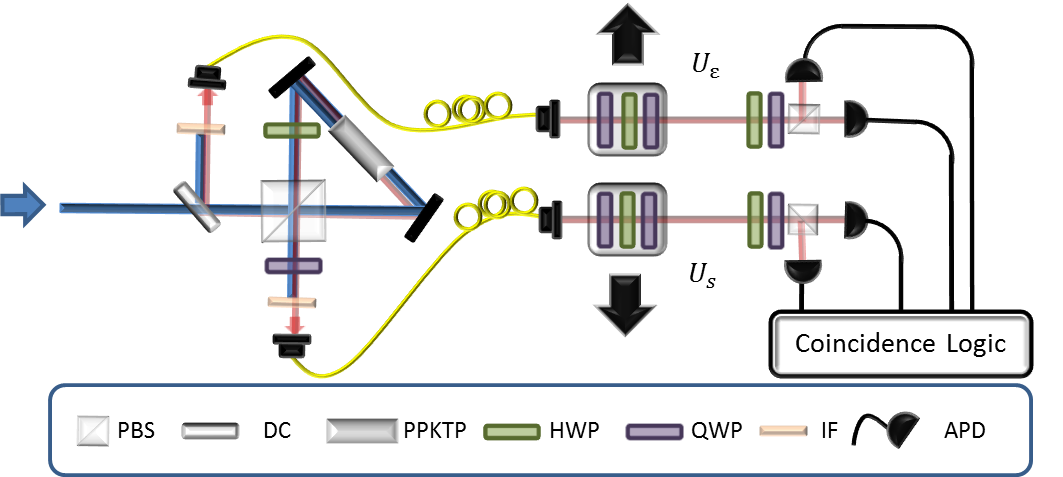
Figure 1: Experimental setup. The entangled photon pairs are created using type-II spontaneous parametric down-conversion. The pump laser is focused on a periodically-poled KTP crystal and pairs of entangled photons with anti-correlated polarizations are emitted. The pump is filtered using a band-pass filter, and polarization controls adjust for the alterations due to the coupling fibres. The entangled photon pairs are set so one photon is considered the system, and the other is considered the environment. After the source the unitary transformations are applied. A three wave plate combination is required to apply an arbitrary unitary transformation: quarter wave-plate (QWP), half wave-plate (HWP), QWP. A set of this combination of wave plates is mounted on each translation stage which can slide the wave plates in and out of the path of the incoming photons. The photons are then detected using polarizing beam splitters (PBS) and two wave plates to take projective measurements. The counts are then analyzed using coincidence logic.

Our test requires a source of high-quality two-photon polarization entanglement, an optical set-up to perform unitary operations on zero, one, or both of the photons, and polarization analyzers to characterize the final state of the light. Our experimental setup is shown in Fig. 1. We produce pairs of polarization-entangled photons using spontaneous parametric down-conversion (SPDC) in a Sagnac interferometer kim06 ; fedrizzi07 ; biggerstaff09 . In the ideal case, this source produces pairs of photons in the singlet state,

$$|\psi_{\mathsf{SE}}\rangle=\frac{1}{\sqrt{2}}\left(|H\rangle_{\mathsf{S}}|V\rangle_{\mathsf{E}}-|V\rangle_{\mathsf{S}}|H\rangle_{\mathsf{E}}\right),$$ (3)

where $|H\rangle$ ($|V\rangle$) represents horizontal (vertical) polarization, and $\mathsf{S}$ and $\mathsf{E}$ label the photons. This state is envariant under all unitary transformations and has the convenient symmetry that $u_{\mathsf{S}}=u_{\mathsf{E}}$ for all $u_{\mathsf{S}}$. We pump a $10$ mm periodically-poled KTP crystal (PPKTP), phase-matched to produce photon pairs at $809.8$ nm and $809.3$ nm from type-II down-conversion using $6$ mW from a CW diode pump laser with centre wavelength $404.8$ nm. The output from the source is coupled into single-mode fibres, where polarization controllers correct unwanted polarization rotations in the fibre. The light is coupled out of the fibres and directed to two independent polarization analyzers. Each analyzer consists of a half-wave plate (HWP), quarter-wave plate (QWP), and a polarizing beam-splitter (PBS). Between the fibre and the analyzers are two sets of wave plates—a QWP, a HWP, then another QWP—which can be inserted as a group into the beam paths to implement controlled polarization transformations. Photons from both ports of each PBS are detected using single-photon counting modules (Perkin-Elmer SPCM-AQ4C) and analyzed using coincidence logic with a $1$ ns coincidence window, counting for $5$ s. We typically measured total coincidence rates of $5.4$ kHz across the four detection possibilities for photons $\mathsf{S}$ and $\mathsf{E}$.

Rotation Axis	$\alpha(\theta)$	$\beta(\theta)$	$\gamma(\theta)$
$\hat{x}$	$\pi/2$	$-\theta/4$	$\pi/2$
$\hat{y}$	$\pi/2+\theta/2$	$\theta/4$	$\pi/2$
$\hat{z}$	$\pi/4$	$-\pi/4-\theta/4$	$\pi/4$

Table 1: Wave plate settings used to implement polarization rotations. The angles $\alpha$, $\beta$ and $\gamma$ are the wave plate angles for the first QWP, the HWP and the second QWP respectively. The angle $\theta$ is the rotation angle of the polarization about the specified axis on the Bloch sphere.

For our experiment, we implemented rotations about the standard $\hat{x}$, $\hat{y}$, and $\hat{z}$ axes of the Bloch sphere; in addition we implemented rotations about an axis $\hat{m}=(\hat{x}+\hat{y}+\hat{z})/\sqrt{3}$. The wave plate angles used to implement rotations by an angle $\theta$ about the $\hat{x}$, $\hat{y}$, and $\hat{z}$ axes are shown in Table 1; the angles to implement rotations about $\hat{m}$ were determined numerically using Mathematica.

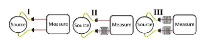
Figure 2: Experimental measurement procedure. We investigated the impact of each unitary transformation by performing quantum state tomography at three different stages: directly on the initial state with no unitary transformations (I), on the state with a transformation applied to the system photon (II), and on a state with the same transformation applied to both the system and environment photon (III).

Our experiment proceeds in three stages as depicted in Fig. 2: first characterizing the initial state (I), then characterizing the state after a transformation is applied to the system photon (II), and finally characterizing the state after that same transformation is applied to both system and environment (III). We record a tomographically-overcomplete set of measurements at each stage, performing the 36 combinations of the polarization measurements, $|H\rangle$, $|V\rangle$, $|D\rangle$=$(|H\rangle+|V\rangle)/\sqrt{2}$, $|A\rangle$=$(|H\rangle-|V\rangle)/\sqrt{2}$, $|R\rangle$=$(|H\rangle+i|V\rangle)/\sqrt{2}$, and $|L\rangle$=$(|H\rangle-i|V\rangle)/\sqrt{2}$ on each photon and counting for $5$ s for each setting. The states were then reconstructed using the maximum likelihood method from Ref. jezek03 . This procedure was repeated for a diverse range of transformations. We configured our setup to implement unitary rotations in multiples of 30^∘ from 0^∘ to 360^∘ about each of the $\hat{x}$, $\hat{y}$, $\hat{z}$, and $\hat{m}$ axes. The data acquisition time for this procedure over the set of 13 rotation angles about each axis was approximately six hours. The source was realigned before each run to achieve maximum fidelity with the singlet state from $0.985$ to $0.990$.

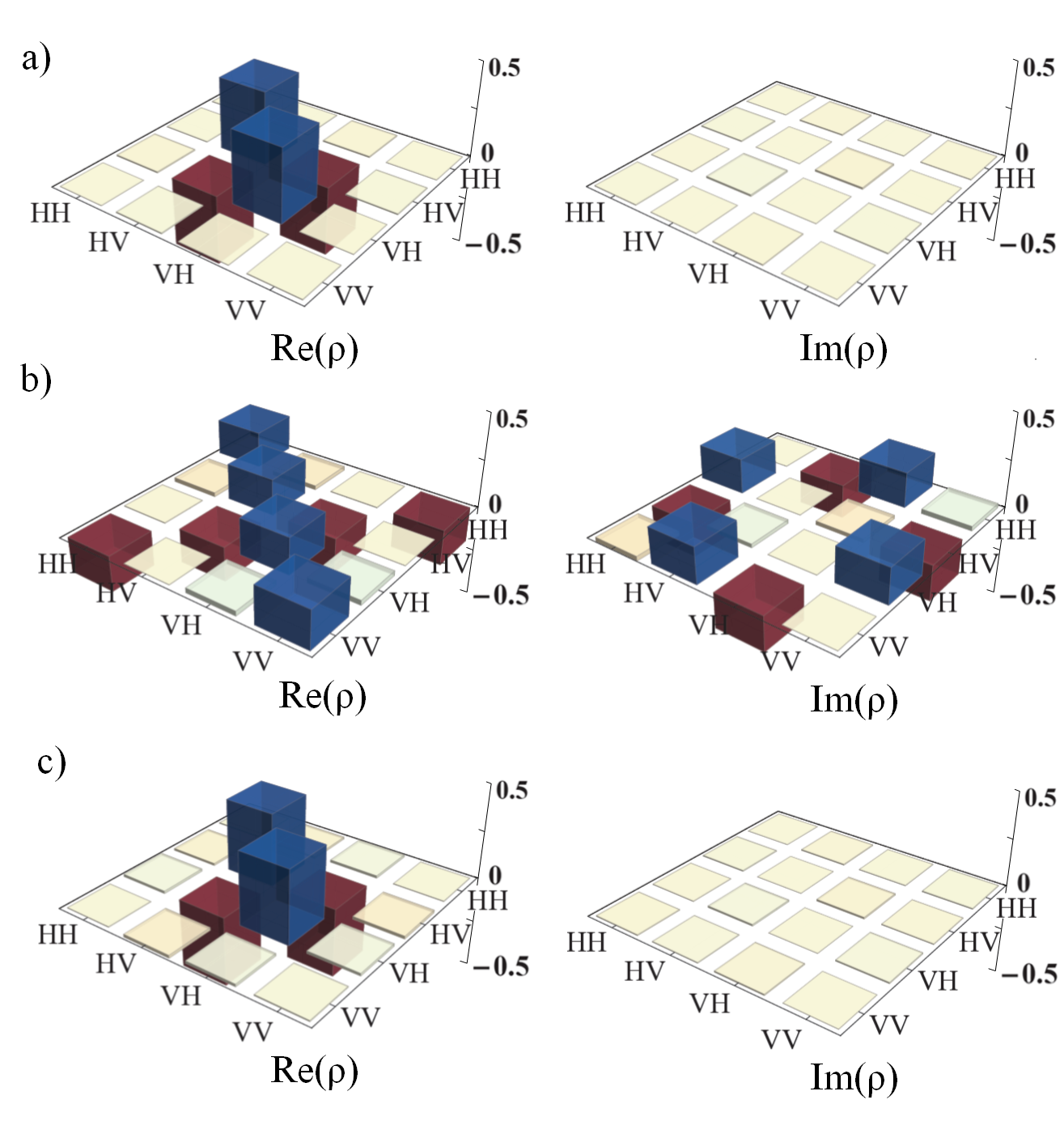
Figure 3: a) Is the real and imaginary parts of the reconstructed density matrix of the initial state from the source (stage I of the procedure). It has $0.987$ fidelity jozsa94 with the ideal. b) The system photon is transformed using wave plates set to implement the rotation of $90^{\circ}$ about the $\hat{x}$ axis, stage II. The resulting density matrix shown has $0.488$ fidelity with the ideal initial state,$0.501$ with the initial reconstructed state and $0.995$ with the expected state, calculated by transforming the density matrix from a). c) The reconstructed density matrix after the same unitary from b) is applied to both photons, stage III. This state has a $0.987$ fidelity with the ideal, $0.995$ with the reconstructed state from a), and $0.997$ with the expected state calculated by transforming the state from part a).

Figure  3a)–c) show the real and imaginary parts of the reconstructed density matrix of the quantum state at the three stages in the experiment, I, II, and III respectively. The fidelity jozsa94 of the state with the ideal $\psi^{-}\rangle$ state during these samples of two of the stages are $0.987$ for both I a), and III c), respectively, and is defined as jozsa94 :

$$F(\rho,\sigma)={\{\mathrm{Tr}[(\sqrt{\rho}\sigma\sqrt{\rho})^{1/2}]\}}^{2}$$ (4)

We can use this definition to calculate the fidelity between the state at stages I and III. Comparing between the states shown in Fig. 3 panels a) and c) the resulting fidelity is $0.995$.

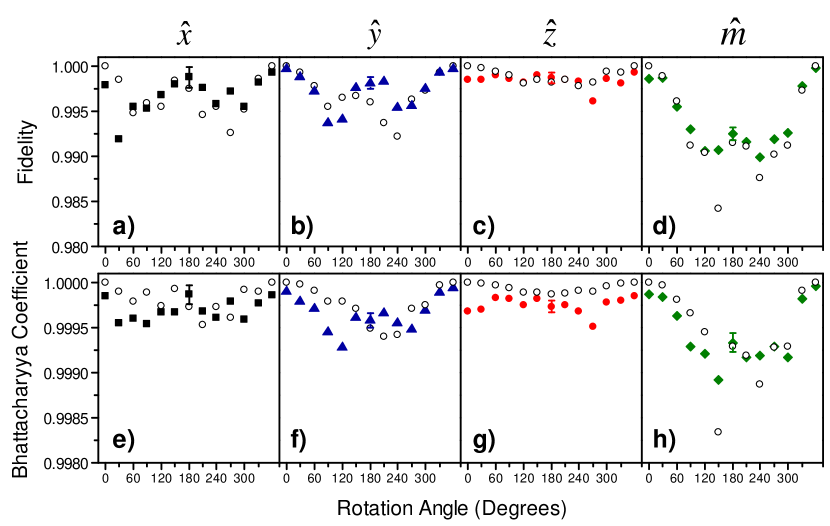
Figure 4: Analysis of the experimental results. Panels a)–d) show the fidelity analysis results for unitary rotations about $\hat{x}$, $\hat{y}$, $\hat{z}$, and $\hat{m}$ axes as functions of rotation angle. The coloured data points are the comparison between stage I and stage III (comparing the source state and the state after the unitary has been applied to both qubits). The open circles show a theoretical comparison. Panels e)–h) show the quantum Bhattacharyya results comparing stage I and stage III in the coloured data points for each of the four axis, with the open circles being the theoretical comparison. For plots which include a comparison of stage I and II (applying the unitary to one qubit only) and theoretical comparisons, see the appendix. The error bar for each graph is the standard deviation of comparisons of source state measurements during the experiment.

The summary of the results from our experiment is shown in Fig. 4. The coloured data points in Fig. 4a)–d) show the fidelity of the experimentally reconstructed state at stage III with the reconstructed state from the initial stage I, i.e., $F(\rho_{\rm{expt}}^{\mathbf{I}},\rho_{\rm{expt}}^{\mathbf{III}})$, as a function of the rotation angle for rotations about the $\hat{x}$, $\hat{y}$, $\hat{z}$, and $\hat{m}$, respectively. The open circles show the theoretical expectation for the fidelity between the measured state at stage I with the expected state in stage III, calculated by acting the unitaries on the measured state from stage I, i.e., $F(\rho_{\rm{expt}}^{\mathbf{I}},\rho_{\rm{th}}^{\mathbf{III}})$. The fidelities are very high, close to the limit of 1, in all cases and we see reasonable agreement with expectation.

We considered the effects of Poissonian noise and waveplate calibration on our results and found that these effects were too small to explain the deviation between $F(\rho_{\rm{expt}}^{\mathbf{I}},\rho_{\rm{expt}}^{\mathbf{III}})$ and $F(\rho_{\rm{expt}}^{\mathbf{I}},\rho_{\rm{th}}^{\mathbf{III}})$. To account for this, we characterized the fluctuations in the state produced by the source itself by comparing the state produced in subsequent stage I sates in the data collection; recall that stage I for each choice of unitary is always the same (no additional waveplates inserted) and thus provides a good measure of the source stability. Specifically, we calculated the standard deviation in the fidelity of the state produce at a stage I in the $i^{\rm{th}}$ round of the experiment to that produced in the next, $(i+1)^{\rm{th}}$, stage I, $F(\rho_{\rm{expt}}^{\mathbf{I},i},\rho_{\rm{expt}}^{\mathbf{I},i+1})$. The standard deviation in these fidelities calculated from the data taken within each set of rotation axes are shown as representative error bars on the plots in Figs. 4a)–d). The standard deviation of this quantity over all the experiments was $0.0008$. We characterize the difference between the measured and expected fidelities by calculating the standard deviation in the quantity, $F(\rho_{\rm{expt}}^{\mathbf{I}},\rho_{\rm{expt}}^{\mathbf{III}})-F(\rho_{\rm{expt}}^{\mathbf{I}},\rho_{\rm{th}}^{\mathbf{III}})$, for each experiment. (This is the difference between the coloured and open data points in Figs. 4a)–d).) over all experiments to be $0.002$. This value is comparable to the error in the fidelity due to source fluctuations. Refer to the appendix to see the comparison between stage I and stage II, which would not fit on the scale of Fig. 4.

From our data, we extract the average fidelity $F(\rho_{\rm{expt}}^{\mathbf{I}},\rho_{\rm{expt}}^{\mathbf{III}})$ for the set of measurements made for each unitary axis and show the results in Table II. As measured by the average fidelity, our experiment benchmarks envariance to $0.9966\pm 0.0004$,($(99.66\pm 0.04)\%$ of the ideal) averaged over all rotations.

Rotation Axis	Average Fidelity	Average $BC$
$\hat{x}$	$0.997\pm 0.001$	$0.9997\pm 0.0001$
$\hat{y}$	$0.9973\pm 0.0007$	$0.99966\pm 0.00008$
$\hat{z}$	$0.9984\pm 0.0006$	$0.99975\pm 0.00007$
$\hat{m}$	$0.9941\pm 0.0007$	$0.9994\pm 0.0001$
Overall average:	$0.9966\pm 0.0004$	$0.99963\pm 0.00005$

Table 2: Summary of the results for comparing stages I and III using fidelity and Bhattacharyya Coefficient ($BC$) analysis and averaging over each unitary rotation. The overall average is representative of the overall envariance of our state.

Fidelity has conceptual problems as a measure for testing quantum mechanics, since the density matrix we used to compute the fidelity is reconstructed using state tomography, which is under the assumption of Born’s rule. The Bhattacharyya Coefficient ($BC$) is a measure of the overlap between two discrete distributions $P$ and $Q$, where $p_{i}$ and $q_{i}$ are the probabilities of the $i^{th}$ element for $P$ and $Q$ respectively. The $BC$ is defined bhattacharyya43 ,

$$BC=\sum_{i}\sqrt{p_{i}q_{i}}.$$ (5)

If we normalize the measured tomographic data by dividing by the sum of the counts, we can treat this as a probability distribution. The $BC$ then can be calculated using the distribution of measurements at each stage in the experiment, directly analogous to the approach used with fidelity. It should be noted that the $BC$ has some limitations when applied in this case. If two quantum states produce identical measurement outcomes, its value is 1. Unlike fidelity though, it is not the case that the $BC$ goes to 0 for orthogonal quantum states. For example, the $BC$ for two orthogonal Bell states measured with an overcomplete set of polarization measurements is $7/9$. Furthermore, the value of the $BC$ is dependent on the particular choice of measurements taken. While we are employing a commonly-used measurement set for characterizing two qubits, other choices would produce different $BC$s. Nevertheless, this metric can be employed to quantify the envariance in our experiment without quantum assumptions, making it appropriate for testing quantum mechanics.

The Bhattacharyya Coefficients from our measured data are shown in Fig. 4e)–h). We normalize the measured counts from stages I and III to give us probability distributions $p^{\mathbf{I}}_{\rm{expt}}$ and $p^{\mathbf{III}}_{\rm{expt}}$. The coloured data points in Figs. 4e)–h) show the $BC$ between these distributions, $BC(p_{\rm{expt}}^{\mathbf{I}},p_{\rm{expt}}^{\mathbf{III}})$. The open circles are a theoretical expectation of the $BC$ given the tomographic measurements from stage I; for these theoretical values we used state tomography, and thus assumed quantum mechanics, to obtain the expected distribution $p_{\rm{th}}^{\mathbf{III}}$ and calculate the expected $BC$, $BC(p_{\rm{expt}}^{\mathbf{I}},p_{\rm{th}}^{\mathbf{III}})$.

Using an analogous procedure to that employed with the fidelity, we estimate the uncertainty in the $BC$ by comparing subsequent measured distributions in stage I throughout the experiment, i.e., $BC(p_{\rm{expt}}^{\mathbf{I},i},p_{\rm{expt}}^{\mathbf{I},i+1})$. A representative error bar calculated from the data for a set of unitaries around the same axis are shown in Fig. 4e)–h). The standard deviation in this quantity over all the data is $0.00005$. As before we characterize the difference between the measured and expected BCs as the standard deviation of the quantity $BC(p_{\rm{expt}}^{\mathbf{I}},p_{\rm{expt}}^{\mathbf{III}})-BC(p_{\rm{expt}}^{\mathbf{I}},p_{\rm{th}}^{\mathbf{III}})$ which is $0.00009$ over all experiments. As before, this value is comparable to the error due to source fluctuations. Data showing the $BC$ between stage I and II are shown in the appendix along with analogous theoretical comparison. A summary of the $BC$ analysis results are in Table  2. The average measured $BC$ is $0.99963\pm 0.00005$ ($(99.963\pm 0.005)\%$ of the ideal) across all tested unitaries.

Our deviation from perfect envariance can be understood from our imperfect state fidelity. However, we also consider the magnitude of the violation of Born’s rule if one instead assumes all of the deviation stems from such a violation. One recently proposed extension of Born’s rule wonmin determines probabilities by raising the wavefunction to the power of $n$ rather than Born’s rule which raises the wavefunction to the power of 2. In this theory, the correlation between measurement outcomes as a function of measurement setting on a singlet state depends on the power of $n$, thus we can test this theory using our experimental data. Fitting our experimental data to this model, we find $n=2.01\pm 0.02$ in good agreement with Born’s rule. More details are included in the supplementary materials.

We have experimentally tested the property of envariance on an entangled two-qubit quantum state. Over a wide range of unitary transformations, we experimentally showed envariance at $(99.66\pm 0.04)\%$ when measured using the fidelity and $(99.963\pm 0.005)\%$ using the Bhattacharyya Coefficient. Deviations from perfect envariance are in good agreement with theory and can be explained by our initial state fidelity and fluctuations in the properties of our state. Fitting our results to a recently published model which does not explictly assume Born’s rule yields nevertheless good agreement with it. Our results serve as a benchmark for the property of envariance, as improving the envariance of the state signicantly would require substantive improvements in source delity and stability. It would be interesting to extend tests of envariance to higher dimensional quantum state and to other physical implementations.

Acknowledgements- We thank D. Hamel, and K. Fisher for valuable discussions. We are grateful for financial support from NSERC, QuantumWorks, MRI ERA, Ontario Centres of Excellence, Industry Canada, Canada Research Chairs, CFI and CIFAR.

I Supplementary Information

I.1 Additional Experimental Data

Our experiment procedure included three stages, I measurements of the source, II measurements after we apply the unitary to only one qubit, and III measurements after applying the same unitary to both qubits. The fidelities and Bhattacharyya Coefficients between stages I and II, and stages I and III as a function of the rotation angle are shown in Fig. 5 for rotation axes, $\hat{x}$, $\hat{y}$, $\hat{z}$, and $\hat{m}$. Panels a)–d) show the fidelity, and panels e)–h) show the Bhattacharyya Coefficient ($BC$). The open circles show the theoretical expectation for various unitaries. For the fidelity comparison the theoretical model applies perfect unitaries to the imperfect measured state. For the $BC$ comparison the theoretical model applies perfect unitaries to the reconstructed state from stage I. We observe very good agreement between the measured and predicted results.

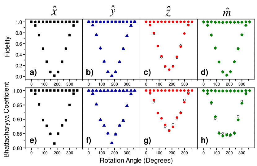
Figure 5: Summary of of the experimentally measured fidelity and the Bhattacharyya Coefficient for a wide range of unitaries. Panels a)–d) show the fidelity analysis results for unitary rotations about $\hat{x}$, $\hat{y}$, $\hat{z}$, and $\hat{m}$ axes as functions of rotation angle. The coloured data points are the comparison between stage I and stage III, and stage I and stage II. The open circles show the theoretical comparison which takes the state from stage I and applies theoretical unitaries. Panels e)–h) show the Bhattacharyya results comparing stage I and stage III, and stage I and stage II, in the coloured data points for each of the four axis, with the open circles being the theoretical comparison.

I.2 Fitting Son’s theory to experimental data as a test of Born’s rule

In our experiment, we place a bound on the degree of envariance. It has been shown that envariance can be used to derive Born’s rule zurek03.1 ; born26 . However, the derivation does not relate bounds on Born’s rule to bound on envariance. In order to do so, we explore a recently proposed extension of quantum mechanics by Son wonmin . Son’s theory generalizes Born’s rule, replacing the familiar power of 2 which relates wavefunctions to probabilities with a power of $n$. In this section, we summarize Son’s theory and use it to put a bound on $n$ using our experimental data.

We first consider measurements on a pair of qubits in the maximally entangled singlet state using standard quantum mechanics. We define measurement observables $\hat{a}=\vec{\alpha}\cdot\vec{\sigma_{1}}$ and $\hat{b}=\vec{\beta}\cdot\vec{\sigma_{2}}$ where $\vec{\alpha}$, $\vec{\beta}$ are unit vectors and $\vec{\sigma_{1}}$, $\vec{\sigma_{2}}$ are the Pauli matrices for the two qubits. The result of measurements $a$ and $b$ for qubits 1 and 2 respectively can take on the values $\pm 1$. The correlation function is defined by

$$E=\langle ab\rangle=P_{a=b}-P_{a\neq b},$$ (6)

where $P_{a=b}$ and $P_{a\neq b}$ are probabilities that $a=b$ and $a\neq b$ respectively. The correlation function only depends on the angle $2\theta$ between $\vec{\alpha}$ and $\vec{\beta}$ for the singlet state. From Born’s rule, we have the probability amplitudes $\psi_{a=b}$ and $\psi_{a\neq b}$ satisfy $P_{a=b}=|\psi_{a=b}|^{2}$ and $P_{a\neq b}=|\psi_{a\neq b}|^{2}$. Therefore, the correlation function in standard quantum mechanics is given by

$$E_{QM}(\theta)=|\psi_{a=b}|^{2}-|\psi_{a\neq b}|^{2}=-\cos 2\theta.$$ (7)

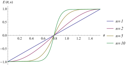
Figure 6: Generalized correlations for the singlet state as a function of $n$ using Son’s theory wonmin . The correlation as a function of $\theta$ is shown for $n=1$ (blue line), $n=2$ (purple line), $n=5$ (brown line) and $n=10$ (green line). The $n=2$ case corresponds to standard quantum mechanics.

We now consider Son’s theory, where Born’s rule is generalized to be $P_{a=b}=|\psi_{a=b}|^{n}$ and $P_{a\neq b}=|\psi_{a\neq b}|^{n}$, and the correlation function is thus,

$$E(\theta,n)=|\psi_{a=b}|^{n}-|\psi_{a\neq b}|^{n},$$ (8)

where standard quantum mechanics is the special case $E(\theta,2)=E_{QM}(\theta)$. As in standard quantum mechanics, Son assumed that the correlation function depends only on the angle between measurement settings. Son showed that the constraints $|\frac{\partial\psi_{a=b}}{\partial\theta}|^{2}+|\frac{\partial\psi_{a\neq b}}{\partial\theta}|^{2}\propto 1$ and $|\psi_{a=b}|^{n}+|\psi_{a\neq b}|^{n}=1$ and the boundary condition $E(0,n)=-1$ and $E(\frac{\pi}{2},n)=1$ are sufficient to solve for $E(\theta,n)$. See wonmin for further details on the deviation. Figure  6 shows $E(\theta,n)$ for different value $n$.

In the experiment, we rotated one qubit while leaving the other qubit unchanged during the stage II (See Figure  2) . If we use the same measurement basis on both qubits for that rotated state, we are effectively measuring the singlet state input with two measurement basis with angle $\theta$ apart. For example, we can choose the rotation axis and the measurement basis to be [Z,(D,A)], where the first qubit is rotated around Z axis, while measurements on the qubits are done in (D,A) basis. Since the rotation axis Z is orthogonal to the measurement basis (D,A), we could view the rotation of qubit as a rotation of the measurement basis in the D-A plane. For a rotation angle $\phi$, the angle between two measurement basis is given by $2\theta=\pi-|\pi-2\phi|$. We could derive prediction of $E(\phi,n)$ from Son’s theory, and test it with our data.

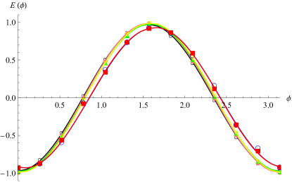
Figure 7: Correlation functions versus the rotation angle $\phi$. The experimental correlations are extracted from our data for the case where the rotation axis and the measurement basis are given by {[Z,(D,A)], [Z,(R,L)], [Y,(D,A)], [Y,(H,V)], [X,(R,L)], [X,(H,V)]} shown as {red squares, blue circles, green up triangles, yellow down triangles, black empty squares, pink diamonds} as a function of the rotation angle $\phi$. The best fit using Eq. 9 for each correlation is shown as a line whose colour matches the corresponding data points. These fits yield estimates for the value of $n$ of {2.04, 2.01, 2.00, 2.01, 2.01, 2.00}, respectively

Son’s derivation assumes a perfect singlet state which must be relaxed to obtain a comparison with experiment. For a realistic state, the correlation function will not necessarily depend only on $\theta$. In his derivation, Son additionally assumed $E(0,n)=-1$ and $E(\pi/2,n)=1$, i.e., perfect correlations, which are not experimentally achievable. To relax these assumptions, we consider the difference between two correlation functions measured for a general state $\rho$ and the ideal state $|\psi^{-}\rangle$, $E(\phi,n,\rho)$ and $E(\phi,n,|\psi^{-}\rangle)$ where $\phi$ is the rotation angle of one of the settings. For $n\approx 2$, we make the assumption that $E(\phi,n,\rho)-E(\phi,n,|\psi^{-}\rangle)\approx E(\phi,2,\rho)-E(\phi,2,|\psi^{-}\rangle)$. Thus for states close to the ideal singlet state and for $n$ close to 2, we have the relation:

$$E(\phi,n,\rho)\approx E(\phi,n,|\psi^{-}\rangle)+E(\phi,2,\rho)-E(\phi,2,|\psi^{-}\rangle).$$ (9)

We calculated $E(\phi,2,\rho)$ and $E(\phi,2,|\psi^{-}\rangle)$ from standard quantum mechanics, and use Son’s theory to calculate $E(\phi,n,|\psi^{-}\rangle)$. For a given set of data $E_{exp}(\phi_{i})$, we find $\rho$ and $n$ to minimize the objective function $L=\Sigma_{i}[E(\phi_{i},n,\rho)-E_{exp}(\phi_{i})]^{2}/[\delta E_{exp}(\phi_{i})]^{2}$, where $\delta E_{exp}(\phi_{i})$ is the standard deviation of correlation function $E_{exp}(\phi_{i})$ predicted assuming Poissonian count statistics. Figure 7 shows the results of fitting the correlation functions for 6 sets of data. From this, we extracted $n=2.04,2.01,2.00,2.01,2.01,2.00$; averaging these results and using their standard deviation to estimate the uncertainty yields $n=2.01\pm 0.02$ in good agreement with Born’s rule where $n=2$.

References

- (1) W. H. Zurek, Phys. Rev. A 71, 052105 (2005)
- (2) W. H. Zurek, Phys. Rev. Lett. 90, 120404 (2003)
- (3) W. H. Zurek, Rev. Mod. Phys. 75, 715 (2003)
- (4) R. Jozsa, J. Mod. Opt. 41, 2315 (1994).
- (5) A. Bhattacharyya , Bulletin of the Calcutta Mathematical Society 35, 99 (1943).
- (6) W.H. Zurek, Physics Today 44(10), 36 (1991).
- (7) M. Schlosshauer, Rev. Mod. Phys. 76, 1267-1305 (2004)
- (8) L. Landau, Z. Phys. 45, 430 (1927).
- (9) M. A. Nielsen and I. L. Chuang, Quantum Computation and Quantum Information, (Cambridge University Press, Cambridge, England, 2000).
- (10) M. Born, Z. Phys. 38, 803 (1926).
- (11) M. Schlosshauer and A. Fine, Found. Phys. 35, 197 (2005).
- (12) U. Mohrhoff, Int. J. Quantum Inf. 2, 221 (2004)
- (13) H. Barnum, e-print arXiv:quant-ph/0312150 (2008)
- (14) T. Kim, M. Fiorentino, and F. N. C. Wong, Phys. Rev. A 73, 012316 (2006).
- (15) A. Fedrizzi, T. Herbst, A. Poppe, T. Jennewein, and A. Zeilinger, Optics Express 15, 15377 (2007).
- (16) D. N. Biggerstaff, et al., Phys. Rev. Lett. 103, 240504 (2009).
- (17) M. Ježek, J. Fiurášek, and Z. Hradil, Phys. Rev. A 68, 012305 (2003).
- (18) W. Son, e-print arXiv:quant-ph/1401.1012 (2014).