MIFPA-14-24      Imperial/TP/14/KSS/02

We present a construction employing a type IIA supergravity and 3-form flux background together with an NS5-brane that localises massless gravity near the 5-brane worldvolume. The nonsingular underlying type IIA solution is a lift to 10D of the vacuum solution of the 6D Salam-Sezgin model and has a hyperbolic ${\cal H}^{(2,2)}\times S^{1}$ structure in the lifting dimensions. A fully back-reacted solution including the NS5-brane is constructed by recognising the 10D Salam-Sezgin vacuum solution as a “brane resolved through transgression.” The background hyperbolic structure plays a key rôle in generating a mass gap in the spectrum of the transverse-space wave operator, which gives rise to the localisation of gravity on the 6D NS5-brane worldvolume, or, equally, in a further compactification to 4D. Also key to the successful localisation of gravity is the specific form of the corresponding transverse wavefunction Schrödinger problem, which asymptotically involves a $V=-1/(4\rho^{2})$ potential, where $\rho$ is the transverse-space radius, and for which the NS5-brane source gives rise to a specific choice of self-adjoint extension for the transverse wave operator. The corresponding boundary condition as $\rho\to 0$ ensures the masslessness of gravity in the effective braneworld theory. Above the mass gap, there is a continuum of massive states which give rise to small corrections to Newton’s law.

1 Introduction: the problem of localising gravity on a brane

The problem of how to localise gravity on a submanifold of a higher-dimensional spacetime has been a key concern for cosmological braneworld models since the beginnings of the subject [1]. With compact extra dimensions, this is not a main concern, because there is a natural eigenvalue gap between a zero-mode of the Laplacian for the transverse dimensions and the first excited state, giving a corresponding mass gap in the effective 4D theory spectrum between massless 4D gravitational modes and the lowest lying massive modes. With noncompact extra dimensions, however, the problem that arises in principal is to avoid having a continuum of massive states ranging down all the way to those corresponding to massless 4D gravity.

An approach to the localisation of gravity on a 4D subsurface of an infinite higher-dimensional spacetime was given in [2, 3], joining segments of $\hbox{AdS}_{5}$ with the junction providing a delta-function source to the Einstein equations which gives rise to a normalisable bound state in the corresponding effective Schrödinger problem. Similar constructions involving excisions of spacetime were made, for example in [4]. A problem with such constructions, however, is to realise the delta-function source as a natural brane construct in string or M-theory. An embedding of the 5D ${{\mathbb{Z}}}_{2}$ symmetric construction of Ref. [2] was given in [5], but lifting the 5D realisation up to 10D proved to involve a singularity with no clear brane or orbifold interpretation, located at the lift of the ${{\mathbb{Z}}}_{2}$ reflection point [6].

An analysis of the difficulties of realising lower-dimensional gravity, massless or massive, on a subsurface of an infinite higher-dimensional spacetime was given in Ref.  [7]. For string constructions with asymptotically maximally-symmetric spacetimes (de Sitter, Poincaré, or anti-de Sitter), it proves to be difficult to obtain the peak in the warp factor for the 4D subspace that is needed in order to give rise to the localising bound state.

Another theme in the study of supergravity theories which has been somewhat explored but not widely applied is the existence of supergravity models with noncompact gauge symmetries (see, for example, [8]). Such gaugings may elegantly be obtained using the embedding-tensor formalism [9]. Models with gauged noncompact group symmetries of this sort manage to have a purely positive-energy spectrum thanks to the nonlinear realisation of the noncompact symmetry on appropriate sets of scalar fields, acting on prefix factors of positive-energy kinetic terms, with linear realisation only on a compact subgroup of the gauged symmetry. One reason that few proposed physical applications of higher-dimensional models with noncompact gauge symmetries have been made, however, is the generally continuous spectrum of eigenstates in the space transverse to the lower-dimensional spacetime. The corresponding continuous spectrum of effective-theory massive states can prevent the effective localisation of lower-dimensional gravity, unless somehow a mass gap can be arranged below the edge of the continuous spectrum.

In this paper, we combine these two developments to provide a construction that localises gravity on a subspace of a background spacetime arising from just such a noncompact gauged supergravity. Instead of a simple patching of slices of the background spacetime, however, our construction employs a natural object in string or M-theory: an NS5-brane. This is one of the fundamental brane objects arising in 11D M-theory [10], and it gives rise, upon “vertical” dimensional reduction [11], to the NS5-brane of type IIA supergravity.

The construction is ultimately based upon a 6D model with R-symmetry gauging obtained by Salam and Sezgin in 1984 [12]. This model has the unusual property of having a scalar field with a positive potential, as opposed to the negative or indefinite sign potentials arising in models with gauged compact symmetries. Although the Salam-Sezgin model does not admit a maximally symmetric 6D spacetime solution, the positive scalar potential does allow for a solution combining an $S^{2}$ subspace with $U(1)$ magnetic monopole flux and with flat 4D Minkowski space. The link between the Salam-Sezgin model and supergravities related to string theory is given by its embedding into 10D type IIA supergravity by a lift on the noncompact space ${\cal H}^{(2,2)}$ [13]. When viewed as a 7D supergravity theory, the full theory obtained via ${\cal H}^{(2,2)}$ reduction from 10D has a gauged ${\rm SO}(2,2)$ symmetry, positive-energy kinetic terms for all fields and 9 scalar fields with a positive-definite potential generalising that of the Salam-Sezgin model (which can then be obtained by a consistent truncation of the ${\rm SO}(2,2)$ invariant theory). If desired, the construction can be extended to an 11D embedding by the inclusion of an additional lift on a further spatial $S^{1}$.

In Section 2, we begin by presenting the details of the embedding of the Salam-Sezgin 6D $S^{2}\times{{\mathbb{R}}}^{4}$ “vacuum” solution into a 10D type IIA supergravity solution via a Kaluza-Klein lift on ${\cal H}^{(2,2)}$. This then sets the stage in Section 3 for an initial analysis of gravitational fluctuations about the Salam-Sezgin background, and for a discussion of normalisable candidate bound states that could localise gravity in a lower-dimensional subspacetime. For spin-two excitations, a simplifying feature of such analysis is that one needs only to study the scalar wave equation in the space transverse to the lower-dimensional spacetime [14, 7]. The only such wavefunction that can explicitly be given in terms of standard functions turns out to be the zero-eigenvalue eigenfunction $\xi_{0}$ of the transverse wave operator. Gravitational fluctuations with this transverse wavefunction structure are massless from the point of view of the lower-dimensional physics. However, the wavefunction $\xi_{0}$ has a logarithmic asymptotic behaviour as one approaches the “waist” ($\rho=0$ in the radial coordinate) of the ${\cal H}^{(2,2)}$ space, as distinct from the non-singular structure of the underlying Salam-Sezgin vacuum. This implies the need for a source at $\rho=0$ in the fluctuation wave equation.

Preserving the eight-supercharge unbroken supersymmetry of the vacuum Salam-Sezgin solution points to a NS5-brane as the relevant inclusion, as analysed in Section 4, which then proceeds on to a main result: the fully back-reacted solution generalising the Salam-Sezgin vacuum background by the inclusion of an NS5-brane. The key to this construction is recognition of the nonsingular vacuum Salam-Sezgin solution, when reduced from 10D to 9D by compactification on the NS5-brane “waist” coordinate $\psi$, as an instance of a “brane resolved by transgression” in the fashion of Ref. [15].

In Section 5, the needed NS5-brane worldvolume source action is included in the field equations, yielding, firstly, the relation between the NS5-brane tension $T$ and the integration constant $k$ found for the bulk solution inclusion of the NS5-brane, and secondly, the boundary conditions for transverse fluctuation wavefunctions that are required by the NS5-brane source. This analysis is surprisingly subtle, especially concerning the question of self-adjointness of the transverse wave operator: the corresponding Schrödinger problem for the transverse wavefunction involves, asymptotically as $\rho\to 0$, a potential $V=-1/(4\rho^{2})$, which has represented a continuing puzzle in quantum mechanics since the 1950’s [16, 17, 18, 19]. Analysis of the NS5-brane source action’s implications for the asymptotic $\rho\to 0$ structure of the transverse wavefunction, with careful regulation of the corresponding source delta function, selects just one transverse bound state. This is the zero mode $\xi_{0}$, which happily remains exactly the same as in the preliminary fluctuation analysis about the Salam-Sezgin vacuum solution given in Section 2. This yields massless gravity in the lower-dimensional braneworld. Moreover, as one moves away from the $\rho=0$ “waist” of the ${\cal H}^{(2,2)}$ space, the Schrödinger potential rises to a positive value $(1+k)$, depending on the strength $k$ of the NS5-brane. This gives rise to a $(1+k)g^{2}$ gap in the lower-dimensional braneworld $(\hbox{mass})^{2}$ eigenvalues between the massless states and the edge of the continuum massive spectrum, where $g$ is the $(\hbox{length})^{-1}$ dimensional parameter characterising the scale of the ${\cal H}^{(2,2)}$ hyperbolic geometry.

The lower-dimensional effective braneworld gravity arising from this construction is initially six-dimensional, corresponding to the worldvolume dimension of the NS5-brane. Of these six worldvolume dimensions, the “waist” coordinate $\psi$ is naturally compactified. Another worldvolume coordinate, $y$, may be chosen to be compactified on $S^{1}$, or can be used in an $S^{1}/{{\mathbb{Z}}}_{2}$ Hořava-Witten [20] type construction in order to produce a 4D chiral theory, with attendant matter fields as needed to cancel anomaly inflow [21, 22]. The 4D effective gravity is next analysed. Normalisation of the $\xi_{0}$ bound-state transverse wavefunction is carried out explicitly in Section 6 and a preliminary consideration of corrections to 4D Newtonian gravity arising from the continuum of massive states is given in Section 7. The paper concludes in Section 8 with a consideration of open problems and the realisation of our construction in string theory.

2 Salam-Sezgin theory and its embedding in ${\cal H}^{(2,2)}$

The bosonic sector of the six-dimensional Salam-Sezgin theory is described by the Lagrangian

$$\bar{\cal L}_{6}=\bar{R}\,{\bar{*}\hbox to0.0pt{1\hss}\mkern 4.0mu{\rm l}}-{\textstyle{{\scriptstyle 1}\over{\scriptstyle 4}}}{\bar{*}d\bar{\phi}}\wedge d\bar{\phi}-{\textstyle{{\scriptstyle 1}\over{\scriptstyle 2}}}e^{{\textstyle{{\scriptstyle 1}\over{\scriptstyle 2}}}\bar{\phi}}\,{\bar{*}\bar{F}_{{\scriptscriptstyle(2)}}}\wedge\bar{F}_{{\scriptscriptstyle(2)}}-{\textstyle{{\scriptstyle 1}\over{\scriptstyle 2}}}e^{\bar{\phi}}\,{\bar{*}\bar{H}_{{\scriptscriptstyle(3)}}}\wedge\bar{H}_{{\scriptscriptstyle(3)}}-8\bar{g}^{2}\,e^{-{\textstyle{{\scriptstyle 1}\over{\scriptstyle 2}}}\bar{\phi}}\,{\bar{*}\hbox to0.0pt{1\hss}\mkern 4.0mu{\rm l}}\,,$$ (2.1)

where $d\bar{H}_{{\scriptscriptstyle(3)}}={\textstyle{{\scriptstyle 1}\over{\scriptstyle 2}}}\bar{F}_{2}\wedge\bar{F}_{{\scriptscriptstyle(2)}}$ and $\bar{F}_{2}=d\bar{A}_{{\scriptscriptstyle(1)}}$. (We put a bar on all quantities in the six-dimensional theory.) It was shown in [13] that the Salam-Sezgin theory can be embedded in the ten-dimensional type I supergravity theory whose bosonic Lagrangian can be taken to be

$${\cal L}_{10}=R\,{*\hbox to0.0pt{1\hss}\mkern 4.0mu{\rm l}}-{\textstyle{{\scriptstyle 1}\over{\scriptstyle 2}}}{*d\phi}\wedge d\phi-{\textstyle{{\scriptstyle 1}\over{\scriptstyle 2}}}e^{-\phi}{*F_{3}}\wedge F_{{\scriptscriptstyle(3)}}\,,$$ (2.2)

via a consistent dimensional reduction on ${{\mathbb{R}}}$ times the three-dimensional hyperbolic space ${\cal H}^{(2,2)}$. This space can be defined as the surface $X_{1}^{2}+X_{2}^{2}-X_{3}^{2}-X_{4}^{2}=1$ embedded in the Euclidean space ${{\mathbb{E}}}^{4}$, with the natural metric inherited as the restriction of $ds_{\rm Euclidean}^{2}=dX_{1}^{2}+dX_{2}^{2}+dX_{3}^{2}+dX_{4}^{2}$ to this surface. Its isometry group is $U(1)\times U(1)$, which is the intersection of the ${\rm O}(2,2)$ symmetry of the embedding condition and the ${\rm O}(4)$ symmetry of the Euclidean metric on ${{\mathbb{E}}}^{4}$. It was shown in [13] that the metric on ${\cal H}^{(2,2)}$ can be written as

$$ds_{3}^{2}=\cosh 2\rho\,d\rho^{2}+\cosh^{2}\rho\,d\alpha^{2}+\sinh^{2}\rho\,d\beta^{2}\,,$$ (2.3)

where $\rho\geq 0$ and $0\leq\alpha<2\pi$, $0\leq\beta<2\pi$. It will be more convenient for our purposes to introduce coordinates $\psi\in[0,4\pi)$ and $\chi\in[0,2\pi)$ in place of $\alpha$ and $\beta$, defined by

$$\psi=\alpha+\beta\,,\qquad\chi=\alpha-\beta\,.$$ (2.4)

In terms of these, the embedding of the Salam-Sezgin theory in ten-dimensional type I supergravity that was constructed in [13] is given by

$$ds_{10}^{2} = (\cosh 2\rho)^{1/4}\,\Big{[}e^{-{\textstyle{{\scriptstyle 1}\over{\scriptstyle 4}}}\bar{\phi}}\,d\bar{s}_{6}^{2}+e^{{\textstyle{{\scriptstyle 1}\over{\scriptstyle 4}}}\bar{\phi}}\,dy^{2}+{\textstyle{{\scriptstyle 1}\over{\scriptstyle 2}}}\bar{g}^{-2}\,e^{{\textstyle{{\scriptstyle 1}\over{\scriptstyle 4}}}\bar{\phi}}\,\Big{(}d\rho^{2}$$ (2.6)

$$+{\textstyle{{\scriptstyle 1}\over{\scriptstyle 4}}}[d\psi+{\hbox{sech}}2\rho(d\chi-2\bar{g}\bar{A})]^{2}+{\textstyle{{\scriptstyle 1}\over{\scriptstyle 4}}}(\tanh 2\rho)^{2}\,(d\chi-2\bar{g}\bar{A})^{2}\Big{)}\Big{]}\,,$$

$$F_{{\scriptscriptstyle(3)}} = \bar{H}_{{\scriptscriptstyle(3)}}-{\sinh 2\rho\over 4\bar{g}^{2}(\cosh 2\rho)^{2}}\,d\rho\wedge d\psi\wedge(d\chi-2\bar{g}\bar{A}_{{\scriptscriptstyle(1)}})$$ (2.8)

$$+{1\over 4\bar{g}\cosh 2\rho}\,\bar{F}_{2}\wedge[d\psi+\cosh 2\rho\,(d\chi-2\bar{g}\bar{A}_{{\scriptscriptstyle(1)}})]\,,$$

$$e^{\phi} = (\cosh 2\rho)^{-1/2}\,e^{-{\textstyle{{\scriptstyle 1}\over{\scriptstyle 2}}}\bar{\phi}}\,.$$ (2.9)

For the present, our focus will be on the remarkable (Minkowski)${}_{4}\times S^{2}$ vacuum solution of the Salam-Segin theory [12], which is given by

$$d\bar{s}_{6}^{2} = dx^{\mu}dx^{\nu}\eta_{\mu\nu}+{1\over 8\bar{g}^{2}}\,(d\theta^{2}+\sin^{2}\theta d\varphi^{2})\,,$$ (2.10)

$$\bar{A}_{{\scriptscriptstyle(1)}} = -{1\over 2\bar{g}}\,\cos\theta\,d\varphi\,,\qquad\bar{H}_{{\scriptscriptstyle(3)}}=0\,,\qquad\bar{\phi}=0\,.$$ (2.11)

The lift of this solution to ten dimensions, using (2.9), was given in [13]. As noted there, the solution is more elegantly written in the ten-dimensional string-frame metric $ds^{2}_{\rm str}$, related to the Einstein-frame metric $ds_{10}^{2}$ by

$$ds^{2}_{10\,\rm str}=e^{{\textstyle{{\scriptstyle 1}\over{\scriptstyle 2}}}\phi}\,ds_{10}^{2}\,.$$ (2.12)

After making the coordinate transformation (2.4) the lifted Salam-Sezgin vacuum is given by [13] 

$$ds^{2}_{10\,\rm str} = dx^{\mu}dx^{\nu}\eta_{\mu\nu}+dy^{2}+{1\over 4g^{2}}\,[d\psi+{\hbox{sech}}2\rho\,(d\chi+\cos\theta\,d\varphi)]^{2}+{1\over g^{2}}\,{\hbox{sech}}2\rho\,ds^{2}_{\rm{\scriptscriptstyle EH}}\,,$$ (2.14)

$$e^{\phi} = ({\hbox{sech}}2\rho)^{1/2}\,,\qquad A_{{\scriptscriptstyle(2)}}={1\over 4g^{2}}\,[d\chi+{\hbox{sech}}2\rho\,d\psi]\wedge(d\chi+\cos\theta\,d\varphi)\,,$$ (2.15)

where

$$ds^{2}_{\rm{\scriptscriptstyle EH}}=\cosh 2\rho\,d\rho^{2}+{(\sinh 2\rho)^{2}\over 4\cosh 2\rho}\,(d\chi+\cos\theta\,d\varphi)^{2}+{\textstyle{{\scriptstyle 1}\over{\scriptstyle 4}}}\cosh 2\rho\,(d\theta^{2}+\sin^{2}\theta\,d\varphi^{2})\,.$$ (2.16)

We now observe that if we make the coordinate transformation $\cosh 2\rho=r^{2}$, the metric $ds^{2}_{\rm{\scriptscriptstyle EH}}$ becomes

$$ds^{2}_{\rm{\scriptscriptstyle EH}}=\Big{(}1-{1\over r^{4}}\Big{)}^{-1}\,dr^{2}+{\textstyle{{\scriptstyle 1}\over{\scriptstyle 4}}}r^{2}\,\Big{(}1-{1\over r^{4}}\Big{)}\,(d\chi+\cos\theta\,d\varphi)^{2}+{\textstyle{{\scriptstyle 1}\over{\scriptstyle 4}}}r^{2}\,(d\theta^{2}+\sin^{2}\theta\,d\varphi^{2})\,.$$ (2.17)

This can be recognised as the Eguchi-Hanson metric, with unit scale parameter [23]. Recalling that the $\chi$ coordinate has period $2\pi$, one sees from (2.16) that at large distance the space approaches ${{\mathbb{R}}}^{4}/{{\mathbb{Z}}}_{2}$ [24]. On the other hand, as $\rho$ goes to zero, $\rho$ and $\chi$ become like plane polar coordinates in the neighbourhood of the origin, so the space approaches ${{\mathbb{R}}}^{2}\times S^{2}$ there.

The Salam-Sezgin (Minkowski)${}_{4}\times S^{2}$ vacuum is supersymmetric [12] in six dimensions, and hence it lifts to a supersymmetric solution in ten dimensions. The general reduction of the fermions was discussed also in [13]. For our present purposes, it is useful just to exhibit the Killing spinors of the lifted Salam-Sezgin vacuum (2.15). These are most elegantly expressed in the string frame also, wherein the ten-dimensional supersymmetry transformation rules take the form

$$\delta\psi_{M}=\nabla_{M}\,{\epsilon}-{\textstyle{{\scriptstyle 1}\over{\scriptstyle 8}}}F_{MNP}\,\Gamma^{NP}\,\Gamma_{11}\,{\epsilon}\,,\qquad\delta\lambda=\Gamma^{M}\partial_{M}\phi\,{\epsilon}-{\textstyle{{\scriptstyle 1}\over{\scriptstyle 12}}}F_{MNP}\,\Gamma^{MNP}\,\Gamma_{11}\,{\epsilon}\,.$$ (2.18)

We shall give a more detailed discussion of the derivation of the Killing spinors later, when we consider a modification of the ten-dimensional lift of the Salam-Sezgin vacuum in which a singular NS5-brane is introduced. For now we shall just present the result for the lifted Salam-Sezgin vacuum itself. We find that there exist eight Killing spinors, which are given by

$${\epsilon}=e^{-{\textstyle{{\scriptstyle 1}\over{\scriptstyle 2}}}\chi\,\Gamma_{89}}\,\eta\,,$$ (2.19)

where $\eta$ is any constant spinor satisfying the two projection conditions

$$\Gamma_{11}\,\eta=-\eta\,,\qquad\Gamma_{67}\eta=\Gamma_{89}\,\eta\,.$$ (2.20)

Here, the 6, 7, 8 and 9 vielbein indices on the gamma matrices refer to the four directions in the Eguchi-Hanson transverse space, with

$$\hat{e}^{6} = {\textstyle{{\scriptstyle 1}\over{\scriptstyle 2}}}\sinh 2\rho\,(\cosh 2\rho)^{-1/2}\,(d\chi+\cos\theta\,d\varphi)\,,\qquad\hat{e}^{7}=(\cosh 2\rho)^{1/2}\,d\rho\,,$$ (2.21)

$$\hat{e}^{8} = {\textstyle{{\scriptstyle 1}\over{\scriptstyle 2}}}(\cosh 2\rho)^{1/2}\,d\theta\,,\qquad\hat{e}^{9}={\textstyle{{\scriptstyle 1}\over{\scriptstyle 2}}}(\cosh 2\rho)^{1/2}\,\sin\theta\,d\varphi\,,$$ (2.22)

and $ds^{2}_{\rm{\scriptscriptstyle EH}}=\sum_{i=6}^{9}\hat{e}_{i}^{2}$.

3 Bound states and mass gaps

Now consider gravitational fluctuations around the Salam-Sezgin background, considered from a braneworld four-dimensional perspective. General studies [14, 7] of the fluctuation problem about supergravity backgrounds start with an ansatz replacing the 4D metric $\eta_{\mu\nu}$ by $\eta_{\mu\nu}+h_{\mu\nu}(x,z)$ where $x^{\mu}$ are the 4D coordinates and $z^{n}=(y,\psi,\theta,\varphi,\chi,\rho)$ are the six “transverse” coordinates. One notes from the Salam-Sezgin background solution (2.15) that, of these, the five coordinates $(y,\psi,\theta,\varphi,\chi)$ all refer to naturally compact directions, while $\rho$ is the non-compact “radius”. The fluctuation problem for $h_{\mu\nu}(x,z)$ can be treated by separation of variables. A full expansion of the fluctuations in the ten-dimensional theory would involve introducing harmonic eigenfunctions for the dependences on the five compact coordinates as well as the non-compact $\rho$ coordinate. However, for a study of the lowest-lying fluctuation states, one may simplify the problem by availing oneself of a consistent truncation to the sector independent of $y,\psi,\theta,\varphi\ \&\,\chi$: this amounts to considering only S-wave, i.e. singlet, states with respect to the corresponding background symmetries (i.e. $({\rm U}(1))^{3}$ for $y$, $\psi$ and $\chi$, and ${\rm SO}(3)$ for $\theta$ and $\varphi$). The essential remaining dependence is then on the non-compact coordinate $\rho$.

Accordingly, we posit an expansion

$$h_{\mu\nu}(x,\rho)=\sum_{i}h_{\mu\nu}^{(\lambda_{i})}(x)\xi_{\lambda_{i}}(\rho)+\int_{\Lambda_{\mbox{\scriptsize edge}}}^{\infty}d\lambda\,h_{\mu\nu}^{(\lambda)}(x)\xi_{\lambda}(\rho)\,,$$ (3.1)

where the $\xi_{\lambda_{i}}$ are discrete states and the $\xi_{\lambda}$ are continuum states for eigenvalues $\lambda$ starting from some lower value $\Lambda_{\mbox{\scriptsize edge}}$ at the edge of the continuous spectrum. Limiting attention to linearised 4D gravitational fluctuations in $h_{\mu\nu}(x)$ about the Salam-Sezgin background, we may focus on pure spin-two fluctuations with $\eta^{\mu\nu}h_{\mu\nu}(x)=0$ and we may also impose the gauge conditions $\partial^{\mu}h_{\mu\nu}(x)=0$. The analysis of [7] then shows that the gravitational fluctuations must solve a scalar wave equation in the full ten-dimensional spacetime

$$\square_{(10)}h_{\mu\nu}(x,z)=0\,,$$ (3.2)

where the 10D wave operator splits up as

$$\square_{(10)}=H_{{\scriptscriptstyle\rm SS}}^{\frac{1}{4}}(\square_{(4)}+g^{2}\triangle_{y,\psi,\theta,\varphi,\chi}+g^{2}\triangle_{\mbox{\scriptsize rad}})\,,$$ (3.3)

where

$$H_{{\scriptscriptstyle\rm SS}}=(\cosh 2\rho)^{-1}$$ (3.4)

is the Salam-Sezgin warp function, $\square_{(4)}$ is the 4D d’Alembertian, $\triangle_{y,\psi,\theta,\varphi,\chi}$ is the Laplacian for the five compact directions $(y,\psi,\theta,\varphi,\chi)$ (which will have zero eigenvalue for our S-wave treatment) and

$$\triangle_{\mbox{\scriptsize rad}}={\partial^{2}\over\partial\rho^{2}}+{2\over\tanh(2\rho)}{\partial\over\partial\rho}\,.$$ (3.5)

Solutions to (3.2) in ten dimensions will then give rise to 4D solutions with $(\hbox{mass})^{2}$ values given by the $\triangle_{\mbox{\scriptsize rad}}$ eigenvalue $\lambda$:

$$\triangle_{\mbox{\scriptsize rad}}\xi_{\lambda}(\rho) = -\lambda\xi_{\lambda}(\rho)\,,$$ (3.6)

$$\square_{(4)}h_{\mu\nu}^{\lambda}(x) = m^{2}h_{\mu\nu}^{\lambda}(x)\,,$$ (3.7)

$$m^{2} = g^{2}\lambda\,.$$ (3.8)

3.1 The Schrödinger equation for $\triangle_{\mbox{\scriptsize rad}}$ eigenfunctions

One can rewrite the $\triangle_{\mbox{\scriptsize rad}}$ eigenvalue problem as a Schrödinger equation by making the rescaling

$$\Psi_{\lambda}=\sqrt{\sinh(2\rho)}\xi_{\lambda}\,,$$ (3.9)

thereby eliminating the first-derivative term from the eigenfunction equation, which then takes the Schrödinger-equation form

$$-{d^{2}\Psi_{\lambda}\over d\rho^{2}}+V(\rho)\Psi_{\lambda}=\lambda\Psi_{\lambda}\,,$$ (3.10)

where the potential is

$$V(\rho)=2-{1\over\tanh^{2}(2\rho)}\,.$$ (3.11)

The Schrödinger equation potential (3.11) asymptotes to the value 1 for large $\rho$. In this large-$\rho$ limit, the Schrödinger equation becomes

$${d^{2}\Psi_{\lambda}\over d\rho^{2}}+4e^{-4\rho}\Psi_{\lambda}+(\lambda-1)\Psi_{\lambda}=0\,,$$ (3.12)

giving scattering-state solutions for $\lambda>1$:

$$\Psi_{\lambda}(\rho)\sim\left(A_{\lambda}e^{i\sqrt{\lambda-1}\rho}+B_{\lambda}e^{-i\sqrt{\lambda-1}\rho}\right)\quad\text{ for large $\rho$}\,,$$ (3.13)

while for $\lambda<1$ one can have $L^{2}$ normalizable candidate bound states. Recalling the $\rho$ dependence of the measure $\sqrt{-g_{(10)}}\sim(\cosh(2\rho))^{\frac{1}{4}}\sinh(2\rho)$, one finds for large $\rho$ that

$$\int_{\rho_{1}\gg 1}^{\infty}|\Psi_{\lambda}(\rho)|^{2}d\rho<\infty\Rightarrow\Psi_{\lambda}\sim B_{\lambda}e^{-\sqrt{1-\lambda}\rho}\quad\text{for }\lambda<1\,.$$ (3.14)

It follows that for $\lambda<1$, we have candidate bound states of the transverse $\triangle_{\mbox{\scriptsize rad}}$ system. We shall need to discover how to fix the value of $\lambda$. Clearly of particular interest will be the value zero, which corresponds to massless gravity in four dimensions.

Before analysing the transverse bound-state spectrum, we need to consider the norm that is to be used in considering the normalizability of the transverse wavefunction $\xi(\rho)$. In fact, for the rescaled wavefunction (3.9), the trivial $L^{2}$ norm is the correct one. One may see this by starting from the 10D type IIA action with Einstein-frame integration over $\int d^{10}x\sqrt{g_{{{\scriptscriptstyle(10)}}\,\rm ein}}$. With the $\eta_{\mu\nu}\rightarrow\eta_{\mu\nu}+h_{\mu\nu}(x,\rho)$ ansatz for the 4D gravitational fluctuations, one obtains the correct norm measure by collecting the $\rho$-dependent terms multiplying the 4D gravitational kinetic terms. In the quadratic terms of the 4D effective action, up to a constant factor of $\frac{1}{16g^{5}}$, one has $|\xi(\rho)|^{2}$ from the two $h_{\mu\nu}$ fields, multiplied by $H_{{\scriptscriptstyle\rm SS}}\sinh 2\rho\cosh 2\rho\sqrt{g_{{{\scriptscriptstyle(2)}}}}$ and then integrated over the six dimensions transverse to the 4D space, where $\sqrt{g_{{{\scriptscriptstyle(2)}}}}$ is the standard 2-sphere metric density. The $\rho$-dependent terms combine to give simply $\sinh 2\rho$. Consequently, after the wavefunction rescaling in (3.9), the correct norm for the transverse $\rho$-dependent wavefunction is simply

$$||\Psi||^{2}=\int d\rho|\Psi|^{2}\,.$$ (3.15)

3.2 The zero-mass candidate bound state

The general behaviour of candidate $\Psi_{\lambda}$ eigenfunctions cannot be given in terms of standard functions, but for $\lambda=0$ the Schrödinger equation happily can be solved exactly, giving the normalised result

$$\Psi_{0}(\rho) = \frac{2\sqrt{3}}{\pi}\sqrt{\sinh(2\rho)}\xi_{0}(\rho)\,,$$ (3.16)

$$\xi_{0}(\rho) = \log(\tanh\rho)\,.$$ (3.17)

Sketching the zero-mode wavefunction (3.16) and the potential (3.11) together, we have the picture shown in Figure 1:

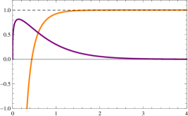
Figure 1: The normalizable zero-mode $\Psi_{0}$ and the ${\cal H}^{(2,2)}$ Schrödinger equation potential,
 limiting to the value 1 as $\rho\to\infty$.

The $(y,\psi,\theta,\varphi,\chi)$ coordinates correspond to a compact $T^{2}\times S^{2}\times S^{1}$ space on which one may make a standard Kaluza-Klein dimensional reduction. Note that $\chi$ is a coordinate corresponding to collapsing curves as one takes the limit $\rho\rightarrow 0$: the $\rho,\chi$ submanifold simply tends to ${{\mathbb{R}}}^{2}$ in this limit; we will come back to this point in the next section. All of the other compact coordinates correspond to non-collapsing curves and there is no subtlety in restricting attention to fields independent of $y$, $\psi$, $\theta$ and $\varphi$ on $T^{2}\times S^{2}$. Provided one has reason to specify the normalizable $\lambda=0$ wavefunction as the remaining part of the $h_{\mu\nu}(x,\rho)$ field dependence on the coordinates transverse to the 4D subspace, this will concentrate the gravitational fluctuations in the region closely surrounding the 4D subspace and will give rise to massless 4D effective gravity. It remains now to justify why this zero mode is in fact the correct transverse wavefunction.

4 Salam-Sezgin background with an NS5-brane inclusion

In the preceding section, we found an attractive zero-mode candidate for the gravitational fluctuation wavefunction in the space transverse to our 4D spacetime. There are, however, two linked aspects of this zero-mode wavefunction that require us to expand our consideration of background type IIA supergravity solutions in which the 4D gravity-localising subspace may be embedded. Although the Salam-Sezgin background (2.15) is itself a completely smooth solution of type IIA supergravity, the $\xi_{0}$ zero-mode (3.17) diverges in the limit as $\rho\rightarrow 0$. Moreover, as we shall see in detail later, this transverse wavefunction does not, strictly speaking, yield a true solution of type IIA supergravity: it requires a source at $\rho=0$ (just as the $1/r$ potential requires a source in the 3D Laplace equation). This situation is not in itself any more disturbing than the need, strictly speaking, for a source for the M2 brane [25], or for essentially any of the classic string or M-theory brane solutions. But the question before us here is: a source for what? A number of hints can be found in the Salam-Sezgin background solution (2.15) and in the logarithmic character of the $\xi_{0}$ zero-mode itself.

The $\log\rho$ behaviour of $\xi_{0}(\rho)$ as $\rho\rightarrow 0$ is a clear hint that this wavefunction belongs to a two-dimensional transverse space. The natural coordinate to accompany $\rho$ in this transverse 2-space is $\chi$, which together with $\rho$ comprises polar coordinates on ${{\mathbb{R}}}^{2}$, in the limit $\rho\rightarrow 0$, as mentioned above. If we are looking to modify the Salam-Sezgin solution by the inclusion of some kind of brane, the natural situation would be to have a flat subspace of the 10D solution as the worldvolume. Within the Salam-Sezgin background solution (2.15), in addition to the flat 4D coordinates $x^{\mu}$, the $T^{2}$ coordinates $y$ and $\psi$ are a natural pair of coordinates of further flat directions. So the suggestion is to consider $(x^{\mu},y,\psi)$ as world-volume coordinates, with $(\rho,\chi,\theta,\varphi)$ as coordinates transverse to a brane inclusion. This implies that one should look for a 5-brane inclusion, with $(x^{\mu},y,\psi)$ as the worldvolume coordinates. Of the transverse coordinates, we clearly want to focus on solutions depending only on $\rho$, and so we will not be exciting modes depending on $\theta$, $\varphi$ or $\chi$. As we have seen, however, $\chi$, together with $\rho$, form polar coordinates on ${{\mathbb{R}}}^{2}$ near $\rho=0$, and although we will not be considering functional dependence on $\chi$, care will be needed in treating it, since it is part of a suspected operative two-dimensional transverse space. The coordinates $(\theta$ and $\varphi$ parameterise an $S^{2}$ in the transverse space, on which we will be considering only S-wave, i.e. $S^{2}$-independent, solutions. The hints from the structure of the 10D Salam-Sezgin solution (2.15) therefore point towards the inclusion of a 5-brane smeared over the transverse $S^{2}$ directions, thus leaving $\rho$ and $\chi$ as the coordinates of the operative two-dimensional transverse space, in which a wave function logarithmic in $\rho$ would be natural.

The hints of 5-brane structure in the Salam-Sezgin solution were noted already in Reference [13], where the $\rho\to\infty$ asymptotic structure of the Salam-Sezgin background was identified with an NS5-brane geometry in ten dimensions, with two of the worldvolume coordinates (here $y$ and $\psi$) wrapped around a $T^{2}$ torus. This structure thus makes use of both the “diagonal” and “vertical” dimensional reduction arrangements outlined in Reference [11].

A further confirmation that an NS5-brane is the right kind of brane inclusion to consider comes from supersymmetry. We saw in (2.19) and (2.20) that the Salam-Sezgin background has eight unbroken supersymmetries. Supersymmetry preservation for a probe NS5-brane on this background follows from the requirement of $\kappa$-symmetry invariance. For a probe NS5-brane with worldvolume directions $(0,1,2,3,4,5)$ in the notation of Section 2, the corresponding requirement is [26]

$$\Gamma_{012345}\eta=\eta\,.$$ (4.1)

The appropriateness of an NS5-brane inclusion can then be seen by rewriting the second equation in (2.20) as

$$\Gamma_{6789}\eta=-\eta\,.$$ (4.2)

The first equation in (2.20) can be rewritten as

$$\Gamma_{012345}\Gamma_{6789}\eta=-\eta\,,$$ (4.3)

and so (4.2) and (4.3) together imply (4.1) already from the Salam-Sezgin supersymmetry conditions, resulting in no further diminution of unbroken supersymmetry arising from the inclusion of an NS5-brane: the eight unbroken Salam-Sezgin supersymmetries persist upon inclusion of an NS5-brane.

These considerations based on the structure of the Salam-Sezgin background geometry and probe-brane supersymmetry preservation indicate that the inclusion of an NS5-brane in the Salam-Sezgin geometry is the appropriate way to create an initially static background about which 4D massless gravitational fluctuations with a normalizable transverse wavefunction can exist. To complete the construction, however, we will need a fully back-reacted geometry including an NS5-brane. Constructing this solution is now our main task.

4.1 Lifted Salam-Sezgin vacuum and brane resolution by transgression

In order to show how an NS5-brane can be introduced, it is helpful first to perform a dimensional reduction to 9D of the ten-dimensional IIA theory, and of the lifted Salam-Sezgin vacuum, on a circle. Specifically, we shall reduce on the $\psi$ coordinate in (2.9) and (2.15), or, more precisely, on the rescaled dimensionful coordinate

$$w\equiv{1\over 2g}\,\psi.$$ (4.4)

It is convenient to use the string frames in ten and in nine dimensions, with the reduction ansatz

$$ds_{10\,\rm str}^{2}=d\tilde{s}_{9\,\rm str}^{2}+e^{\sqrt{2}\,\tilde{\phi}_{2}}\,(dw+\tilde{{\cal A}}_{{\scriptscriptstyle(1)}})^{2}\,,\qquad A_{{\scriptscriptstyle(2)}}=\tilde{A}_{{\scriptscriptstyle(2)}}+\tilde{A}_{{\scriptscriptstyle(1)}}\wedge dw\,.$$ (4.5)

(We put tildes on all nine-dimensional fields.) The dimensionally-reduced theory in nine dimensions, written now in the Einstein frame $d\tilde{s}_{9\,\rm ein}^{2}=e^{-2\phi/\sqrt{7}+\sqrt{2}\,\tilde{\phi}_{2}/7}\,d\tilde{s}_{9\,\rm str}^{2}$, is described by the Lagrangian

$$\tilde{\cal L}_{9}=\sqrt{-\tilde{g}}\,\Big{(}\tilde{R}-{\textstyle{{\scriptstyle 1}\over{\scriptstyle 2}}}(\partial\phi_{1})^{2}-{\textstyle{{\scriptstyle 1}\over{\scriptstyle 2}}}(\partial\tilde{\phi}_{2})^{2}-{\textstyle{{\scriptstyle 1}\over{\scriptstyle 12}}}\,e^{{\textstyle{{\scriptstyle 4}\over{\scriptstyle\sqrt{14}}}}\,\phi_{1}}\,\tilde{F}_{{\scriptscriptstyle(3)}}^{2}-{\textstyle{{\scriptstyle 1}\over{\scriptstyle 4}}}e^{{\textstyle{{\scriptstyle 2}\over{\scriptstyle\sqrt{14}}}}\,\phi_{1}}\,(e^{-\sqrt{2}\tilde{\phi}_{2}}\,\tilde{F}_{{\scriptscriptstyle(2)}}^{2}+e^{\sqrt{2}\,\tilde{\phi}_{2}}\,\tilde{{\cal F}}_{{\scriptscriptstyle(2)}}^{2})\Big{)}\,,$$ (4.6)

where $\phi_{1}=-\sqrt{{8\over 7}}\,\phi+{1\over\sqrt{7}}\,\tilde{\phi}_{2}$, and the nine-dimensional field strengths are given by

$$\tilde{F}_{{\scriptscriptstyle(3)}}=d\tilde{A}_{{\scriptscriptstyle(2)}}-d\tilde{A}_{{\scriptscriptstyle(1)}}\wedge\tilde{{\cal A}}_{{\scriptscriptstyle(1)}}\,,\qquad\tilde{F}_{{\scriptscriptstyle(2)}}=d\tilde{A}_{{\scriptscriptstyle(1)}}\,,\qquad\tilde{{\cal F}}_{{\scriptscriptstyle(2)}}=d\tilde{{\cal A}}_{{\scriptscriptstyle(1)}}\,.$$ (4.7)

The nine-dimensional reduction of the lifted Salam-Sezgin vacuum is given by

$$d\tilde{s}_{9\,\rm str}^{2} = dx^{\mu}dx_{\mu}+dy^{2}+{1\over g^{2}}{\hbox{sech}}2\rho\,ds_{\rm{\scriptscriptstyle EH}}^{2}\,,$$ (4.8a)

$$\tilde{A}_{{\scriptscriptstyle(2)}} = {1\over 4g^{2}}\,\cos\theta\,d\chi\wedge d\varphi\,,\qquad\tilde{A}_{{\scriptscriptstyle(1)}}=-{1\over 2g}\,{\hbox{sech}}2\rho\,(d\chi+\cos\theta\,d\varphi)\,,$$ (4.8b)

$$\tilde{{\cal A}}_{{\scriptscriptstyle(1)}} = {1\over 2g}\,{\hbox{sech}}2\rho\,(d\chi+\cos\theta\,d\varphi)\,,\qquad e^{\sqrt{{\textstyle{{\scriptstyle 7}\over{\scriptstyle 2}}}}\,\phi_{1}}=\cosh 2\rho\,,\qquad\tilde{\phi}_{2}=0\,.$$ (4.8c)

The 2-form field strengths are therefore given by

$$\tilde{F}_{2}=-\tilde{{\cal F}}_{{\scriptscriptstyle(2)}}={-2\over g(\cosh 2\rho)^{2}}\,(\hat{e}^{6}\wedge\hat{e}^{7}-\hat{e}^{8}\wedge\hat{e}^{9})\,,$$ (4.9)

where $\hat{e}^{i}=g(\cosh 2\rho)^{{1\over 2}}\tilde{e}^{i}$ is the vielbein for the Eguchi-Hanson metric as defined in (2.22). The 2-form in (4.9) can be recognised as being the normalizable anti-self-dual harmonic 2-form in Eguchi-Hanson geometry. This was used in [15] to construct so-called “branes resolved through transgression,” and in fact the solution (4.8) is precisely an example of this kind. Applied to our nine-dimensional case, the procedure described in [15] allows us to construct resolved 4-brane solutions, with $(x^{\mu},y)$ being the worldvolume coordinates, since $\tilde{F}_{{\scriptscriptstyle(3)}}$ obeys the Bianchi identity $d\tilde{F}_{{\scriptscriptstyle(3)}}=-\tilde{F}_{{\scriptscriptstyle(2)}}\wedge\tilde{{\cal F}}_{{\scriptscriptstyle(2)}}$ (see (4.7)). Provided $ds_{\rm{\scriptscriptstyle EH}}^{2}$ is Ricci-flat (which it is here, for Eguchi-Hanson space), and that $\tilde{F}_{{\scriptscriptstyle(2)}}$ and $\tilde{{\cal F}}_{{\scriptscriptstyle(2)}}$ are (anti)self-dual in the $ds_{\rm{\scriptscriptstyle EH}}^{2}$ metric, then by making a standard 4-brane ansatz, which is

$$e^{\sqrt{{\textstyle{{\scriptstyle 7}\over{\scriptstyle 2}}}}\,\phi_{1}}\,{\tilde{*}\tilde{F}_{{\scriptscriptstyle(3)}}}=d\tilde{A}_{{\scriptscriptstyle(5)}}\,,\qquad\tilde{A}_{{\scriptscriptstyle(5)}}=H^{-1}\,d^{4}x\,dy\,,\qquad e^{\sqrt{{\textstyle{{\scriptstyle 7}\over{\scriptstyle 2}}}}\phi_{1}}=H^{-1}$$ (4.10)

where dualisation is done with respect to the 9D metric (4.8a), we get a solution provided $H$ satisfies

$$\triangle_{\rm{\scriptscriptstyle EH}}\,H=\frac{g^{2}}{2}\tilde{F}^{ij}\,\tilde{{\cal F}}_{ij}\,,$$ (4.11)

where the radial part of $\triangle_{\rm{\scriptscriptstyle EH}}$ is related to the radial scalar Laplacian (3.5) in the transverse metric by

$$\triangle_{\rm{\scriptscriptstyle EH}}=(\cosh 2\rho)^{-1}\triangle_{\mbox{\scriptsize rad}}$$ (4.12)

and the $i,j$ indices in (4.11) need to be taken in the $\hat{e}^{i}$ Eguchi-Hanson 4D basis (2.22). For the transverse S-wave solutions considered here (i.e. for solutions without excitations in the $\psi,\theta,\varphi,\chi$ or $y$ variables), we will henceforth just write $\triangle_{\rm{\scriptscriptstyle EH}}$.

Plugging (4.9) into (4.11), we obtain the equation

$$\triangle_{{\scriptscriptstyle\rm EH}}\,H=-{8\over\cosh^{4}2\rho}\,.$$ (4.13)

The Salam-Sezgin vacuum itself corresponds to the ”fully-resolved” solution

$$H_{{\scriptscriptstyle\rm SS}}={\hbox{sech}}2\rho\,.$$ (4.14)

The most general solution of the form $H=H(\rho)$ is given, however, by allowing for an additional homogeneous term $\tilde{H}$ solving $\triangle_{\rm{\scriptscriptstyle EH}}\,\tilde{H}=0$:

$$H = H_{{\scriptscriptstyle\rm SS}}+\tilde{H}$$ (4.15)

$$\tilde{H} = c_{1}+c_{2}\,\log\tanh\rho\,,$$ (4.16)

where $c_{1}$ and $c_{2}$ are arbitrary constants. The singularity at $\rho=0$ that arises when $c_{2}$ is non-zero corresponds to having an actual 4-brane solution that will require an appropriate delta-function source, as we shall see in Section 5. It will be necessary to take $c_{2}$ to be negative in order to obtain a well-behaved positive-tension brane solution. It will also turn out that normalizability requirements for the zero-mode fluctuations around the brane solution imply that we should take $c_{1}=0$. Thus from now on we shall take

$$H={\hbox{sech}}2\rho-k\log\tanh\rho\,,$$ (4.17)

where $k$ is a positive constant.

Finally, we lift the nine-dimensional 4-brane solution back to ten dimensions using (4.5). This gives the fully back-reacted metric including the NS5-brane (again in the string frame)

$$ds_{10\,\rm str}^{2} = dx^{\mu}dx^{\nu}\eta_{\mu\nu}+dy^{2}+{1\over 4g^{2}}\,[d\psi+{\hbox{sech}}2\rho\,(d\chi+\cos\theta\,d\varphi)]^{2}+{H\over g^{2}}\,ds_{\rm{\scriptscriptstyle EH}}^{2}\,,$$ (4.18)

$$e^{\phi} = H^{1/2}\,,\qquad A_{{\scriptscriptstyle(2)}}={1\over 4g^{2}}\,\Big{[}(1+k)\,d\chi+{\hbox{sech}}2\rho\,d\psi\Big{]}\wedge(d\chi+\cos\theta\,d\varphi)\,,$$ (4.19)

with $ds_{\rm{\scriptscriptstyle EH}}^{2}$ being the Eguchi-Hanson metric (2.16) and where the function $H$ is given by (4.17). One may return to the Einstein frame using (2.12). This yields the Einstein-frame form of the full metric including the NS5-brane:

$$ds_{10\,\rm ein}^{2}=H^{-{\textstyle{{\scriptstyle 1}\over{\scriptstyle 4}}}}ds_{10\,\rm str}^{2}\,.$$ (4.20)

This is the exact NS5-brane generalisation of the lifted Salam-Sezgin vacuum that will form the basis for our braneworld analysis in the subsequent sections. Note that there is a “twist” in the $\psi$ worldvolume direction on the NS5-brane. Although this twist means that there is not a full six-dimensional Poincaré symmetry of the worldvolume coordinates $(x^{\mu},y,\psi)$ of the NS5-brane, the only essential symmetry for our purposes is the four-dimensional Poincaré symmetry of the four-dimensional spacetime coordinates $x^{\mu}$.

At very small $\rho$ we have

$$H\sim-k\log\rho\,.$$ (4.21)

The fact that $H$ has the characteristic form of a harmonic function in two dimensions rather than the full four dimensions of the transverse space is a reflection of the fact that near the origin $\rho=0$ the Eguchi-Hanson space is of the form ${{\mathbb{R}}}^{2}\times S^{2}$.

4.2 Supersymmetry of the NS5-brane

The general arguments in [15] show that the degree of supersymmetry of a “brane resolved through transgression” will be the same for any solution $H$ of the equation (4.11). Thus we expect in our case that the inclusion of the NS5-brane in the lifted Salam-Sezgin vacuum, achieved by taking the constant $k$ in (4.17) to be non-zero, will give a background that has the same number of Killing spinors as we found in Section 2 for the lifted Salam-Sezgin vacuum itself. Here, we present some results necessary for constructing the Killing spinors in the NS5-brane background.

We shall work in the ten-dimensional string frame metric, and so from (4.19) it is natural to choose the vielbein

$$e^{\mu} = dx^{\mu}\,,\ \ \mu=0,1,2,3\,,\ \ e^{4}=dy\,,\quad e^{5}={1\over 2g}\,[d\psi+{\hbox{sech}}2\rho(d\chi+\cos\theta d\varphi)]\,,$$

$$e^{i} = H^{1/2}\,g^{-1}\,\hat{e}^{i}\,,\ \ i=6,7,8,9\,,$$ (4.22)

where $\hat{e}^{i}$ is the Eguchi-Hanson vielbein defined in (2.22). From (4.22) we calculate the torsion-free spin connection $\omega_{AB}$, which, encapsulated in the spinor exterior covariant derivative $\nabla\equiv d+{\textstyle{{\scriptstyle 1}\over{\scriptstyle 4}}}\omega_{AB}\,\Gamma^{AB}$, turns out to be

$$\nabla = d+{\textstyle{{\scriptstyle 1}\over{\scriptstyle 4}}}\hat{\omega}_{ij}\,\Gamma^{ij}-{\textstyle{{\scriptstyle 1}\over{\scriptstyle 8}}}g^{2}H^{-1}\,\tilde{{\cal F}}_{ij}\,\Gamma^{ij}\,e^{5}-{\textstyle{{\scriptstyle 1}\over{\scriptstyle 4}}}gH^{-3/2}\,({\hbox{sech}}2\rho)^{1/2}\,H^{\prime}\,e^{j}\,\Gamma_{7j}$$ (4.23)

$$+{\textstyle{{\scriptstyle 1}\over{\scriptstyle 4}}}g^{2}H^{-1}\,\tilde{{\cal F}}_{ij}\,\Gamma^{5i}\,e^{j}\,,$$

where the indices $i$ and $j$ range over the Eguchi-Hanson directions 6, 7, 8 and 9, and $\hat{\omega}$ is the torsion-free spin connection in the Eguchi-Hanson space. From (4.19), the 3-form $F_{{\scriptscriptstyle(3)}}=dA_{{\scriptscriptstyle(2)}}$ is given by

$$F_{{\scriptscriptstyle(3)}}=-{2g\over H(\cosh 2\rho)^{2}}\,e^{5}\wedge(e^{6}\wedge e^{7}-e^{8}\wedge e^{9})-{gH^{\prime}\over H^{3/2}\,(\cosh 2\rho)^{1/2}}\,e^{6}\wedge e^{8}\wedge e^{9}\,.$$ (4.24)

Substituting these expressions into the string-frame supersymmetry transformation rules (2.18), we find that there exist Killing spinors $\epsilon_{{\scriptstyle\rm str}}$ given by

$$\epsilon_{{\scriptstyle\rm str}}=e^{-{\textstyle{{\scriptstyle 1}\over{\scriptstyle 2}}}\chi\,\Gamma_{89}}\,\eta\,,$$ (4.25)

where $\eta$ is any constant spinor satisfying the two projection conditions

$$\Gamma_{11}\,\eta=-\eta\,,\qquad\Gamma_{67}\,\eta=\Gamma_{89}\,\eta\,.$$ (4.26)

Thus in the string frame, the Killing spinors are identical to those we obtained in Section 2 for the lifted Salam-Sezgin vacuum. In the Einstein frame (2.12), the Killing spinor is given by

$$\epsilon_{{\scriptstyle\rm ein}}=e^{-{\textstyle{{\scriptstyle 1}\over{\scriptstyle 8}}}\phi}\epsilon_{{\scriptstyle\rm str}}=H^{-{\textstyle{{\scriptstyle 1}\over{\scriptstyle 16}}}}\epsilon_{{\scriptstyle\rm str}}\,.$$ (4.27)

5 Inclusion of the NS-5 brane source

Having developed the fully back-reacted solution (4.19) for an NS5-brane on the Salam-Sezgin background, we now need to include in the action and field equations the corresponding source. Just as the solution $V=q/r$ for the three-dimensional Laplace equation requires a source, $\triangle V=-4\pi q\delta^{3}(r)$, or as the M2 brane requires a corresponding 2-brane source [25], so here we require an appropriate source for the NS5-brane.

The NS5-brane action [27] is rather complicated on account of the worldvolume self-dual 3-form field strength. However, here all we really need are the parts that source the Einstein and 10D dilaton equations. For this purpose, it is appropriate to use the Einstein-frame form of the fully back-reacted metric (4.20). Since we are interested in S-wave solutions that have ${\rm SO}(3)$ symmetry in the $S^{2}$ directions, the source needs to be smeared over the $S^{2}$ directions in the transverse space. The $\psi$ and $y$ directions of the solution (4.19) are worldvolume directions, so the NS5-brane is seen to be wrapped around these cycles. The needed NS5-brane source is then

$$I_{s}={-T\over\Omega_{2}}\int d^{2}\Omega\int d^{6}\zeta\left[-\det\Big{(}\partial_{i}x^{M}\partial_{j}x^{N}g_{MN}(x(\zeta))\Big{)}\right]^{\frac{1}{2}}e^{-\phi/2}\,.$$ (5.1)

The inclusion of the NS5-brane source is depicted in Figure 2:

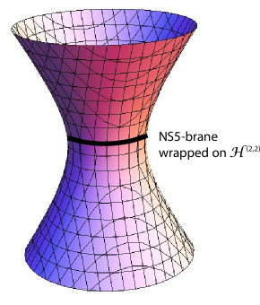
Figure 2: NS5-brane source wrapped on the $\psi\in[0,4\pi)$ cycle of ${\cal H}^{(2,2)}$ and smeared in the transverse $S^{2}$ directions of the bulk solution (4.19).

With the inclusion of this source, the relevant part of the Einstein equation for the static Salam-Sezgin + NS5 background, with 4D gravity fluctuations, is, after multiplication on both sides by $H^{2}$,

$${1\over 16\pi G_{{\scriptscriptstyle 10}}}\left(g^{2}\eta_{\mu\nu}\triangle_{\rm{\scriptscriptstyle EH}}\tilde{H}-H^{2}\square_{(4)}h_{\mu\nu}\xi-g^{2}Hh_{\mu\nu}\triangle_{\rm{\scriptscriptstyle EH}}\xi\right)=-T{g^{4}\over\sqrt{g_{\rm{\scriptscriptstyle EH}}}}(\eta_{\mu\nu}-h_{\mu\nu}\,\xi(\rho))\delta^{2}(z)\,,$$ (5.2)

where $H$ and $\tilde{H}$ are as in (4.15) and (4.16), and $G_{{\scriptscriptstyle 10}}$ is the 10D Newton constant. Owing to the smearing of the source in the $S^{2}$ directions, the relevant transverse space is reduced to just two dimensions; hence one has just the two-dimensional $\delta^{2}(z)$ delta function, for $z^{a}=(r,\chi)$, on the right-hand side of (5.2).

For the static background with $\tilde{H}=-k\log\tanh\rho\sim-k\log\rho$, Equation (5.2) gives

$$\int\sqrt{g_{\rm{\scriptscriptstyle EH}}}\triangle_{\rm{\scriptscriptstyle EH}}\tilde{H}=-16\pi G_{{\scriptscriptstyle 10}}Tg^{2}\,.$$ (5.3)

Performing the integral while noting that $\sqrt{g_{\rm{\scriptscriptstyle EH}}}=\frac{1}{8}\cosh 2\rho\sinh 2\rho\sin\theta\rightarrow\frac{1}{4}\rho\sin\theta$ as $\rho\to 0$, and that

$$d^{2}z\delta^{2}(z)={1\over 2\pi}d\rho d\chi\delta(\rho)$$ (5.4)

for $\mbox{SO}(2)$ invariant (i.e. $\chi$-independent) functions, and using the explicit form of $\tilde{H}$, one obtains on the left-hand side $\frac{\pi}{2}\rho{\partial\over\partial\rho}\tilde{H}$. One thus gets the following relation between $k$ and $T$:

$$k=32G_{{\scriptscriptstyle 10}}Tg^{2}\,.$$ (5.5)

5.1 Fluctuations about the NS5-brane

Having identified the relation (5.5) between the 10D bulk solution integration constant $k$ and the NS5-brane source tension $T$, one can confront the analysis of gravitational $h_{\mu\nu}(x,\rho)$ fluctuations around the static $\hbox{Salam-Sezgin}+\hbox{NS5}$ background. From the different factors of $H$ in the sourced equation (5.2), one finds that the sourced eigenvalue problem relevant to 4D gravitational fluctuations with $\hbox{mass}^{2}=g^{2}\lambda$ is

$${1\over 16\pi G_{{\scriptscriptstyle 10}}}\left(\triangle_{\rm{\scriptscriptstyle EH}}\xi_{\lambda}(\rho)+\lambda H\xi(\rho)\right)=-T{g^{2}\over H\sqrt{g_{\rm{\scriptscriptstyle EH}}}}\xi_{\lambda}(\rho)\delta^{2}(z)\,.$$ (5.6)

At this point, one hopes to use the sourced equation (5.6) to determine the relevant boundary conditions as $\rho\to 0$ for the transverse wavefunction $\xi_{\lambda}(\rho)$. A standard Frobenius analysis of the eigenfunction problem shows that as $\rho\to 0$, $\xi_{\lambda}(\rho)$ has the following asymptotic behaviour, both in the original Salam-Sezgin background and also with the NS5-brane inclusion, and for arbitrary eigenvalue $\lambda$:

$$\xi_{\lambda}(\rho)\rightarrow a_{\lambda}+b_{\lambda}\log\rho\,.$$ (5.7)

For a transverse bound state, one requires normalizability of the transverse wavefunction $\xi_{\lambda}(\rho)$ with respect to the full norm, including also the effects of the NS5-brane inclusion via the total $H$ function (4.15),

$$||\xi||^{2}=\frac{1}{\pi^{2}}\int d^{4}z_{\rm{\scriptscriptstyle EH}}H\sqrt{g_{\rm{\scriptscriptstyle EH}}}|\xi|^{2}\,.$$ (5.8)

Overall normalizability, including all contributions from $\rho\in(0,\infty)$, will determine an overall normalisation constant for $\xi_{\lambda}$. But we also need to know the asymptotic value for the ratio $a_{\lambda}/b_{\lambda}$, which can be parametrised by $\varpi=\arctan({a_{\lambda}\over b_{\lambda}})$. Numerical study of the eigenvalue problem shows that there is a one-to-one relationship $\varpi(\lambda)$ between the eigenvalue $\lambda$ and $\varpi$, with $\varpi=0$ corresponding to $\lambda=0$.

Unlike the situation as $\rho\to\infty$, where the requirement of normalizability selects the most strongly falling $\xi_{\lambda}(\rho)$ solution with $\lambda<1+k$ for candidate bound state wavefunctions, as we saw for $\Psi_{\lambda}$ in (3.14), normalizability considerations with respect to the norm (5.8) as $\rho\to 0$ do not fix the value of $\varpi$ for the asymptotic limit of the transverse $\xi(\rho)$ wavefunction. This is due to the $\sinh 2\rho$ factor in $\sqrt{g_{\rm{\scriptscriptstyle EH}}}$ for the Eguchi-Hanson metric (2.16), which allows any value of $\varpi$ to correspond to a normalizable wavefunction. The boundary condition for $\varpi$ has to come instead from a careful consideration of the effects of the delta-function source term in (5.6).

Even taking into account the sourced equation (5.6), determining the asymptotic value of $\varpi$ is somewhat elusive. The obvious thing to try to do is to multiply (5.6) by $\sqrt{g_{\rm{\scriptscriptstyle EH}}}$ and then to integrate over a small volume surrounding $\rho=0$ (this volume corresponds to a $D_{2}$ disk in $(\rho,\chi)$ times an $S^{2}$ sphere for the angular directions $(\theta,\varphi)$). However, noting that $H$ has the asymptotic behaviour (4.21) as $\rho\to 0$, one finds that the $b_{\lambda}\log\rho$ asymptotic part of (5.7) simply reproduces the $k$ to $T$ relation (5.5) while the $a_{\lambda}$ part of (5.7) is eliminated in the $\rho\to 0$ limit after division by $H$ on the right-hand side, and similarly drops out of the left-hand side of the integral of (5.6).

In order to determine the asymptotic value of $\varpi$ for the transverse wavefunction, one needs to be more careful and employ a regularised approach to the $\delta^{2}(\rho,\chi)$ delta function in the sourced equation (5.6). The support domain of the delta-function source needs to be expanded out slightly, to become a ring at radius $\rho=\epsilon$. Subsequently, we will take a limit in which $\epsilon$ is shrunk to zero. Thus, one replaces the pointlike delta-function at the center of the $D_{2}$ integration disk by a ring delta-function

$$d^{2}z\delta^{2}(z)=\frac{1}{2\pi}d\rho d\chi\delta(\rho-\epsilon)\,.$$ (5.9)

Integrating the NS5-sourced equation (5.6) over a small volume including the delta-function source extending from $\epsilon_{-}<\epsilon$ to $\epsilon_{+}>\epsilon$, one gets

$$\int_{\epsilon_{-}}^{\epsilon_{+}}\sqrt{g_{\rm{\scriptscriptstyle EH}}}\,\triangle_{\rm{\scriptscriptstyle EH}}\xi_{\lambda}=-16\pi G_{{\scriptscriptstyle 10}}Tg^{2}\int_{\epsilon_{-}}^{\epsilon_{+}}d\rho{\xi_{\lambda}\over H}\delta(\rho-\epsilon)\,.$$ (5.10)

Performing the integral and recalling that $H\to-k\log\rho$ as $\rho\to 0$, one gets

$$\frac{\pi}{2}\rho{\partial\over\partial\rho}\xi_{\lambda}\Big{|}_{\epsilon_{-}}^{\epsilon_{+}}={16\pi G_{{\scriptscriptstyle 10}}Tg^{2}\over k}\int_{\epsilon_{-}}^{\epsilon_{+}}{\xi_{\lambda}\over\log\rho}\delta(\rho-\epsilon)d\rho\,.$$ (5.11)

Note that inside the ring delta-function source, the wavefunction solution $\xi_{\lambda}$ must be singularity-free, and thus must be entirely composed of the constant asymptotic solution

$$\xi_{\lambda}(\rho)|_{\hbox{\small in}}=a_{\lambda}\,,$$ (5.12)

so that inside the source one has ${\partial\xi_{\lambda}\over\partial\rho}|_{\hbox{\small in}}=0$. Letting the asymptotic value of the $\xi_{\lambda}(\rho)$ wavefunction outside the source be

$$\xi_{\lambda}(\rho)|_{\hbox{\small out}}=\tilde{a}_{\lambda}+b_{\lambda}\log\rho\,,$$ (5.13)

one accordingly has the continuity relation for the undifferentiated wavefunction

$$\xi_{\lambda}(\rho)|_{\hbox{\small in}}=a_{\lambda}=\tilde{a}_{\lambda}+b_{\lambda}\log\epsilon=\xi_{\lambda}(\rho)|_{\hbox{\small out}}\,,$$ (5.14)

while from (5.11) one obtains the discontinuity in ${\partial\xi_{\lambda}\over\partial\rho}$:

$$\rho{\partial\xi_{\lambda}\over\partial\rho}\Big{|}_{\epsilon_{-}}^{\epsilon_{+}}=b_{\lambda}={32G_{{\scriptscriptstyle 10}}Tg^{2}\over k}{(\tilde{a}_{\lambda}+b_{\lambda}\log\epsilon)\over\log\epsilon}\,,$$ (5.15)

which implies

$$b_{\lambda}\left(1-{32G_{{\scriptscriptstyle 10}}Tg^{2}\over k}\right)={32G_{{\scriptscriptstyle 10}}Tg^{2}\over k}{\tilde{a}_{\lambda}\over\log\epsilon}\,.$$ (5.16)

Hence the regularised relation between the $\rho\to 0$ asymptotic coefficients in the solution outside the source is

$$\tilde{a}_{\lambda}=b_{\lambda}({k\over 32G_{{\scriptscriptstyle 10}}Tg^{2}}-1)\log\epsilon\,.$$ (5.17)

At the same time, the relation (5.5) between $k$ and $T$ is now also modified. Instead of relation (5.3), one now has

$$\int_{\epsilon_{-}}^{\epsilon_{+}}d\rho\sqrt{g_{\rm{\scriptscriptstyle EH}}}\,\triangle_{\rm{\scriptscriptstyle EH}}\tilde{H}=-16\pi G_{{\scriptscriptstyle 10}}Tg^{2}\int_{\epsilon_{-}}^{\epsilon_{+}}d\rho\delta(\rho-\epsilon)=-16\pi G_{{\scriptscriptstyle 10}}Tg^{2}\,.$$ (5.18)

Recalling that inside the source the solution has to be singularity-free, so $\tilde{H}_{\hbox{\small in}}=0$, i.e. inside the source there is no NS-5 brane back-reaction, while outside the source one has the fully back-reacted solution with $H=\tilde{H}+H_{SS}$, one can perform the integral on the left-hand side to obtain

$$\frac{\pi}{2}\rho{\partial\over\partial\rho}(-k\log\tanh\rho)\Big{|}_{\epsilon_{-}}^{\epsilon_{+}}=-16\pi G_{{\scriptscriptstyle 10}}Tg^{2}\,.$$ (5.19)

Now

$$\rho{\partial\over\partial\rho}(-k\log\tanh\rho)={\rho\over\tanh\rho}\left(1-\tanh^{2}\rho\right)\rightarrow 1-\frac{2}{3}\rho^{2}$$ (5.20)

as $\rho\to 0$, so the regularised $k\leftrightarrow T$ relation becomes

$$-k(1-\frac{2}{3}\rho^{2})=-32G_{{\scriptscriptstyle 10}}Tg^{2}\,,$$ (5.21)

which implies

$${k\over 32G_{{\scriptscriptstyle 10}}Tg^{2}}-1=\frac{2}{3}\epsilon^{2}+{\cal O}(\epsilon^{4})\,.$$ (5.22)

If one takes the limit $\epsilon\to 0$ at this point in (5.22), one simply reobtains (5.5). However, a careful derivation of the boundary condition for $\varpi$ from the sourced fluctuation problem (5.6, 5.9) requires combining the regularised $k\leftrightarrow T$ relation with the regularised exterior $a_{\lambda}\leftrightarrow b_{\lambda}$ relation (5.17). Putting these two equations together, one obtains

$$a_{\lambda}=\frac{2}{3}b_{\lambda}\epsilon^{2}\log\epsilon+{\cal O}(\epsilon^{4})\,,$$ (5.23)

and so, upon finally taking the limit $\epsilon\to 0$, one finds the requirement

$$a_{\lambda}/b_{\lambda}\rightarrow 0\ \ \mbox{{\it i.e.\ }}\ \varpi(\lambda)=0\,,$$ (5.24)

which for bound states corresponds uniquely to the eigenvalue $\lambda=0$.

Hence the unique bound-state wavefunction for 4D gravitational fluctuations in the presence of the NS5-brane is the zero-mode

$$\xi_{0}(\rho)=\log(\tanh\rho)\,,$$ (5.25)

which, agreeably, is exactly the same as that found in (3.17) in our preliminary Salam-Sezgin background analysis, prior to the inclusion of the NS5-brane. This is a key result of this paper: recalling that $m^{2}=g^{2}\lambda$, we have found that a careful treatment of the NS5-brane source for the transverse part of the gravitational fluctuation wavefunction shows that linearised 4D fluctuations consistent with the conditions imposed by the NS5-brane source are massless in the 4D subspace.

5.2 Asymptotic conformal invariance and self-adjointness

The delicacy needed in analysing the $\rho\to 0$ boundary condition (5.24) reflects the specific asymptotic character of the radial Schrödinger problem (3.10, 3.11), both in the original undeformed Salam-Sezgin background and also after inclusion of the NS5-brane. Taking the $\rho\to 0$ limit of the potential (3.11), one obtains

$$V_{{\scriptscriptstyle\rho}\to 0}=-{1\over 4\rho^{2}}\,.$$ (5.26)

The corresponding one-dimensional quantum mechanical problem has a long history [16, 17, 18]. A good overview is given in [19]. The special character of this one-dimensional problem involves not only the $1/\rho^{2}$ form of the potential, which gives rise to an ${\rm O}(2,1)$ 1D conformal invariance, but also the $-\frac{1}{4}$ coefficient, which is a critical value. For a potential $V=\gamma/\rho^{2}$ with coefficient $\gamma>-\frac{1}{4}$, a regularised treatment shows that there is no $L^{2}$ normalizable bound state, while for $\gamma<-\frac{1}{4}$, an infinity of discrete $L^{2}$ normalizable bound states appears. At the critical value $\gamma=-\frac{1}{4}$, there is just a single bound state.

The character of the $V=-1/(4\rho^{2})$ Schrödinger problem is exactly as we have found above in Section 5.1: the requirement of normalisation does not fix the asymptotic form of a bound-state wavefunction at the origin. A candidate bound-state wavefunction for a general value of $\lambda$ would spontaneously break the asymptotic 1D conformal invariance. The one exception to this is the $\lambda=0$ wavefunction that we found in (5.24).

Another key feature of the $V=-1/(4\rho^{2})$ Schrödinger problem is the delicate issue of self-adjointness of the corresponding Hamiltonian, or, in our case, of the $-{d^{2}\over d\rho^{2}}$ part of the wave operator (3.10). For two normalizable candidate bound-state wavefunctions $\Psi_{1}$ and $\Psi_{2}$, self-adjointness of this operator requires $\int_{0}^{\infty}(\Psi_{1}^{\ast}{d^{2}\over d\rho^{2}}\Psi_{2}-\Psi_{2}{d^{2}\over d\rho^{2}}\Psi_{1}^{\ast})=0$, which in turn requires

$$(\Psi_{1}^{\ast}{d\over d\rho}\Psi_{2}-\Psi_{2}{d\over d\rho}\Psi_{1}^{\ast}){\Big{|}}_{0}^{\infty}=0\,.$$ (5.27)

For normalizable bound-state wavefunctions, there is no problem with this requirement as $\rho\to\infty$, but for $\Psi_{1}$ and $\Psi_{2}$ having $\rho\to 0$ asymptotic structure $\sqrt{\rho}(a_{i}+b_{i}\log\rho)$ (corresponding to (5.7) for rescaled wavefunctions (3.9), with $i=1,2$) the condition (5.27) requires

$$\frac{a_{1}}{b_{2}}=\frac{a_{2}}{b_{2}}\,,$$ (5.28)

i.e. $\Psi_{1}$ and $\Psi_{2}$ must have the same eigenvalue $\lambda$, since $a_{\lambda}/b_{\lambda}$ is a single-valued function of $\lambda$, as we have seen.

This is the underlying reason for the existence of precisely one bound-state eigenfunction. In our case, coupling to the NS5-brane source as in (5.6) selects $\lambda=0$. In the case of the classic $V=-1/(4\rho^{2})$ Schrödinger problem, this would not be very good, because it would put the single allowed bound state right at the edge of the continuum of scattering states. However, in the present case, the potential (3.11) deviates from the $-1/(4\rho^{2})$ structure as $\rho$ increases away from zero. This has the effect of raising the edge of the continuous spectrum up to $\lambda=1+k$, as we have seen above in Sections 3.1 and 5.1.

6 The braneworld Newton constant

Having established that there exists a zero-eigenvalue bound-state transverse wave function (3.17), the basic aim of constructing a type IIA supergravity brane configuration that localises massless gravity in a four-dimensional brane subspace has been achieved. A key achievement of this construction is the non-zero value of Newton’s constant for the massless effective gravity theory in the 4D subspace, despite the infinite volume of the transverse space. Starting from the Einstein-frame gravitational action for the 10D metric $\hat{g}_{MN}$

$$I_{{\scriptscriptstyle 10}}={1\over 16\pi G_{{\scriptscriptstyle 10}}}\int d^{10}x\sqrt{\hat{g}}\hat{R}(\hat{g})\,,$$ (6.1)

the effective theory for 4D gravitational fluctuations is obtained starting from the Einstein-frame form $ds_{10\,\rm ein}^{2}=e^{-\phi/2}ds_{10\,\rm str}^{2}$ of the static string-frame metric given in (4.19) and making the replacement $\eta_{\mu\nu}\rightarrow\eta_{\mu\nu}+h_{\mu\nu}(x)\xi(\rho)$, as we have done above in Sections 3 and 5. The angular coordinates $\psi,\theta,\phi$ and $\chi$, for which we are considering only S-waves without further excitation, give rise to compact integrals producing corresponding factors of $g$ (with length dimension $-1$) in the effective theory. In order to obtain a 4D effective theory, we compactly also the $y$ coordinate with a circumference $\ell_{y}$. Recalling that $\psi$ takes values in the range $[0,4\pi)$, one finds at quadratic order in $h_{\mu\nu}(x)$ an effective action for 4D linearised gravity

$$I_{\rm{\scriptscriptstyle lin\,4}}={1\over\upsilon_{0}^{2}}\int d^{4}x\left(-\frac{1}{2}\partial_{\sigma}h_{\mu\nu}\partial^{\sigma}h^{\mu\nu}+\frac{1}{2}\partial_{\mu}h^{\sigma}{}_{\sigma}\partial^{\mu}h^{\tau}{}_{\tau}+\partial^{\nu}h_{\mu\nu}\partial^{\sigma}h^{\mu}{}_{\sigma}+h^{\sigma}{}_{\sigma}\partial^{\mu}\partial^{\nu}h_{\mu\nu}\right)\,,$$ (6.2)

where

$$\upsilon_{0}=\left({16\pi G_{{\scriptscriptstyle 10}}g^{5}\over\pi^{2}\ell_{y}I_{2}}\right)^{\frac{1}{2}}\,,$$ (6.3)

in which

$$I_{2}=\int_{0}^{\infty}d\rho H\sinh 2\rho\cosh 2\rho\,\xi_{0}^{2}=\frac{\pi^{2}}{24}(2+3k)\,.$$ (6.4)

Note that, up to a factor ${2\pi^{3}\over g^{5}}$, $I_{{\scriptscriptstyle 2}}$ is just the $(\hbox{norm})^{2}$ (5.8) of $\xi_{0}$. Combining Eqns (6.3) and(6.4), one has the normalisation factor

$$\upsilon_{0}=\left({384G_{{\scriptscriptstyle 10}}g^{5}\over\pi^{3}\ell_{y}(2+3k)}\right)^{\frac{1}{2}}\,.$$ (6.5)

If it were not for the normalizable character of the zero-mode $\xi_{0}(\rho)$, one would obtain a vanishing value for $\upsilon_{0}$. This is what would happen for a standard Kaluza-Klein reduction to the $\rho$-independent sector of the theory, as in [13], where $\xi_{0}(\rho)$ is simply a constant. In order to calculate the effective 4D Newton’s constant, one now needs to rescale $h_{\mu\nu}=\upsilon_{0}\tilde{h}_{\mu\nu}$ in order to obtain a canonically-normalised kinetic term (6.2) for $\tilde{h}_{\mu\nu}$. Then the leading effective 4D coupling $\kappa_{4}=\sqrt{32\pi G_{{\scriptscriptstyle 4}}}$ for gravitational self-interactions is obtained from the coefficient in the trilinear terms in $\tilde{h}_{\mu\nu}$ in the 4D effective action. These involve an integral

$$I_{3}=\int_{0}^{\infty}d\rho H\sinh 2\rho\cosh 2\rho\,\xi_{0}^{3}=-{3(1+2k)\,\zeta(3)\over 4}\,.$$ (6.6)

The $\sinh 2\rho$ factor in (6.6), arising from $\sqrt{g_{\rm{\scriptscriptstyle EH}}}$, leads to the convergence of (6.6) in the limit as $\rho\to 0$, just as it does for $I_{2}$. The 4D massless gravitational coupling $\kappa_{4}^{(0)}=\sqrt{32\pi G_{{\scriptscriptstyle 4}}}$ is then obtained upon rescaling $h_{\mu\nu}=\upsilon_{0}\tilde{h}_{\mu\nu}$ so as to obtain a conventionally normalised quadratic action for $\tilde{h}_{\mu\nu}$, and then extracting the coefficient of the trilinear $\tilde{h}_{\mu\nu}$ terms in the effective action:

$$\kappa_{4}^{(0)}=\left|\left({16\pi G_{{\scriptscriptstyle 10}}g^{5}\over\pi^{2}\ell_{y}}\right)^{\frac{1}{2}}{I_{3}\over(I_{2})^{\frac{3}{2}}}\right|\,.$$ (6.7)

Using (6.4) and (6.6), this becomes

$$\kappa_{4}^{(0)}=144\sqrt{6}\zeta(3)\left({G_{{\scriptscriptstyle 10}}g^{5}\over\pi^{7}\ell_{y}}\right)^{\frac{1}{2}}{(1+2k)\over(2+3k)^{\frac{3}{2}}}\,,$$ (6.8)

and so the 4D Newton constant is given by

$$G_{{\scriptscriptstyle 4}}={3888\,\zeta(3)^{2}G_{{\scriptscriptstyle 10}}g^{5}\over\pi^{8}\ell_{y}}{(1+2k)^{2}\over(2+3k)^{3}}\,.$$ (6.9)

Evaluating gravitational couplings to matter, as opposed to the gravitational self-coupling, requires setting up a model of non-gravitational matter in the 4D subspace. One approach to this would be to employ a Hořava-Witten construction [20], replacing the $S^{1}$ compactification of the $y$ direction by a $S^{1}/{{\mathbb{Z}}}_{2}$ orbifold. One way to view this would be as a 7D to 6D reduction starting from the 7D theory on ${\cal H}^{(2,2)}$ [13], thus obtaining a 6D chiral $(1,0)$ supersymmetric theory with potential anomalies arising from anomaly inflow, and hence requiring compensating 6D matter fields [22]. Another way to view it would be as a 5D to 4D reduction after the additional $S^{2}\ \&\ \hbox{monopole}$ reduction from 7D, thus producing a 4D chiral N=1 supersymmetric theory, again with anomaly inflow requiring compensating 4D matter fields [21]. Either of these two $S^{1}/{{\mathbb{Z}}}_{2}$ approaches would have the additional effect of reducing the final surviving supersymmetry to $N=1$ in 4D, which could be of practical physical interest. A simpler approach to modelling matter fields, however, which is all that we shall consider here, is just to consider the non-gravitational 4D fields accompanying gravity in the descent to 4D from 10D type IIA supergravity. From the string-frame unbroken supersymmetry (4.25), one sees that superpartners of the graviton should involve the same $\xi_{0}$ transverse wavefunction, giving rise to bilinear kinetic and trilinear gravitational effective-action terms involving the same $I_{2}$ and $I_{3}$ integrals as for the gravitational self-coupling, and hence the same $\kappa_{4}$ gravitational coupling constant (6.8).

7 Corrections to 4D Newtonian gravity

Finally, let us sketch the consequences of the continuum of $\lambda\neq 0$ transverse gravitational eigenmodes. The corresponding 4D $h_{\mu\nu}^{(\lambda)}$ massive gravitational modes are separated from the massless 4D gravitational states with transverse eigenmode $\xi_{0}$ by a gap in $(\hbox{mass})^{2}$ eigenvalues of height $(1+k)g^{2}$, as we have seen. For $\lambda>1+k$, as seen in Section 3.1 (but now with the NS5-brane moving the edge of the continuum from $\lambda=1$ to $\lambda=1+k$), the transverse $\xi_{\lambda}(\rho)$ eigenfunctions have oscillatory behaviour as $\rho\to\infty$, instead of the rising or falling exponential behaviour of the candidate bound states for $\lambda<1+k$. The boundary-condition implications of the NS5-brane source as analysed in Section 5.1 remain valid also for $\lambda\neq 0$ eigenmodes: a general Frobenius analysis shows that their $\rho\to 0$ asymptotics have to be as in (5.7), but the constraints of the NS5-brane source imply that the asymptotic constant part of a $\xi_{\lambda\neq 0}$ wavefunction must vanish, just as it must for $\xi_{0}$. For the candidate $\lambda<1+k$ bound states, it is only for $\lambda=0$ that this boundary condition proves to be consistent with the other boundary condition needing to be imposed as $\rho\to\infty$: elimination of the most weakly falling exponential term, in order to obtain normalizability. However, for the continuum of $\lambda>1+k$ wave functions, one does not demand standard normalizability with respect to the norm (5.8). Instead, just as in free-field theory, continuum wavefunctions need to be delta-function orthonormalised.

Gravitational fluctuations involving $\lambda\neq 0$ transverse $\xi_{\lambda}$ eigenmodes make small contributions to the 4D effective action. Starting from the edge of the continuous transverse spectrum at $\lambda=1+k$, one sees from (3.8) that the spectrum of gravitational modes arising from the transverse dynamics will have continuous $(\hbox{mass})^{2}$ eigenvalues ranging over the interval $(1+k)g^{2}\leq m^{2}\leq\infty$. Repeating the normalisation analysis for such $\xi_{\lambda}$ modes, one finds that in order to have canonically normalised kinetic terms, the $h_{\mu\nu}^{(\lambda)}$ massive graviton fields require rescaling by

$$\upsilon_{\lambda}=\left({16\pi G_{{\scriptscriptstyle 10}}g^{5}\over\pi^{2}\ell_{y}}\right)^{\frac{1}{2}}{\cal N}_{\lambda}\,,$$ (7.1)

where ${\cal N}_{\lambda}$ is a normalisation coefficient depending on the details of $\xi_{\lambda}$.

Assuming that matter interacting with the continuum of massive gravitational modes itself has transverse wavefunction $\xi_{0}$, its interaction with such massive gravitational modes at the trilinear level involves an integral

$$I_{2,\lambda}=\int_{0}^{\infty}d\rho H\sinh 2\rho\cosh 2\rho\,\xi_{0}^{2}\,\xi_{\lambda}\,,$$ (7.2)

which is convergent as $\rho\to 0$ owing to the $\sinh 2\rho$ term, and as $\rho\to\infty$ owing to the $e^{-2\rho}$ asymptotic falloff of $\xi_{0}$. Rescaling all fields in order to produce canonical kinetic terms then gives rise to the coupling between $h_{\mu\nu}^{(\lambda)}$ and 4D matter:

$$\kappa_{4}^{(\lambda)}=\left|\left({16\pi G_{{\scriptscriptstyle 10}}g^{5}\over\pi^{2}\ell_{y}}\right)^{\frac{1}{2}}{I_{2,\lambda}\over I_{2}}{\cal N}_{\lambda}\right|={24\over\pi^{2}(2+3k)}\left|\left({16\pi G_{{\scriptscriptstyle 10}}g^{5}\over\pi^{2}\ell_{y}}\right)^{\frac{1}{2}}I_{2,\lambda}\,{\cal N}_{\lambda}\right|\,.$$ (7.3)

Any given continuum massive gravitational mode will produce a Yukawa correction

$$\Delta V_{\lambda}=-(\kappa_{4}^{(\lambda)})^{2}M_{1}M_{2}{e^{-g\sqrt{\lambda}|x|}\over|x|}$$ (7.4)

to the 4D Newtonian $V=-(\kappa_{4}^{(0)})^{2}M_{1}M_{2}/|x|$ potential, where $|x|$ is the distance between masses $M_{1}$ and $M_{2}$ in the 4D subspace. If one assumes that $\kappa_{4}^{(\lambda)}$ does not have a strong dependence on $\lambda$ for $\lambda\gtrapprox 1+k$, and noting that for large $\lambda$ the falling exponential suppresses $\Delta V_{\lambda}$ contributions, then one obtains an integrated correction to the Newtonian potential

$$\Delta V = \int_{1+k}d\lambda\Delta V_{\lambda}$$ (7.5)

$$\simeq -{2M_{1}M_{2}(\kappa_{4}^{(1+k)})^{2}e^{-g\sqrt{(1+k)}|x|}\over g|x|^{2}}\left((1+k)^{\frac{1}{2}}+{1\over g|x|}\right)\,.$$

Note that the corrections to the Newtonian potential have leading behaviour ${e^{(-g\sqrt{(1+k)}|x|)}\over g|x|^{2}}$ here instead of the ${1\over|x|^{3}}$ leading correction in [2], because the edge of the continuous spectrum in the present construction is located at $m^{2}=g^{2}(1+k)$ instead of $m^{2}=0$.

8 Conclusion

The hyperbolic background with NS5-brane construction that we have given in this paper provides a successful localisation of gravity in a lower-dimensional subspace of type IIA supergravity. In doing so, it has evaded a number of problems with braneworld gravity localisation that have been raised in the literature. A fuller analysis will be needed to understand how this construction may be generalised to other situations, but we may identify a number of features of our construction that help to evade some of the problems that have been raised. In the discussions that arose following Ref. [2], which was based on the junction of AdS slices, a “no-go” theorem was put forward in Ref. [29]. This ruled out braneworld reductions that are non-singular or with singularities satisfying an admissibility criterion that the $g_{00}$ component of the metric should not increase as one approaches the singularity (which our NS5-brane construction satisfies). However, that analysis assumed that the scalar-field potential is non-positive. This is clearly not the case for the ${\rm SO}(2,2)$ invariant potential of the 7D theory [13] obtained via ${\cal H}^{(2,2)}$ reduction, which is positive-definite, generalising the positive potential of the Salam-Sezgin model [12]. The positivity of this potential is key to allowing a solution incorporating an $S^{2}$ and 4D flat space – otherwise, reduction on an $S^{2}$ factor would give rise to an anti-de Sitter space in 4D. The noncompact ${\rm SO}(2,2)$ invariant structure is a consequence of the underlying hyperbolic geometry, which thus appears to be a key feature of our successful construction.

A more substantial potential problem with braneworld localisations related to our construction was outlined in Ref. [7]. Indeed, a simple argument was given there that would seem to imply that a localisation producing massless effective gravity in the lower dimension of a spacetime with infinite transverse geometry can only be made with a constant transverse wavefunction. This would seem to rule out normalisable bound states yielding massless gravity. However, a key feature of that argument involves integration by parts of one of the derivatives in the transverse wave operator. In the corresponding integration by parts in our construction, one cannot ignore the surface term, and so the demonstration that the wavefunction $\xi_{0}$ has to be constant fails in our case. This does, however raise the issue of self-adjointness of the transverse wave operator, which we have discussed in Section 5.2. Provided there is just one bound state, the wave operator can be self-adjoint, as in our case with the single transverse bound state $\xi_{0}$. So another important feature of our construction appears to be this quite special behaviour of the transverse eigenvalue problem near the $\rho=0$ “waist” of the ${\cal H}^{(2,2)}$ space, which also can be viewed as the apex of the underlying Eguchi-Hanson space.

The present construction has been purely classical, focusing only on a supergravity realisation. Since the only elements used, i.e. type IIA supergravity and an NS5-brane, are also native objects in string theory, the construction carries over directly into string theory. From that point of view, the solution for $e^{\phi}$ in the fully NS5 back-reacted solution (4.19) with $H$ given by (4.17), i.e. with an asymptotic $e^{-2\rho}$ behaviour, shows that the solution has asymptotically $\phi\propto-\rho$: it asymptotically tends to a linear-dilaton string-theory vacuum. The eight-supercharge unbroken supersymmetry (2.19, 2.20) of the back-reacted solution guarantees stability. This remains so should one decide to sacrifice half of this supersymmetry either by reducing the $y$ coordinate on $S^{1}/{{\mathbb{Z}}}_{2}$, or by making a corresponding Hořava-Witten construction, leaving just $N=1$ supersymmetry in four dimensions. At the quantum level, some usual additional considerations will come into play. For example, the NS5-brane charge $T$ will have to take its value on a quantised charge lattice, following from Dirac-Schwinger-Zwanziger quantisation conditions [30, 31, 32].

Duality symmetries will yield other realisations of the construction given in this paper. For example, a T-duality transformation will change the present 10D type IIA solution into a solution of type IIB supergravity. Depending on whether this is done in a worldvolume or in a transverse direction (e.g. in one of the smeared transverse angle coordinates), one can get a 4-brane or an ALF space [33]. A general understanding of the duality maps of the present construction may help to categorise situations in which localised braneworld gravity can exist.

The gravity-localising construction given in this paper is not a dimensional reduction: at all stages, we have been working with solutions of 10D supergravity. Although reduction on ${\cal H}^{(2,2)}$ produces a consistent Kaluza-Klein truncation [13] to the ${\rm SO}(2,2)$ invariant theory containing the Salam-Sezgin model, in the present paper we have not sought to eliminate dependence on all the transverse coordinates. For simplicity, we have considered “S-wave” solutions independent of the transverse-coordinate angles $\theta,\,\phi$ and $\chi$, but this restriction could straightforwardly be relaxed. Our construction depends in a fundamental way, however, on the transverse radial coordinate $\rho$, and the effective theory derived from the transverse zero-mode $\xi_{0}(\rho)$ is not a consistent Kaluza-Klein truncation. The continuum of massive modes lying above the $g\,\sqrt{1+k}$ mass gap produce small corrections to the leading-order massless braneworld gravity. In Section 7, we have made a preliminary sketch of these corrections, but this question clearly deserves a more complete study.

References

- [1] V. A. Rubakov and M. E. Shaposhnikov, “Do we live inside a domain wall?,” Phys. Lett. B 125 (1983) 136.
- [2] L. Randall and R. Sundrum, “An alternative to compactification,” Phys. Rev. Lett. 83 (1999) 4690, hep-th/9906064.
- [3] A. Karch and L. Randall, “Locally localized gravity,” JHEP 0105 (2001) 008, hep-th/0011156.
- [4] A. Brandhuber and K. Sfetsos, “Nonstandard compactifications with mass gaps and Newton’s law,” JHEP 9910 (1999) 013, hep-th/9908116.
- [5] M. J. Duff, J. T. Liu and K. S. Stelle, “A supersymmetric type IIB Randall-Sundrum realization,” J. Math. Phys. 42 (2001) 3027, hep-th/0007120.
- [6] J. L. Lehners, P. Smyth and K. S. Stelle, “Kaluza-Klein induced supersymmetry breaking for braneworlds in type IIB supergravity,” Nucl. Phys. B 790 (2008) 89, arXiv:0704.3343 [hep-th].
- [7] C. Bachas and J. Estes, “Spin-2 spectrum of defect theories,” JHEP 1106 (2011) 005, arXiv:1103.2800 [hep-th].
- [8] C. M. Hull and N. P. Warner, “Noncompact gaugings from higher dimensions,” Class. Quant. Grav. 5 (1988) 1517.
- [9] B. de Wit, H. Samtleben and M. Trigiante, “Magnetic charges in local field theory,” JHEP 0509 (2005) 016, hep-th/0507289.
- [10] R. Gueven, “Black p-brane solutions of D = 11 supergravity theory,” Phys. Lett. B 276 (1992) 49.
- [11] H. Lü, C. N. Pope and K. S. Stelle, “Vertical versus diagonal dimensional reduction for p-branes,” Nucl. Phys. B 481 (1996) 313, hep-th/9605082.
- [12] A. Salam and E. Sezgin, “Chiral compactification on Minkowski of Einstein-Maxwell supergravity in six dimensions,” Phys. Lett. B147 (1984) 47.
- [13] M. Cvetič, G. W. Gibbons, and C. N. Pope, “A string and M-theory origin for the Salam-Sezgin model,” Nucl. Phys. B 677 (2004) 164, hep-th/0308026.
- [14] C. Csaki, J. Erlich, T. J. Hollowood and Y. Shirman, “Universal aspects of gravity localized on thick branes,” Nucl. Phys. B 581 (2000) 309, hep-th/0001033.
- [15] M. Cvetič, H. Lü and C. N. Pope, “Brane resolution through transgression,” Nucl. Phys. B 600 (2001) 103, hep-th/0011023.
- [16] K. M. Case, “Singular potentials,” Phys. Rev. 80 (1950) 797.
- [17] L. Landau and E.M. Lifshitz, “Quantum Mechanics,” (Pergamon, London, 1960).
- [18] V. de Alfaro, S. Fubini and G. Furlan, “Conformal invariance in quantum mechanics,” Nuovo Cim. A 34 (1976) 569.
- [19] A. M. Essin and D. J. Griffiths “Quantum mechanics of the potential,” Am. J. Phys. 74, 109 (2006); http://dx.doi.org/10.1119/1.2165248.
- [20] P. Horava and E. Witten, “Eleven-dimensional supergravity on a manifold with boundary,” Nucl. Phys. B 475 (1996) 94, hep-th/9603142.
- [21] A. Lukas and K. S. Stelle, “Heterotic anomaly cancellation in five-dimensions,” JHEP 0001 (2000) 010, hep-th/9911156.
- [22] T. G. Pugh, E. Sezgin and K. S. Stelle, “ / heterotic supergravity with gauged R-symmetry,” JHEP 1102 (2011) 115, arXiv:1008.0726 [hep-th].
- [23] T. Eguchi and A. J. Hanson, “Selfdual solutions to Euclidean gravity,” Annals Phys. 120 (1979) 82.
- [24] V. A. Belinsky, G. W. Gibbons, D. N. Page and C. N. Pope, “Asymptotically Euclidean Bianchi IX metrics in quantum gravity,” Phys. Lett. B 76 (1978) 433.
- [25] M. J. Duff and K. S. Stelle, “Multimembrane solutions of supergravity,” Phys. Lett. B 253 (1991) 113.
- [26] K. Skenderis and M. Taylor, “Branes in AdS and pp wave space-times,” JHEP 0206 (2002) 025, hep-th/0204054.
- [27] I. A. Bandos, A. Nurmagambetov and D. P. Sorokin, “The type IIA NS5-brane,” Nucl. Phys. B 586, 315 (2000), hep-th/0003169.
- [28] H. Lü and J. F. Vazquez-Poritz, “Resolution of overlapping branes,” Phys. Lett. B 534 (2002) 155, hep-th/0202075.
- [29] J. M. Maldacena and C. Nunez, “Supergravity description of field theories on curved manifolds and a no go theorem,” Int. J. Mod. Phys. A 16 (2001) 822, hep-th/0007018.
- [30] R. I. Nepomechie, “Magnetic monopoles from antisymmetric tensor gauge fields,” Phys. Rev. D 31 (1985) 1921.
- [31] C. Teitelboim, “Gauge invariance for extended objects,” Phys. Lett. B 167 (1986) 63.
- [32] M. S. Bremer, H. Lü, C. N. Pope and K. S. Stelle, “Dirac quantization conditions and Kaluza-Klein reduction,” Nucl. Phys. B 529 (1998) 259, hep-th/9710244.
- [33] D. Tong, “NS5-branes, T duality and world sheet instantons,” JHEP 0207 (2002) 013, hep-th/0204186.