Synthesising evidence to estimate pandemic (2009) A/H1N1 influenza severity in 2009–2011

Abstract

Knowledge of the severity of an influenza outbreak is crucial for informing and monitoring appropriate public health responses, both during and after an epidemic. However, case-fatality, case-intensive care admission and case-hospitalisation risks are difficult to measure directly. Bayesian evidence synthesis methods have previously been employed to combine fragmented, under-ascertained and biased surveillance data coherently and consistently, to estimate case-severity risks in the first two waves of the 2009 A/H1N1 influenza pandemic experienced in England. We present in detail the complex probabilistic model underlying this evidence synthesis, and extend the analysis to also estimate severity in the third wave of the pandemic strain during the 2010/2011 influenza season. We adapt the model to account for changes in the surveillance data available over the three waves. We consider two approaches: (a) a two-stage approach using posterior distributions from the model for the first two waves to inform priors for the third wave model; and (b) a one-stage approach modelling all three waves simultaneously. Both approaches result in the same key conclusions: (1) that the age-distribution of the case-severity risks is “u”-shaped, with children and older adults having the highest severity; (2) that the age-distribution of the infection attack rate changes over waves, school-age children being most affected in the first two waves and the attack rate in adults over 25 increasing from the second to third waves; and (3) that when averaged over all age groups, case-severity appears to increase over the three waves. The extent to which the final conclusion is driven by the change in age-distribution of those infected over time is subject to discussion.

FLA

T1Supported in part by the Medical Research Council [Unit Programme Numbers U105260566 and U105261167], NIHR HTA Project 11/46/03, Public Health England and the Royal College of General Practitioners. , , , , , , and

1 Introduction

Evidence synthesis [e.g., Spiegelhalter, Abrams andMyles (2004), Ades and Sutton (2006)] has become an important method in epidemiology, where multiple, disparate, incomplete and often biased sources of observational (e.g., surveillance or survey) data are available to inform estimation of relevant quantities, such as prevalence and incidence of infectious disease [Welton and Ades (2005), Goubar et al. (2008), Sweeting et al. (2008), Albert et al. (2011), Presanis et al. (2011a), Birrell et al. (2011)]. Data may directly inform a quantity of interest, $\theta$, or, more usually, may indirectly inform multiple parameters $\bolds{\Theta}$ by directly informing some function of $\bolds{\Theta}$, $\psi=\psi(\bolds{\Theta})$. Such a function may represent, for example, the relationship between a biased source of data and the parameter the data should theoretically measure, so that the bias is explicitly modelled. Evidence synthesis methods combine these heterogeneous types of challenging data in a coherent manner, to estimate the “basic” parameters $\bolds{\Theta}$ and from these obtain simultaneously the “functional” parameters $\bolds{\Psi}=\{\psi_{1}(\bolds{\Theta}),\ldots,\psi_{m}(\bolds{\Theta})\}$. These functional parameters include both those directly observed and others that may not be observed but are of interest to estimate. This type of estimation typically necessitates the formulation of complex probabilistic models, often in a Bayesian framework.

Knowledge of the severity of an influenza outbreak is crucial for informing and monitoring appropriate public health responses. Severity estimates are necessary not only during a pandemic to inform immediate public health responses, but also afterwards, when a robust reconstruction of what happened during the pandemic is required to evaluate the responses. Moreover, as has happened in past influenza pandemics [Miller et al. (2009)], if a pandemic strain continues to circulate for some years, with unusual patterns of age-specific mortality, then severity estimates over time, both in terms of attack rates (the proportion of the population infected) and case-severity risks (the probability an infection leads to a severe event), are required to understand if the strain is likely to continue circulating and if severity is changing over time.

However, severity is an example epidemic characteristic that is difficult to measure directly. Typically, severity is expressed as the probability that an infection will result in a severe event, for example, death. We refer to this probability as the “case-fatality risk” ($\mathit{CFR}$). Severity may also be quantified by “case-hospitalisation” ($\mathit{CHR}$) and “case-intensive care admission” ($\mathit{CIR}$) risks, defined similarly as probabilities that an infection results in hospitalisation or intensive care (ICU) admission. Not all influenza infections will be symptomatic, where “symptomatic” may be defined in different ways, but is here taken to denote febrile influenza-like illness (ILI). Not all infections will therefore result in symptoms severe enough for a patient to access health care and hence be detectable in surveillance systems [Reed et al. (2009), Presanis et al. (2011b), Birrell et al. (2011)]. Symptomatic case-severity risks ($\mathit{sCHR},\mathit{sCIR},\mathit{sCFR}$), the probabilities a symptomatic infection leads to severe events, are therefore also considered as important indicators of severity for influenza. Estimation of these probabilities requires information on both the cumulative incidence of (symptomatic) infection over a period of time of interest (the denominator) and the cumulative incidence of severe events (the numerator). However, the denominator, whether symptomatic or all infection, is challenging to determine, due to the unobserved infections. Population-wide serological testing (testing for antibodies to influenza infection in blood serum samples) to measure the proportion of the population infected is one possibility, but is unlikely to be feasible. This challenge is only compounded in a pandemic situation, where resources and time are even more stretched than usual [e.g., Lipsitch et al. (2009), Garske et al. (2009)].

The most feasible approach to the assessment of severity is therefore via estimation, combining data from different sources and accounting for their biases, due, for example, to under-ascertainment. The majority of methods adopted to estimate influenza case-severity [e.g., Reed et al. (2009), Garske et al. (2009), Wilson and Baker (2009), Pebody et al. (2010), Wielders et al. (2012), Sypsa et al. (2011)] have not systematically accounted for all biases. Crucially, they have not made use of all available information in the estimation process, nor have they accounted for all uncertainty inherent in the data. Bayesian evidence synthesis provides a flexible framework in which all available relevant data may be coherently amalgamated, together with prior information on biases, to estimate case-severity [Lipsitch et al. (2011), McDonald et al. (2014), Presanis et al. (2009, 2011b), Shubin et al. (2013), Wu et al. (2010)].

Until the 2012/2013 winter, England experienced three waves of infection with the 2009 pandemic A/H1N1 influenza strain: in the summer of 2009, the autumn and winter of 2009–2010, and the autumn and winter of 2010–2011. The severity of the first two waves, as measured by case-severity risks, was previously estimated [Presanis et al. (2011b)] by synthesising data either from surveillance systems in place to monitor seasonal influenza or from systems set up specifically in response to the pandemic [Health Protection Agency (2010)]. In this paper, we present in detail the statistical model used in Presanis et al. (2011b) and extend the approach to estimating severity in the third wave of infection. After the first two waves, the World Health Organization declared a move to a post-pandemic period (http://www.who.int/mediacentre/news/statements/2010/h1n1_vpc_20100810/en/index.html), at which time many of thesurveillance systems that operated during the pandemic situation were either stopped or changed in form. We describe how the model of Presanis et al. (2011b) is further developed to account for these changes in the available data.

The evidence used to estimate severity in the first two waves and the changes to the surveillance systems between waves are described in Section 2. A Bayesian approach to evidence synthesis is introduced in Section 3. We then describe in Section 4 a generic model for estimating severity, before showing in Section 5.1 how the model was implemented in the first two waves. We next develop the model to estimate severity in the third wave, presenting two approaches (Sections 5.2 and 5.3, resp.). Results are given in Section 6 and we end with a discussion in Section 7.

2 Surveillance data

2.1 First & second waves

During the first two pandemic waves in 2009–2010, data were available from various surveillance systems at or used by the UK’s Health Protection Agency (HPA, now Public Health England) that provided evidence on some aspect of the pandemic, at various levels of severity. These sources indirectly informed the case-severity risks and full details of each are given in Section 1.1 of the supplementary material [Presanis et al. (2014)]. Briefly, they included the following: [(iii)]

data on laboratory-confirmed pandemic A/H1N1 cases [i.e., cases where infection with the pandemic strain was confirmed virologically, via real-time polymerase chain reaction (RT-PCR) testing of nasal or throat swabs] in the first few weeks of the pandemic [Health Protection Agency, Health Protection Scotland, Communicable Disease Surveillance CentreNorthern Ireland and National Public Health Service for Wales (2009), Health Protection Agency (2010)]. The data included dates of illness onset and information on hospital admission if it occurred, from which age group-specific case-hospitalisation risks amongst confirmed cases could be estimated. Note that these confirmed-case-hospitalisation risks are likely to be higher than the case-hospitalisation risks in all symptomatic cases, since not all symptomatic cases will have been confirmed in the first few weeks, and more severe cases in hospital are more likely to have been detected than less severe cases;

estimates of the number of symptomatic cases by week, age and region, produced by the HPA. These estimates were recognised to be under-estimates, given the data of point (iii);

serial data on age group-specific proportions of individuals with antibodies to the pandemic strain of influenza (“sero-prevalence”), from repeated cross-sectional surveys of residual sera from other (unrelated) diagnostic testing [Miller et al. (2010), Hardelid et al. (2011)]. These data indirectly inform the cumulative incidence of infection, that is, the proportion of the population infected over a period of time. Initially these data were taken at face value, but concerns about potential sampling biases led to extra sensitivity analyses (see Section 6.1);

data on laboratory-confirmed cases in hospital [Campbell et al.(2011)], including age group and dates of illness onset, hospital admission and ICU admission; and

data on the number of deaths amongst persons with confirmed pandemic A/H1N1 influenza and/or mention of influenza on the death certificate, reported to the HPA and/or the Chief Medical Officer [Donaldson et al. (2009), Pebody et al. (2010)].

2.2 Third wave

During the third wave, data sources (i), (ii) and (iv) were no longer available in the same form. Although results from testing of samples from before and after the third wave from data source (iii) are now available [Hoschler et al. (2012)], at the time of the analyses presented here, they were not accessible. Full details of each source below are given in Section 1.2 of the supplementary material [Presanis et al. (2014)].

[(vii)]

Between the second and third waves, the surveillance system for hospital admissions of confirmed cases moved to being a sentinel surveillance system, the UK Severe Influenza Surveillance Scheme (USISS). The data from this system are available at a coarser level of age aggregation and come from a sentinel sample of 23 acute NHS hospital trusts in the 2010–2011 season, as opposed to the 129 trusts participating in hospital surveillance during the first two waves.

Additional data are available on patients present in all ICUs in England with suspected pandemic A/H1N1 influenza, again at a coarser age aggregation, from the Department of Health [DH; Department of Health (2011)].

We also have data on virological positivity (proportion testing positive for the pandemic strain) from a sentinel system, “Datamart,” comprising results of RT-PCR testing from 16 HPA and NHS laboratories in England, covering mainly patients hospitalised with respiratory illness.

In the third wave, the HPA estimates of source (ii) were not available, due to the underlying data being specified at a different level of disaggregation. Instead, we use estimates of the number symptomatic (details in Section 3.1 of the supplementary material [Presanis et al. (2014)]) obtained from an alternative general practice sentinel surveillance system [Fleming (1999)].

2.3 Challenges

Estimating case-severity by dividing the observed number of infections at a severe level over a period of time by the observed (i.e., confirmed) number of infections in the same period is highly likely to result in biased estimates. This bias is due to both under-ascertainment of infections in surveillance systems and differential probabilities of observation by severity of infection [Garske et al. (2009), Presanis et al. (2011b)]. Any estimation therefore has to account for these probabilities of observing infections (“detection probabilities”). Further challenges are posed by the following: uncertainty about the representativeness of the surveillance data for the general population (sampling biases); the different degrees of aggregation in each data source; the fact that some of the data sources, such as the sero-prevalence data, only inform indirectly the number of infections; and the changes in surveillance systems over time. A synthesis of all the above data sources to estimate case-severity therefore requires these challenges to be addressed.

3 Evidence synthesis methods

Evidence synthesis [see, e.g., Eddy, Hasselblad and Shachter (1992), Ades and Sutton (2006)] denotes the idea of estimating a set of $k$ “basic” parameters $\bolds{\Theta}=(\theta_{1},\theta_{2},\ldots,\theta_{k})$ from a collection of $n$ independent data sources $\mathbf{y}=(y_{1},y_{2},\ldots,y_{n})$, arising from multiple studies, perhaps of differing design. Each source $y_{i},i\in 1,\ldots,n$ provides evidence on a “functional” parameter $\psi_{i}=f_{i}(\bolds{\Theta})$. The function $f_{i}$ may either be equality to a single specific element $\theta_{j}$ of $\bolds{\Theta}$, so that the data directly informs $\theta_{j}$, or a function of one or more components of $\bolds{\Theta}$, so that the data indirectly inform multiple basic parameters. The collection $(\psi_{1},\psi_{2},\ldots,\psi_{n})$ is therefore a mixture of basic and functional parameters. The aim is to estimate the set of basic parameters $\bolds{\Theta}$, from which the functional parameters $(\psi_{1},\psi_{2},\ldots,\psi_{n})$, as well as any other functions $(\psi_{n+1},\ldots,\psi_{m})$ of $\bolds{\Theta}$ that are of interest, may be simultaneously derived. Denote the total set of functions by $\bolds{\Psi}$.

Inference may be carried out either in a classical setting, maximising the likelihood $L(\mathbf{y}|\bolds{\Theta})=\prod_{i=1}^{n}L_{i}(y_{i}|\bolds{\Theta})$, or, as in this paper, in a Bayesian setting, assigning a prior distribution to the basic parameters, $P(\bolds{\Theta})$, and obtaining the posterior distribution $P(\bolds{\Theta}|\mathbf{y})\propto P(\bolds{\Theta})L(\mathbf{y}|\bolds{\Theta})$ typically via a simulation-based algorithm such as Markov chain Monte Carlo (MCMC). The posterior distribution of any of the functional parameters may also be derived.

A Bayesian evidence synthesis meets the challenges of case-severity estimation by allowing the relationship between data and parameters to be accurately formulated, for example, through the use of bias parameters such as detection probabilities; prior information on such biases to be easily introduced; and a natural framework in which to assess the consistency of evidence [Presanis et al. (2013)], as part of the inference and model criticism cycle advocated by Box (1980) and O’Hagan (2003).

4 A general Bayesian model for severity

The following generic synthesis of evidence to estimate severity was the basis of the estimation of severity of the 2009 pandemic A/H1N1 strain of influenza [Presanis et al. (2009, 2011b)], both in the USA and in England during the first two waves.

Assume the population of interest is divided into 7 age groups: $<1$, 1–4, 5–14, 15–24, 25–44, 45–64, 65$+$, indexed by $a\in 1,\ldots,7$. Denote the age-specific population sizes by $N_{w,a}$, where $w$ indexes waves of infection ($w=1,2,3$ in the case of England). Consider infections at five increasing severity levels: all infections ($\mathit{Inf}$), symptomatic infections ($S$), hospitalisations ($H$), ICU admissions ($I$) and deaths ($D$). For each wave and age-group, consider each of these sets of infections to be subsets of the set of infections at a less severe level, such that $D\subseteq H$ and $I\subseteq H\subseteq S\subseteq\mathit{Inf}$. Note that we assume the set of deaths is a subset of the set of hospitalisations, but that not all deaths are a subset of the set of ICU admissions. The set of infections $\mathit{Inf}$ is clearly a subset of the population. For each age group $a$, denote the cumulative number of new infections during wave $w$ at severity level $l$ (i.e., the size of subset $l$) by $N_{w,a,l}$.

4.1 Parameterisation

Denote by $c_{w,a,l|\lambda}$ the age- and wave-specific conditional probability that a case is at severity level $l$ given the case has already reached a less severe level $\lambda$, that is, $l\subseteq\lambda$. For $l=S,H,I$, let $N_{w,a,l}=c_{w,a,l|\lambda}\times N_{w,a,\lambda}$, where $\lambda=\mathit{Inf},S,H$, respectively. For all infections, define $N_{w,a,\mathit{Inf}}=c_{w,a,\mathit{Inf}|\mathit{Pop}}\times N_{w,a}$. For deaths, define $N_{w,a,D}=c_{w,a,D|H}\times N_{w,a,H}$, that is, in terms of the conditional probability of dying given hospitalisation. The conditional probabilities $c_{w,a,\mathit{Inf}|\mathit{Pop}},c_{w,a,S|\mathit{Inf}},c_{w,a,H|S}$, $c_{w,a,I|H}$ and $c_{w,a,D|H}$ are basic parameters to which we assign prior distributions and the $N_{w,a,l}$ are functional parameters. Note that in the US analysis [Presanis et al. (2009)], the $N_{w,a,l}$ were considered stochastic nodes, realisations of a Binomial distribution with probability parameter $c_{w,a,l|\lambda}$ and an appropriate denominator $N_{w,a,\lambda}$. However, in the UK analysis [Presanis et al. (2011b)] and the analyses reported below, convergence of the MCMC algorithm was only achieved when the corresponding deterministic (mean) assumption was made for the $N_{w,a,l}$, for reasons that are discussed further in Section 7.

The subsetting assumptions allow the case-hospitalisation, case-ICU admission and case-fatality risks to be defined as functional parameters expressed as products of component conditional probabilities:

$$\mathit{CHR}_{w,a} = c_{w,a,H|\mathit{Inf}}=c_{w,a,H|S}\times c_{w,a,S|\mathit{Inf}},$$

$$\mathit{CIR}_{w,a} = c_{w,a,I|\mathit{Inf}}=c_{w,a,I|H}\times c_{w,a,H|S}\times c_{w,a,S|\mathit{Inf}},$$ (1)

$$\mathit{CFR}_{w,a} = c_{w,a,D|\mathit{Inf}}=c_{w,a,D|H}\times c_{w,a,H|S}\times c_{w,a,S|\mathit{Inf}}.$$

Similarly, the symptomatic case-ICU admission and symptomatic case-fatality risks are defined as

$$\mathit{sCHR}_{w,a} = c_{w,a,H|S},$$

$$\mathit{sCIR}_{w,a} = c_{w,a,I|S}=c_{w,a,I|H}\times c_{w,a,H|S},$$ (2)

$$\mathit{sCFR}_{w,a} = c_{w,a,D|S}=c_{w,a,D|H}\times c_{w,a,H|S}.$$

The conditional probability $c_{w,a,\mathit{Inf}|\mathit{Pop}}$ is commonly referred to as the “infection attack rate” ($\mathit{IAR}_{w,a}$) and $c_{w,a,S|\mathit{Pop}}=c_{w,a,S|\mathit{Inf}}\times c_{w,a,\mathit{Inf},\mathit{Pop}}$ is known as the “symptomatic attack rate,” $\mathit{SAR}_{w,a}$.

Let $d_{w,a,l}$ denote “detection” probabilities, that is, probabilities that infections at severity level $l$ are observed. The full set of wave- and age-specific basic parameters to which we assign a prior distribution is then

$$\bolds{\theta}(w,a)=\{\mathit{IAR}_{w,a},c_{w,a,S|\mathit{Inf}},c_{w,a,H|S},c_{w,a,I|H},c_{w,a,D|H},d_{w,a,S},d_{w,a,H},$$

$$\hskip 262.0ptd_{w,a,I},d_{w,a,D}\},$$

with the total set defined as

$$\bolds{\Theta}=\bigcup_{w,a}\bolds{\theta}(w,a).$$

The full set of wave- and age-specific functional parameters is

$$\bolds{\psi}(w,a) = \{\mathit{SAR}_{w,a},\mathit{CHR}_{w,a},\mathit{sCHR}_{w,a},\mathit{CIR}_{w,a},\mathit{sCIR}_{w,a},\mathit{CFR}_{w,a},\mathit{sCFR}_{w,a},$$

$$\hskip 111.0ptN_{w,a,\mathit{Inf}},N_{w,a,S},N_{w,a,H},N_{w,a,I},N_{w,a,D}\},$$

with the total set defined as

$$\bolds{\Psi}=\bigcup_{w,a}\bolds{\psi}(w,a).$$

4.2 Prior distribution

The prior distributions assigned to the basic parameters, whether diffuse or informative, will depend on the specifics of the severity model considered; see Section 5.

4.3 Data and likelihood

In general, at each severity level $l$, we observe $O_{w,a,l}$ infections out of the $N_{w,a,l}$ total infections. Each $O_{w,a,l}$ is assumed to be Binomially distributed with size parameter $N_{w,a,l}$ and detection probability $d_{w,a,l}$:

$$O_{w,a,l}\sim\operatorname{Bin}(N_{w,a,l},d_{w,a,l}).$$

The likelihood would then be

$$L(\mathbf{y}|\bolds{\Theta})=\prod_{w,a,l}\pmatrix{N_{w,a,l}\cr O_{w,a,l}}d_{w,a,l}^{O_{w,a,l}}(1-d_{w,a,l})^{N_{w,a,l}-O_{w,a,l}}.$$

The specific models, for example, as in Sections 5.1 and 5.2, may have variations on this likelihood, depending on the data available. For example, data may be directly available on the number of hospitalisations resulting in ICU admission, in which case these data may contribute to the likelihood in the following form:

$$O_{w,a,I}\sim\operatorname{Bin}(O_{w,a,H},c_{w,a,I|H}).$$

4.4 Computation

Once the priors and likelihood are defined, samples are obtained from the resulting joint posterior distribution by MCMC simulation, using OpenBUGS [Lunn et al. (2009)]. In each model described below, three independent chains were run for 2,000,000 iterations each, with the first 500,000 iterations discarded as a burn-in period and the remainder thinned to every $10$th iteration, resulting in 450,000 samples on which to base posterior inference. Convergence was established by both visual inspection of the trace plots and examination of the Brooks–Gelman–Rubin diagnostic plots [Brooks and Gelman (1998)].

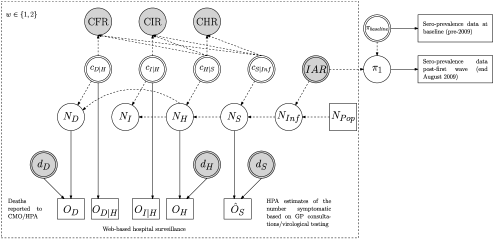
Figure 1: Schematic DAG for the severity model, first two waves, for one age group.

5 The severity model in England

The model used in Presanis et al. (2011b) for the first two waves of infection in England is described in the next section. Two alternative methods of modelling the third wave of infection are then given: (a) a two-stage approach where posterior distributions from the second wave model are used to inform prior distributions for some of the conditional probabilities in the third wave; and (b) a one-stage approach where all three waves are modelled simultaneously, with the third wave conditional probabilities parameterised in terms of the corresponding second wave probabilities.

5.1 First & second waves

Figure 1 is a schematic Directed Acyclic Graph (DAG) displaying the relationship between parameters and data in the model for severity in the first two waves in England [Presanis et al. (2011b)]. The figure displays one generic example age group, with the $a$ and $w$ indices left out for simplicity. Parameters are denoted by circles and data by rectangles. The dashed rectangle represents repetition over the two waves $w\in\{1,2\}$. Double circles are basic parameters which are assigned prior distributions, either vague or informative, and filled light grey circles denote the key parameters (both basic and functional) we wish to estimate. Dashed arrows denote functional relationships, for example, the definition of each number $N_{w,a,l}=c_{w,a,l|\lambda}\times N_{w,a,\lambda}$ or equations (4.1) and (4.1). Solid arrows represent distributional assumptions, for example, that an observation is Binomially distributed.

5.1.1 Prior distribution

Independently for each age group, a vague$\operatorname{Dirichlet}(1,1,1)$ prior distribution is given to the infection attack rate,$\mathit{IAR}_{w,a}$, in each of the two waves, together with the remaining fraction of the population, comprising those either uninfected in the first two waves or with some degree of immunity at baseline:

$$\Biggl{(}\mathit{IAR}_{1,a},\mathit{IAR}_{2,a},1-\sum_{w=1}^{2}\mathit{IAR}_{w,a}\Biggr{)}\sim\operatorname{Dirich}(1,1,1).$$

The three proportions are therefore constrained a priori to sum to 1 and to lie between 0 and 1. This parameterisation assumes each infected individual was infected in only a single wave. The remaining priors are either Uniform or Beta distributions, with full details given in Section 2.2 of the supplementary material [Presanis et al. (2014)].

5.1.2 Likelihood

The likelihood is a product of binomial and log-normal contributions, as detailed in the following.

Infections

The sero-prevalence data [source (iii) of Section 2] consist of the number of samples testing positive for pandemic A/H1N1 antibodies, both before and after the first wave. They are realisations of two binomial distributions and provide information on the corresponding prevalences at the two time points. The difference in these two prevalences informs the infection attack rate in the first wave, via the functional relationship $\pi_{1,a}=\pi_{\mathrm{baseline},a}+\mathit{IAR}_{1,a}$ (Figure 1). The post-second wave sero-prevalence data were not used initially, as some samples taken after the vaccination campaign had begun were likely to test positive due to vaccination rather than infection. A lack of information on the vaccination status of individuals in the sample, together with concerns that individuals in the sample may have been more likely than the general population to be at risk of infection, due to pre-existing conditions, and therefore to be vaccinated [Miller et al. (2010), Bird (2010)], precluded the use of the data without further work to address these challenges.

Symptomatic infections

The estimates $\hat{O}_{w,a,S}$ (Figure 1) of the number symptomatic from the HPA (source (ii), Section 1.1.2 of the supplementary material [Presanis et al. (2014)]) are assumed to be log-normally distributed, with a mean that (on the original scale) is drawn from a binomial distribution with size parameter $N_{w,a,S}$ and probability parameter given by the detection probability $d_{w,a,S}$. This parameterisation reflects the belief that the HPA estimates are underestimates of the number symptomatic $N_{w,a,S}$.

Hospitalisations and deaths

The observed hospitalisations $O_{w,a,H}$ anddeaths $O_{w,a,D}$ [sources (iv) and (v), resp., see also Figure 1] are binomial realisations, with size parameters $N_{w,a,l},l\in\{H,D\}$ and probability parameters given by their respective (wave- but not age-specific) detection probabilities $d_{w,\ell}$. Amongst observed hospitalisations for whom we have information on final outcomes [a subset of source (iv)], the observed ICU admissions and deaths are realisations of binomial distributions with probability parameters given by the conditional probabilities $c_{w,a,I|H}$ and $c_{w,a,D|H}$, respectively (Figure 1). Fuller details of the model are given in Section 2 of the supplementary material [Presanis et al. (2014)].

5.2 The third wave: A two-stage approach

The changes in surveillance sources available during the third wave, particularly the smaller sample sizes and coarser age aggregation, resulted in the data providing less direct information on the parameters than in the first two waves. To ensure identifiability of all parameters, informative prior distributions were employed for some parameters. The darker grey circles in Figure 2, a DAG of the third wave model, denote these parameters, with Beta prior distributions chosen to reflect the posterior distributions of the equivalent second wave parameters (see Table 15 of the supplementary material [Presanis et al. (2014)]). The changes also entailed two smaller submodels, one for the data on ICU patients with suspected pandemic A/H1N1 infection and one for general practice (GP) consultation and positivity data, the results of which are incorporated into the third wave severity model as likelihood terms (see below for more detail).

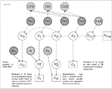
Figure 2: Schematic DAG for the severity model, third wave, for one age group.

Infections. The infection attack rate again has a Dirichlet prior over the three waves, but it is now more informative:

$$(\pi_{2,a},\mathit{IAR}_{3,a},1-\pi_{2,a}-\mathit{IAR}_{3,a})\sim\operatorname{Dirich}(2x_{a}/y_{a},1,1),$$

where $\pi_{2,a}$ is the proportion either with antibodies at baseline or infected during one of the first two waves, that is, the post-second wave antibody prevalence. For each age group $a$, $x_{a}$ and $y_{a}$ are chosen such that a $\operatorname{Beta}(x_{a},\break y_{a})$ distribution approximates the marginal posterior distribution of $\pi_{2,a}$ derived from the model of Section 5.1. The choice of Dirichlet parameters allows the prior mean for $\pi_{2,a}$ to reflect the posterior mean from Section 5.1, but gives greater prior uncertainty than the corresponding posterior.

Symptomatic infections. As the HPA did not produce estimates of the number symptomatic during the third wave, data on ILI consultations and virological positivity from an alternative primary care sentinel surveillance system ([Fleming (1999)]; see Section 1.2.1 of the supplementary material [Presanis et al. (2014)]) were used to estimate the number symptomatic, before incorporating this estimate into the severity model. A log-linear regression of the ILI consultation data on time and age was fitted jointly with a logistic regression of the positivity data on time and age [cf. Birrell et al. (2011)]. A negative binomial likelihood was assumed for the consultation data and a binomial likelihood for the positivity data. The number symptomatic due to the pandemic A/H1N1 strain was then estimated as the sum over weeks of the product of the expected consultation rate and the expected proportion positive for pandemic A/H1N1, adjusted for the proportion of symptomatic patients who contact primary care. The resulting posterior mean ($\hat{O}^{\prime}_{3,a,S}$) and standard deviation ($\sigma^{\prime}_{3,a,S}$) of the logarithm of the number symptomatic are incorporated into the likelihood of the third wave severity model as a normal term:

$$\hat{O}^{\prime}_{3,a,S}\sim N\bigl{(}\log(N_{3,a,S}),\sigma^{\prime 2}_{3,a,S}\bigr{)}$$

(see Section 3.1 of the supplementary material [Presanis et al. (2014)] for details).

Hospitalisations. The hospitalisation data for the third wave (source (vi), Section 1.2.2 of the supplementary material [Presanis et al. (2014)]) come from a sentinel system. The observed number of hospitalisations therefore provides a lower bound for the number of hospitalisations, contributing to the total likelihood as a binomial component with probability parameter given by the (non-age specific) detection probability $d_{3,H}$. Recall that these data are available at a coarser age aggregation than in the first two waves. The size parameter is therefore a functional parameter $N^{*}_{3,b,H}=\sum_{a\in A_{b,H}}N_{3,a,H}$ that is a sum over the appropriate age groups $a\in A_{b,H}$, where $A_{b,H}$ are sets describing the mapping from the coarser age groups $b$ to the severity model age groups $a$.

ICU admissions. The extra information on suspected patients present in ICU (source (vii), Section 1.2.3 of the supplementary material [Presanis et al. (2014)]) are modelled as a bivariate immigration-death process to represent movement in and out of ICU. This process is combined with the positivity data of source (viii) to estimate the cumulative number of confirmed pandemic A/H1N1 incident cases admitted to ICU during the third wave (Section 4 of the supplementary material [Presanis et al. (2014)]). The resulting posterior mean (standard deviation) of the logarithm of the cumulative ICU admissions, $\hat{O}^{\prime}_{3,b,I}(\sigma^{\prime}_{3,b,I})$, are incorporated in the likelihood for the third wave severity model as normally distributed:

$$\hat{O}^{\prime}_{3,b,I}\sim N\bigl{(}\log\bigl{(}N^{*}_{3,b,I}\bigr{)},\sigma^{\prime 2}_{3,b,I}\bigr{)},$$

where $b$ denotes the age groups available for the suspected ICU data (two groups: children and adults). As with the hospitalisation data, the $N^{*}_{3,b,I}=\sum_{a\in A_{b,I}}N^{*}_{3,a,I}$ are sums over the appropriate age groups. The number $N^{*}_{w,a,I}$ is still a lower bound for the cumulative number of ICU admissions over the third wave, since the data of source (vii) cover only a portion of the time of the third wave: this is expressed as having a binomial distribution with size parameter $N_{w,a,I}$ and probability parameter given by the age-constant detection probability $d_{w,I}$.

Deaths. Finally, the observed deaths are again binomially distributed, as in the first two waves. Full details of the changes to model the third wave are given in Section 3 of the supplementary material [Presanis et al. (2014)].

5.3 Modelling all three waves simultaneously

Modelling the three waves of infection in two stages enables the use of the posterior distributions of case-severity in the second wave as prior distributions in the third wave analysis. However, a two-stage approach does not allow estimation of the posterior probability of a change in severity occurring over waves. To do so requires modelling all three waves simultaneously, as if we had not seen any of the data until the end of the third wave.

A joint model for all three waves implies different assumptions from the two-stage approach. First, the prior distribution for the infection attack rates in each wave is assumed again to be diffuse:

$$\Biggl{(}\mathit{IAR}_{1,a},\mathit{IAR}_{2,a},\mathit{IAR}_{3,a},1-\sum_{w=1}^{3}\mathit{IAR}_{w,a}\Biggr{)}\sim\operatorname{Dirich}(1,1,1,1).$$

Here, the remaining fraction of the population $1-\sum_{w=1}^{3}\mathit{IAR}_{w,a}$ comprises both those with antibodies at baseline (pre-pandemic) and those remaining uninfected by the end of the third wave.

The proportion symptomatic, $c_{S|\mathit{Inf}}$, is now constrained to be equal across all three waves and all age groups, instead of its third wave prior being informed by its second wave posterior distribution. Likewise, the three conditional probabilities $\mathit{sCHR}_{w,a}=c_{w,a,H|S},c_{w,a,I|H}$ and $c_{w,a,D|H}$ for $w=3$ are no longer given prior distributions based on second wave posterior distributions, but are parameterised in terms of their corresponding second wave conditional probabilities:

$$\operatorname{logit}(c_{3,a,l|\lambda}) \sim N\bigl{(}\operatorname{logit}(c_{2,a,l|\lambda}),\tau^{2}_{l|\lambda}\bigr{)}$$ (3)

$$\mbox{for each $(l|\lambda)\in\bigl{\{}(H|S),(I|H),(D|H)\bigr{\}}$},$$

$$\tau_{l|\lambda} \sim \operatorname{Unif}[0,1].$$

A value of $\tau=1$ for the standard deviations would imply that the odds ratios of the third compared to the second wave probabilities lie between 0.14 and 7.10. A value of $\tau=0$ would imply an odds ratio of 1, that is, equality of the conditional probabilities: $c_{3,a,l|\lambda}=c_{2,a,l|\lambda}$.

All other aspects of the joint model for all three waves are as in the separate first/second and third wave models of Sections 5.1 and 5.2, respectively.

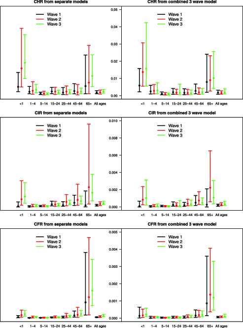
Figure 3: $\mathit{CHR},\mathit{CIR}$ and $\mathit{CFR}$ by age, wave and model. Note the different scales on the $y$-axes.

Figure 4: Infection attack rate by age, wave and model.

6 Results

Results from the model for the first two waves, given in full in Presanis et al. (2011b), suggest a mild pandemic, characterised by case-severity risks increasing between the two waves. From the analysis of data from the third wave, Figures 3 and 4 show the posterior medians and $95\%$ credible intervals for the case-severity risks and infection attack rates, respectively, by age, wave and model. Although there are some differences between the two-stage models (left-hand sides of the figures) and the combined three-wave model (right-hand sides), the conclusions are broadly similar. There is a clear “u”-shape to the age distribution of the case-severity risks (Figure 3) in all three waves, with the youngest and oldest age groups having the highest probabilities of experiencing severe events, but also the most uncertainty in the estimates. The age distribution of the infection attack rates (Figure 4), on the other hand, is convex, with school-age children having the highest probability of being infected in the first two waves, though not the third.

The joint three-wave model allows estimation of the posterior probabilities of increases across waves in either the attack rates or the case-severity risks (Table 1). Across waves, there is some evidence of a shift in the age distribution of the infection attack rates, with posterior probabilities $p\geq 0.85$ of an increase from the second to third waves seen in adults and the very young, but not in school-age children (posterior probability $p=0.13$).

At first glance, the estimates averaged over the age groups (Table 1) suggest the case-severity risks have increased over all three waves. The posterior probabilities of a rise across waves of the $\mathit{CIR}$ and $\mathit{CFR}$ are all greater than $73\%$. However, closer scrutiny of the age-specific estimates shows this increase does not occur consistently in every age group and wave. There is stronger evidence of a rise in ICU admission and fatalities from the first to second waves than from the second to third. The pattern is less clear in the case-hospitalisation risks.

Table 1: Posterior probabilities, by age, that the $\mathit{IAR},\mathit{CHR},\mathit{CIR},\mathit{CFR},c_{I|H}$ and $c_{D|H}$ are greater in (a) wave 2 vs wave 1, (b) wave 3 vs wave 2, and (c) wave 3 vs wave 1

	Age	$\bolds{\operatorname{Pr}(W2>W1)}$	$\bolds{\operatorname{Pr}(W3>W2)}$	$\bolds{\operatorname{Pr}(W3>W1)}$
$\mathit{IAR}$	$<$1	$19\%$	$87\%$	$71\%$
	1–4	$96\%$	$85\%$	$99\%$
	5–14	$99\%$	$13\%$	$77\%$
	15–24	$94\%$	$96\%$	$100\%$
	25–44	$96\%$	$100\%$	$100\%$
	45–64	$100\%$	$99\%$	$100\%$
	65$+$	$95\%$	$99\%$	$100\%$
	All ages	$100\%$	$99\%$	$100\%$
$\mathit{CHR}$	$<$1	$96\%$	$62\%$	$95\%$
	1–4	$60\%$	$57\%$	$64\%$
	5–14	$26\%$	$27\%$	$13\%$
	15–24	$37\%$	$48\%$	$39\%$
	25–44	$47\%$	$36\%$	$38\%$
	45–64	$19\%$	$52\%$	$24\%$
	65$+$	$60\%$	$63\%$	$68\%$
	All ages	$30\%$	$79\%$	$54\%$
$\mathit{CIR}$	$<$1	$98\%$	$62\%$	$97\%$
	1–4	$86\%$	$58\%$	$86\%$
	5–14	$43\%$	$34\%$	$31\%$
	15–24	$34\%$	$31\%$	$27\%$
	25–44	$91\%$	$36\%$	$82\%$
	45–64	$80\%$	$14\%$	$50\%$
	65$+$	$98\%$	$11\%$	$89\%$
	All ages	$90\%$	$73\%$	$95\%$
$\mathit{CFR}$	$<$1	$58\%$	$69\%$	$70\%$
	1–4	$74\%$	$64\%$	$80\%$
	5–14	$38\%$	$82\%$	$66\%$
	15–24	$60\%$	$24\%$	$41\%$
	25–44	$86\%$	$35\%$	$77\%$
	45–64	$61\%$	$52\%$	$61\%$
	65$+$	$74\%$	$40\%$	$67\%$
	All ages	$76\%$	$90\%$	$93\%$
$c_{I|H}$	$<$1	$90\%$	$54\%$	$90\%$
	1–4	$85\%$	$54\%$	$85\%$
	5–14	$65\%$	$53\%$	$66\%$
	15–24	$39\%$	$32\%$	$28\%$
	25–44	$100\%$	$43\%$	$99\%$
	45–64	$100\%$	$0\%$	$93\%$
	65$+$	$99\%$	$1\%$	$87\%$
	All ages	$100\%$	$35\%$	$100\%$

Table 1: (Continued)

	Age	$\bolds{\operatorname{Pr}(W2>W1)}$	$\bolds{\operatorname{Pr}(W3>W2)}$	$\bolds{\operatorname{Pr}(W3>W1)}$
$c_{D|H}$	$<$1	$26\%$	$62\%$	$31\%$
	1–4	$71\%$	$61\%$	$76\%$
	5–14	$52\%$	$96\%$	$93\%$
	15–24	$69\%$	$20\%$	$46\%$
	25–44	$94\%$	$43\%$	$91\%$
	45–64	$90\%$	$51\%$	$89\%$
	65$+$	$72\%$	$20\%$	$54\%$
	All ages	$97\%$	$85\%$	$98\%$

The reason for the pattern of increase in the $\mathit{CIR}$ and $\mathit{CFR}$ over waves is not immediately apparent without further investigation. Three possible hypotheses are as follows: (a) that the increase is due to the age shift in the infection attack rate away from school-age children toward adults across waves; (b) that the lack of third wave data and consequent parameterisation of some of the third wave conditional probabilities in terms of the corresponding second wave probabilities [equation (3)] results in the attenuated change in severity from the second to third wave; and/or (c) that unaccounted differences in the representativeness of the different surveillance systems used in the third wave compared to the first two may have an effect on the estimated severity. These possibilities are not mutually exclusive and the extent to which the estimated severity is reliant on each is unknown.

6.1 Sensitivity analyses

The potential for unaccounted biases in the sero-prevalence data (Sections 2 and 5.1.2), as well as the belief that the HPA case estimates represented underestimates, prompted several sensitivity analyses to further assess the uncertainty in the infection attack rates in the first two waves. Sensitivity to the choice of data informing the denominators (the infection attack rate $\mathit{IAR}_{w,a}$ or the number of symptomatic infections $N_{w,a,S}$) and to the prior distribution of $\mathit{IAR}_{w,a}$ was assessed. Specifically, four models with different data informing $\mathit{IAR}_{w,a}$ and $N_{w,a,S}$ were considered: [1.]

using the HPA case estimates to inform $N_{w,a,S}$, assuming they do so unbiasedly in the first two waves (i.e., with $d_{w,a,S}=1$), and using no sero-prevalence data;

the model presented here and in Presanis et al. (2011b), assuming the HPA case estimates are biased downwards and using only the baseline and post-first wave sero-prevalence data;

as in model 2, but using all the sero-prevalence data (up to post-second wave) of Table 5 of Section 1.1.3 of the supplementary material [Presanis et al. (2014)], assuming the HPA case estimates are biased downwards in both waves; and

as in model 3, but assuming the sero-prevalence data are biased upwards and the HPA case estimates are biased downwards. Analyses using models 1 and 2 were then repeated using three different prior distributions for the infection attack rate: [a.]

$\operatorname{Dirichlet}(2,2,6)$, allowing the total attack rate over the two waves to be a priori $0.4$ on average, with $95\%$ prior mass in the interval (0.1–0.7), and with a $1:1$ ratio between the two waves;

$\operatorname{Dirichlet}(2.67,1.33,6)$, allowing again a prior total attack rate of 0.4 (0.1–0.7), but with a $2\dvtx 1$ ratio between waves;

$\operatorname{Dirichlet}(1.33,2.67,6)$, allowing a prior total attack rate of 0.4 (0.1–0.7), with a $1:2$ ratio between waves.

The choice of informative priors is motivated by the total attack rates in prior pandemics, with the prior uncertainty still relatively large. Jackson, Vynnycky and Mangtani (2010) found susceptible attack rates (i.e., proportion of susceptibles infected, as opposed to proportion of the total population) of between $19$ and $58\%$ in the first wave of the 1968–1969 pandemic, compared to between $15$ and $50\%$ in the second, which motivates prior (b). This prior may in fact be sceptical for the 2009 pandemic, as instead of a $2:1$ ratio between waves, the HPA case estimates and the severe data suggest the ratio was at least $1:1$, if not $1:2$ or greater. However, this ratio may vary by both age and region, with London in particular experiencing a somewhat different epidemic to the rest of the country [Birrell et al. (2011)]. Prior (c) therefore allows for the converse, with a greater second wave than first.

The sensitivity analyses to the choice of prior distribution of the infection attack rate in the first two waves suggest the key messages from Presanis et al. (2011b) are robust to the choice of prior distribution. Results were less robust to the choice of denominator data included in the model. The inclusion of the post-second wave sero-prevalence data suggested a higher infection attack rate [28.4% (26.0–30.8%)] than the baseline analysis [11.2% (7.4–18.9%)], with a corresponding lower case-fatality risk in the second wave [0.0027% (0.0024–0.0031%) compared to 0.009% (0.004–0.014%)]. Full details of these sensitivity analyses are given in Section 5 of the supplementary material [Presanis et al. (2014)]. Recall (Section 5.1.2) that the samples tested post-second wave and before and after the third wave [Hoschler et al. (2012)] may overrepresent individuals at higher risk of infection and vaccination. The observed sero-prevalence in these samples may therefore suggest a higher infection attack rate than truly occurred. Further work to obtain background information on individuals in the samples, and therefore to account for sampling biases, is underway, prompted in part by the results of these sensitivity analyses.

In the third wave, a sensitivity analysis to the set of virological positivity data used was performed (Sections 1.2.1 and 3.1 of the supplementary material [Presanis et al. (2014)]). The main analysis used the full positivity data, with the results of the Bayesian joint regression model of the positivity and primary care consultation data (Table 13 of the supplementary material) incorporated into the combined 3-wave model as shown in Figure 2 and Section 3.1 of the supplementary material. The sensitivity analysis employed instead a set of virological positivity data restricted to tests made on swabs that were collected within 5 days of an ILI consultation, with corresponding results from the joint regression model in Table 14 of the supplementary material. The results from including the two alternative sets of estimates from the joint regression model into the combined 3-wave model are compared in Figures 5 and 6.

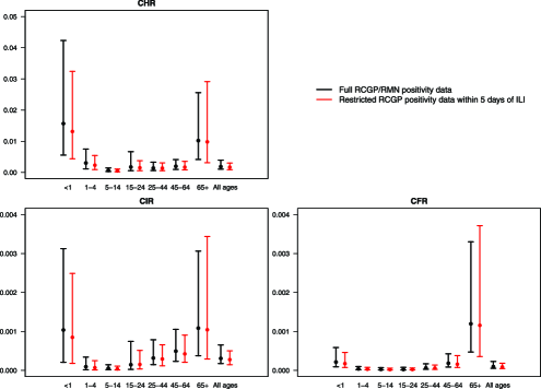
Figure 5: Third wave $\mathit{CHR},\mathit{CIR}$ and $\mathit{CFR}$ from the combined model, by age and source of positivity data. Note the different scales on the $y$-axes.

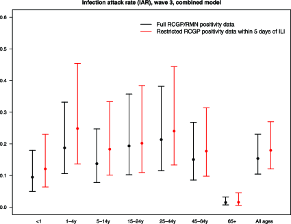
Figure 6: Third wave infection attack rate from the combined model, by age and positivity data set used.

The general conclusions about the age distribution of the case-severity risks and infection attack rate in the third wave are unchanged by the use of the restricted positivity data. The restricted data do imply a slightly higher and more uncertain attack rate in each age group (Figure 6), due to the higher observed positivity and smaller sample sizes. Correspondingly, the case-severity risks are slightly lower in each age group in the sensitivity analysis (Figure 5), but the greater uncertainty in the denominator does not seem to translate directly into greater uncertainty in the risks.

7 Discussion

We have extended and further developed a Bayesian evidence synthesis model [Presanis et al. (2011b)] to characterise and estimate the severity of the 2009 pandemic A/H1N1 strain of influenza in the three waves of infection experienced in England. The model has been adapted to account for changes in the surveillance data available over the course of the three waves, considering two approaches: (a) a two-stage approach, using posterior distributions from the model for the first two waves to inform prior distributions for the third wave analysis; and (b) modelling all three waves simultaneously, accounting for the reduction in available data by parameterising the third wave severity parameters in terms of the corresponding second wave parameters. Both approaches have resulted in broadly the same three key conclusions: [1.]

The age distribution in case-severity risks is “u”-shaped, implying children aged less than a year and older adults have highest severity, although their estimates are also the most uncertain. This pattern is consistent with the increasing severity with age seen in other countries during the 2009 pandemic [Presanis et al. (2009), Wu et al. (2010), Sypsa et al. (2011), Shubin et al. (2013), Wong et al. (2013)], where in each of these analyses, the authors did not distinguish between children under 1 year of age and those aged 1–4. The pattern is also consistent with global relative risks by age of severe events compared to the general population estimated by Van Kerkhove et al. (2011).

The age distribution of the infection attack rate changes over waves, with school-age children most affected in the first two waves and an increase in the attack rate in adults aged 25 and older from the second to third waves.

When averaged over all ages, severity in those infected appears to increase over the three waves. The changing age distribution and apparent increase in severity over waves is consistent with estimates from the two pandemic waves experienced by other countries [Yang et al. (2011), Truelove et al. (2011), Shubin et al. (2013)].

It is important to note that the estimates presented here do not account for risk factors for severe influenza, nor for vaccination status nor for other preventive measures, such as social distancing, which might have an effect on severity. Both the joint regression model of virological positivity and GP consultation and the full severity model would require further development to account for these factors and to be able to use the second and third wave serology data accounting for sampling biases. Assessment of the effect on estimates of assumptions—such as that of no influenza-related deaths occurring outside of hospital or the parameterisation of the third wave in terms of the second wave in the combined analysis—is also key. The possible effect of any differences in representativeness of the various surveillance systems in the third compared to the first two waves is an issue for further investigation. The sample sizes and prior distributions chosen do not provide enough information to enable convergence of the MCMC algorithm for the severity model when taking the number of infections $N_{w,a,l}$ to be a Binomial realisation from the number at a less severe level $\lambda$. This lack of convergence implies there may be too much uncertainty to allow identifiability of the model in this case, prompting instead the mean assumption $N_{w,a,l}=c_{w,a,l|\lambda}\times N_{w,a,\lambda}$. Another area for future investigation is to assess how informative the priors are required to be or how large sample sizes need to be to enable convergence when the $N_{w,a,\lambda}$ are stochastic.

Despite these challenges, our Bayesian evidence synthesis approach has allowed us to draw important public health conclusions, not only in characterising the severity of the 2009 pandemic, but also in shaping future research. The sensitivity analyses showed the severity estimates were robust to prior assumptions about the infection attack rate, but less robust to the choice of data to include in informing the attack rate. Although the magnitude of the severity estimates varied, the conclusions of a “u”-shaped age distribution to severity and an apparent increase in severity over waves were nevertheless robust. The sensitivity of the results has, furthermore, contributed to the initiation of a project to obtain further data to better understand the potential sampling bias in the sero-prevalence data [Laurie et al. (2013)].

The evidence synthesis framework has also given us the flexibility to account for biases, using prior information on parameters representing the biases, for example. Bias modelling has been an integral part of the model development, inference and criticism cycle, as have the sensitivity analyses. It is important, in any analysis, to understand the contribution of each item of evidence, whether in the form of model structure, prior distribution or data, in driving inferences. It is particularly crucial when an analysis relies on informative priors for identifiability, as is the case here. Another key aspect of model criticism in an evidence synthesis is to assess the consistency of the various data sources, not only with each other, but also with the model structure. It is possible, and indeed common, in syntheses of multiple sources of evidence to find both that some parameters are only barely identified by the data and that other parameters are informed indirectly by more than one data item. In the latter case, there is clearly potential for different sources of data to conflict, providing inconsistent evidence on a particular parameter [Lu and Ades (2006), Sweeting et al. (2008), Presanis et al. (2008)]. Such conflicts need to be detected, measured, understood and resolved. Conflict diagnostics, in the form of cross-validatory posterior prediction, for the first wave confirm the inconsistency between the serology data and the HPA estimates of the number symptomatic if taken at face value [Presanis et al. (2013)]. In our main analysis, we addressed the conflict by incorporating a bias parameter for the HPA estimates, whereas in the sensitivity analyses, we also considered a bias parameter for the serology data. Further preliminary work on measuring conflict seems to confirm the suggestion of the sensitivity analyses that the severe end data does indeed conflict with the evidence on the attack rates. Given the uncertainties in the attack rates, understanding and resolving this conflict is an important next step. The iterative process of fitting, criticising and further developing an evidence synthesis model to address conflicts, as we have done and are continuing to do here, leads automatically to internal consistency. By contrast, external validation is much more challenging in an evidence synthesis framework. As already noted, due to identifiability issues common to evidence syntheses, it is rare to find external data against which to validate—such data are instead used in the synthesis.

Despite these challenges, an evidence synthesis using a complex probabilistic model provides a powerful approach to estimating influenza severity when the available evidence comes from multiple sources that are incomplete and biased. The embedding of a “pyramid” approach to severity estimation within an evidence synthesis framework, as presented here, is easily adapted to other contexts, both within epidemiology, where many diseases may be observed at different levels of severity or diagnosis, and in other fields where observation occurs at different levels, for example, quality control or ecology.

References

- Ades and Sutton (2006) {barticle}[mr] \bauthor\bsnmAdes, \bfnmA. E.\binitsA. E. and \bauthor\bsnmSutton, \bfnmA. J.\binitsA. J. (\byear2006). \btitleMultiparameter evidence synthesis in epidemiology and medical decision-making: Current approaches. \bjournalJ. Roy. Statist. Soc. Ser. A \bvolume169 \bpages5–35. \biddoi=10.1111/j.1467-985X.2005.00377.x, issn=0964-1998, mr=2222010 \bptokimsref\endbibitem
- Albert et al. (2011) {barticle}[author] \bauthor\bsnmAlbert, \bfnmIsabelle\binitsI., \bauthor\bsnmEspié, \bfnmEmmanuelle\binitsE., \bauthor\bparticlede \bsnmValk, \bfnmHenriette\binitsH. and \bauthor\bsnmDenis, \bfnmJean-Baptiste B.\binitsJ.-B. B. (\byear2011). \btitleA Bayesian evidence synthesis for estimating campylobacteriosis prevalence. \bjournalRisk Analysis \bvolume31 \bpages1141–1155. \bptokimsref\endbibitem
- Bird (2010) {barticle}[author] \bauthor\bsnmBird, \bfnmSheila M.\binitsS. M. (\byear2010). \btitleLike-with-like comparisons? \bjournalThe Lancet \bvolume376 \bpages684+. \bptokimsref\endbibitem
- Birrell et al. (2011) {barticle}[author] \bauthor\bsnmBirrell, \bfnmPaul J.\binitsP. J., \bauthor\bsnmKetsetzis, \bfnmGeorgios\binitsG., \bauthor\bsnmGay, \bfnmNigel J.\binitsN. J., \bauthor\bsnmCooper, \bfnmBen S.\binitsB. S., \bauthor\bsnmPresanis, \bfnmAnne M.\binitsA. M., \bauthor\bsnmHarris, \bfnmRoss J.\binitsR. J., \bauthor\bsnmCharlett, \bfnmAndré\binitsA., \bauthor\bsnmZhang, \bfnmXu-Sheng\binitsX.-S., \bauthor\bsnmWhite, \bfnmPeter J.\binitsP. J., \bauthor\bsnmPebody, \bfnmRichard G.\binitsR. G. and \bauthor\bsnmDe Angelis, \bfnmDaniela\binitsD. (\byear2011). \btitleBayesian modeling to unmask and predict influenza A/H1N1pdm dynamics in London. \bjournalProc. Natl. Acad. Sci. USA \bvolume108 \bpages18238–18243. \bptokimsref\endbibitem
- Box (1980) {barticle}[mr] \bauthor\bsnmBox, \bfnmGeorge E. P.\binitsG. E. P. (\byear1980). \btitleSampling and Bayes’ inference in scientific modelling and robustness. \bjournalJ. Roy. Statist. Soc. Ser. A \bvolume143 \bpages383–430. \biddoi=10.2307/2982063, issn=0035-9238, mr=0603745 \bptnotecheck related \bptokimsref\endbibitem
- Brooks and Gelman (1998) {barticle}[mr] \bauthor\bsnmBrooks, \bfnmStephen P.\binitsS. P. and \bauthor\bsnmGelman, \bfnmAndrew\binitsA. (\byear1998). \btitleGeneral methods for monitoring convergence of iterative simulations. \bjournalJ. Comput. Graph. Statist. \bvolume7 \bpages434–455. \biddoi=10.2307/1390675, issn=1061-8600, mr=1665662 \bptokimsref\endbibitem
- Campbell et al. (2011) {barticle}[author] \bauthor\bsnmCampbell, \bfnmC. N. J.\binitsC. N. J., \bauthor\bsnmMytton, \bfnmO. T.\binitsO. T., \bauthor\bsnmMcLean, \bfnmE. M.\binitsE. M., \bauthor\bsnmRutter, \bfnmP. D.\binitsP. D., \bauthor\bsnmPebody, \bfnmR. G.\binitsR. G., \bauthor\bsnmSachedina, \bfnmN.\binitsN., \bauthor\bsnmWhite, \bfnmP. J.\binitsP. J., \bauthor\bsnmHawkins, \bfnmC.\binitsC., \bauthor\bsnmEvans, \bfnmB.\binitsB., \bauthor\bsnmWaight, \bfnmP. A.\binitsP. A., \bauthor\bsnmEllis, \bfnmJ.\binitsJ., \bauthor\bsnmBermingham, \bfnmA.\binitsA., \bauthor\bsnmDonaldson, \bfnmL. J.\binitsL. J. and \bauthor\bsnmCatchpole, \bfnmM.\binitsM. (\byear2011). \btitleHospitalization in two waves of pandemic influenza A(H1N1) in England. \bjournalEpidemiology and Infection \bvolume139 \bpages1560–1569. \bptokimsref\endbibitem
- Department of Health (2011) {bmisc}[author] \borganizationDepartment of Health (\byear2011). \bhowpublishedDepartment of Health Winter Watch. Accessed 25/02/2011. \bptokimsref\endbibitem
- Donaldson et al. (2009) {barticle}[pbm] \bauthor\bsnmDonaldson, \bfnmLiam J.\binitsL. J., \bauthor\bsnmRutter, \bfnmPaul D.\binitsP. D., \bauthor\bsnmEllis, \bfnmBenjamin M.\binitsB. M., \bauthor\bsnmGreaves, \bfnmFelix E. C.\binitsF. E. C., \bauthor\bsnmMytton, \bfnmOliver T.\binitsO. T., \bauthor\bsnmPebody, \bfnmRichard G.\binitsR. G. and \bauthor\bsnmYardley, \bfnmIain E.\binitsI. E. (\byear2009). \btitleMortality from pandemic A/H1N1 2009 influenza in England: Public health surveillance study. \bjournalBMJ \bvolume339 \bpagesb5213. \bidissn=1756-1833, pmcid=2791802, pmid=20007665 \bptokimsref\endbibitem
- Eddy, Hasselblad and Shachter (1992) {bbook}[author] \bauthor\bsnmEddy, \bfnmDavid M.\binitsD. M., \bauthor\bsnmHasselblad, \bfnmVic\binitsV. and \bauthor\bsnmShachter, \bfnmRoss\binitsR. (\byear1992). \btitleMeta-Analysis by the Confidence Profile Method. \bpublisherAcademic Press, \blocationBoston, MA. \bptokimsref\endbibitem
- Fleming (1999) {barticle}[author] \bauthor\bsnmFleming, \bfnmD. M.\binitsD. M. (\byear1999). \btitleWeekly returns service of the royal college of general practitioners. \bjournalCommunicable Disease and Public Health / PHLS \bvolume2 \bpages96–100. \bptokimsref\endbibitem
- Garske et al. (2009) {barticle}[pbm] \bauthor\bsnmGarske, \bfnmTini\binitsT., \bauthor\bsnmLegrand, \bfnmJudith\binitsJ., \bauthor\bsnmDonnelly, \bfnmChristl A.\binitsC. A., \bauthor\bsnmWard, \bfnmHelen\binitsH., \bauthor\bsnmCauchemez, \bfnmSimon\binitsS., \bauthor\bsnmFraser, \bfnmChristophe\binitsC., \bauthor\bsnmFerguson, \bfnmNeil M.\binitsN. M. and \bauthor\bsnmGhani, \bfnmAzra C.\binitsA. C. (\byear2009). \btitleAssessing the severity of the novel influenza A/H1N1 pandemic. \bjournalBMJ \bvolume339 \bpagesb2840. \bidissn=1756-1833, pmid=19602714 \bptokimsref\endbibitem
- Goubar et al. (2008) {barticle}[mr] \bauthor\bsnmGoubar, \bfnmA.\binitsA., \bauthor\bsnmAdes, \bfnmA. E.\binitsA. E., \bauthor\bsnmDe Angelis, \bfnmD.\binitsD., \bauthor\bsnmMcGarrigle, \bfnmC. A.\binitsC. A., \bauthor\bsnmMercer, \bfnmC. H.\binitsC. H., \bauthor\bsnmTookey, \bfnmP. A.\binitsP. A., \bauthor\bsnmFenton, \bfnmK.\binitsK. and \bauthor\bsnmGill, \bfnmO. N.\binitsO. N. (\byear2008). \btitleEstimates of human immunodeficiency virus prevalence and proportion diagnosed based on Bayesian multiparameter synthesis of surveillance data. \bjournalJ. Roy. Statist. Soc. Ser. A \bvolume171 \bpages541–580. \biddoi=10.1111/j.1467-985X.2007.00537.x, issn=0964-1998, mr=2432503 \bptokimsref\endbibitem
- Hardelid et al. (2011) {barticle}[author] \bauthor\bsnmHardelid, \bfnmP.\binitsP., \bauthor\bsnmAndrews, \bfnmN. J.\binitsN. J., \bauthor\bsnmHoschler, \bfnmK.\binitsK., \bauthor\bsnmStanford, \bfnmE.\binitsE., \bauthor\bsnmBaguelin, \bfnmM.\binitsM., \bauthor\bsnmWaight, \bfnmP. A.\binitsP. A., \bauthor\bsnmZambon, \bfnmM.\binitsM. and \bauthor\bsnmMiller, \bfnmE.\binitsE. (\byear2011). \btitleAssessment of baseline age-specific antibody prevalence and incidence of infection to novel influenza A/H1N1 2009. \bjournalHealth Technology Assessment \bvolume14 \bpages115–192. \bptokimsref\endbibitem
- Health Protection Agency (2010) {bmisc}[author] \borganizationHealth Protection Agency (\byear2010). \bhowpublishedEpidemiological report of pandemic (H1N1) 2009 in the UK. Technical report, Health Protection Agency. \bptokimsref\endbibitem
- Health Protection Agency, Health Protection Scotland, Communicable Disease Surveillance Centre Northern Ireland and National Public Health Service for Wales (2009) {bmisc}[author] \borganizationHealth Protection Agency, Health Protection Scotland, Communicable Disease Surveillance Centre Northern Ireland and National Public Health Service for Wales (\byear2009). \bhowpublishedFirst Few Hundred (FF100) Project: Epidemiological Protocols for Comprehensive Assessment of Early Swine Influenza Cases in the United Kingdom Technical report, Health Protection Agency. \bptokimsref\endbibitem
- Hoschler et al. (2012) {barticle}[pbm] \bauthor\bsnmHoschler, \bfnmKatja\binitsK., \bauthor\bsnmThompson, \bfnmCatherine\binitsC., \bauthor\bsnmAndrews, \bfnmNick\binitsN., \bauthor\bsnmGaliano, \bfnmMonica\binitsM., \bauthor\bsnmPebody, \bfnmRichard\binitsR., \bauthor\bsnmEllis, \bfnmJoanna\binitsJ., \bauthor\bsnmStanford, \bfnmElaine\binitsE., \bauthor\bsnmBaguelin, \bfnmMarc\binitsM., \bauthor\bsnmMiller, \bfnmElizabeth\binitsE. and \bauthor\bsnmZambon, \bfnmMaria\binitsM. (\byear2012). \btitleSeroprevalence of influenza A(H1N1)pdm09 virus antibody, England, 2010 and 2011. \bjournalEmerging Infect. Dis. \bvolume18 \bpages1894–1897. \biddoi=10.3201/eid1811.120720, issn=1080-6059, pmcid=3559155, pmid=23092684 \bptokimsref\endbibitem
- Jackson, Vynnycky and Mangtani (2010) {barticle}[pbm] \bauthor\bsnmJackson, \bfnmCharlotte\binitsC., \bauthor\bsnmVynnycky, \bfnmEmilia\binitsE. and \bauthor\bsnmMangtani, \bfnmPunam\binitsP. (\byear2010). \btitleEstimates of the transmissibility of the 1968 (Hong Kong) influenza pandemic: Evidence of increased transmissibility between successive waves. \bjournalAm. J. Epidemiol. \bvolume171 \bpages465–478. \biddoi=10.1093/aje/kwp394, issn=1476-6256, pii=kwp394, pmcid=2816729, pmid=20007674 \bptokimsref\endbibitem
- Laurie et al. (2013) {barticle}[pbm] \bauthor\bsnmLaurie, \bfnmKaren L.\binitsK. L., \bauthor\bsnmHuston, \bfnmPatricia\binitsP., \bauthor\bsnmRiley, \bfnmSteven\binitsS., \bauthor\bsnmKatz, \bfnmJacqueline M.\binitsJ. M., \bauthor\bsnmWillison, \bfnmDonald J.\binitsD. J., \bauthor\bsnmTam, \bfnmJohn S.\binitsJ. S., \bauthor\bsnmMounts, \bfnmAnthony W.\binitsA. W., \bauthor\bsnmHoschler, \bfnmKatja\binitsK., \bauthor\bsnmMiller, \bfnmElizabeth\binitsE., \bauthor\bsnmVandemaele, \bfnmKaat\binitsK., \bauthor\bsnmBroberg, \bfnmEeva\binitsE., \bauthor\bsnmVan Kerkhove, \bfnmMaria D.\binitsM. D. and \bauthor\bsnmNicoll, \bfnmAngus\binitsA. (\byear2013). \btitleInfluenza serological studies to inform public health action: Best practices to optimise timing, quality and reporting. \bjournalInfluenza Other Respir Viruses \bvolume7 \bpages211–224. \biddoi=10.1111/j.1750-2659.2012.0370a.x, issn=1750-2659, pmid=22548725 \bptokimsref\endbibitem
- Lipsitch et al. (2009) {barticle}[author] \bauthor\bsnmLipsitch, \bfnmMarc\binitsM., \bauthor\bsnmRiley, \bfnmSteven\binitsS., \bauthor\bsnmCauchemez, \bfnmSimon\binitsS., \bauthor\bsnmGhani, \bfnmAzra C.\binitsA. C. and \bauthor\bsnmFerguson, \bfnmNeil M.\binitsN. M. (\byear2009). \btitleManaging and reducing uncertainty in an emerging influenza pandemic. \bjournalNew England Journal of Medicine \bvolume361 \bpages112–115. \bptokimsref\endbibitem
- Lipsitch et al. (2011) {barticle}[author] \bauthor\bsnmLipsitch, \bfnmM.\binitsM., \bauthor\bsnmFinelli, \bfnmL.\binitsL., \bauthor\bsnmHeffernan, \bfnmR. T.\binitsR. T., \bauthor\bsnmLeung, \bfnmG. M.\binitsG. M., \bauthor\bsnmRedd, \bfnmS. C.\binitsS. C. and \bauthor\bsnmfor the 2009 H1N1 Surveillance Group (\byear2011). \btitleImproving the evidence base for decision making during a pandemic: The example of 2009 influenza A/H1N1. \bjournalBiosecurity and Bioterrorism: Biodefense Strategy, Practice, and Science \bvolume9 \bpages89–114. \bptokimsref\endbibitem
- Lu and Ades (2006) {barticle}[mr] \bauthor\bsnmLu, \bfnmGuobing\binitsG. and \bauthor\bsnmAdes, \bfnmA. E.\binitsA. E. (\byear2006). \btitleAssessing evidence inconsistency in mixed treatment comparisons. \bjournalJ. Amer. Statist. Assoc. \bvolume101 \bpages447–459. \biddoi=10.1198/016214505000001302, issn=0162-1459, mr=2256166 \bptokimsref\endbibitem
- Lunn et al. (2009) {barticle}[mr] \bauthor\bsnmLunn, \bfnmDavid\binitsD., \bauthor\bsnmSpiegelhalter, \bfnmDavid\binitsD., \bauthor\bsnmThomas, \bfnmAndrew\binitsA. and \bauthor\bsnmBest, \bfnmNicky\binitsN. (\byear2009). \btitleThe BUGS project: Evolution, critique and future directions. \bjournalStat. Med. \bvolume28 \bpages3049–3067. \biddoi=10.1002/sim.3680, issn=0277-6715, mr=2750401 \bptokimsref\endbibitem
- McDonald et al. (2014) {barticle}[author] \bauthor\bsnmMcDonald, \bfnmScott A.\binitsS. A., \bauthor\bsnmPresanis, \bfnmAnne M.\binitsA. M., \bauthor\bsnmDe Angelis, \bfnmDaniela\binitsD., \bauthor\bsnmvan der Hoek, \bfnmWim\binitsW., \bauthor\bsnmHooiveld, \bfnmMariette\binitsM., \bauthor\bsnmDonker, \bfnmGé\binitsG. and \bauthor\bsnmKretzschmar, \bfnmMirjam E.\binitsM. E. (\byear2014). \btitleAn evidence synthesis approach to estimating the incidence of seasonal influenza in the Netherlands. \bjournalInfluenza Other Respi. Viruses \bvolume8 \bpages33–41. \bptokimsref\endbibitem
- Miller et al. (2009) {barticle}[pbm] \bauthor\bsnmMiller, \bfnmMark A.\binitsM. A., \bauthor\bsnmViboud, \bfnmCecile\binitsC., \bauthor\bsnmBalinska, \bfnmMarta\binitsM. and \bauthor\bsnmSimonsen, \bfnmLone\binitsL. (\byear2009). \btitleThe signature features of influenza pandemics–implications for policy. \bjournalN. Engl. J. Med. \bvolume360 \bpages2595–2598. \biddoi=10.1056/NEJMp0903906, issn=1533-4406, pii=NEJMp0903906, pmid=19423872 \bptokimsref\endbibitem
- Miller et al. (2010) {barticle}[author] \bauthor\bsnmMiller, \bfnmElizabeth\binitsE., \bauthor\bsnmHoschler, \bfnmKatja\binitsK., \bauthor\bsnmHardelid, \bfnmPia\binitsP., \bauthor\bsnmStanford, \bfnmElaine\binitsE., \bauthor\bsnmAndrews, \bfnmNick\binitsN. and \bauthor\bsnmZambon, \bfnmMaria\binitsM. (\byear2010). \btitleIncidence of 2009 pandemic influenza A/H1N1 infection in England: A cross-sectional serological study. \bjournalThe Lancet \bvolume375 \bpages1100–1108. \bptokimsref\endbibitem
- O’Hagan (2003) {bincollection}[mr] \bauthor\bsnmO’Hagan, \bfnmAnthony\binitsA. (\byear2003). \btitleHSSS model criticism. In \bbooktitleHighly Structured Stochastic Systems. \bseriesOxford Statist. Sci. Ser. \bvolume27 \bpages423–453. \bpublisherOxford Univ. Press, \blocationOxford. \bidmr=2082418 \bptnotecheck related \bptokimsref\endbibitem
- Pebody et al. (2010) {barticle}[author] \bauthor\bsnmPebody, \bfnmR. G.\binitsR. G., \bauthor\bsnmMcLean, \bfnmE.\binitsE., \bauthor\bsnmZhao, \bfnmH.\binitsH., \bauthor\bsnmCleary, \bfnmP.\binitsP., \bauthor\bsnmBracebridge, \bfnmS.\binitsS., \bauthor\bsnmFoster, \bfnmK.\binitsK., \bauthor\bsnmCharlett, \bfnmA.\binitsA., \bauthor\bsnmHardelid, \bfnmP.\binitsP., \bauthor\bsnmWaight, \bfnmP.\binitsP., \bauthor\bsnmEllis, \bfnmJ.\binitsJ., \bauthor\bsnmBermingham, \bfnmA.\binitsA., \bauthor\bsnmZambon, \bfnmM.\binitsM., \bauthor\bsnmEvans, \bfnmB.\binitsB., \bauthor\bsnmSalmon, \bfnmR.\binitsR., \bauthor\bsnmMcMenamin, \bfnmJ.\binitsJ., \bauthor\bsnmSmyth, \bfnmB.\binitsB., \bauthor\bsnmCatchpole, \bfnmM.\binitsM. and \bauthor\bsnmWatson, \bfnmJm\binitsJ. (\byear2010). \btitlePandemic influenza A(H1N1) 2009 and mortality in the United Kingdom: Risk factors for death, April 2009 to March 2010. \bjournalEuro Surveillance \bvolume15. \bptokimsref\endbibitem
- Presanis et al. (2008) {barticle}[mr] \bauthor\bsnmPresanis, \bfnmA. M.\binitsA. M., \bauthor\bsnmDe Angelis, \bfnmD.\binitsD., \bauthor\bsnmSpiegelhalter, \bfnmD. J.\binitsD. J., \bauthor\bsnmSeaman, \bfnmS.\binitsS., \bauthor\bsnmGoubar, \bfnmA.\binitsA. and \bauthor\bsnmAdes, \bfnmA. E.\binitsA. E. (\byear2008). \btitleConflicting evidence in a Bayesian synthesis of surveillance data to estimate human immunodeficiency virus prevalence. \bjournalJ. Roy. Statist. Soc. Ser. A \bvolume171 \bpages915–937. \biddoi=10.1111/j.1467-985X.2008.00543.x, issn=0964-1998, mr=2530293 \bptokimsref\endbibitem
- Presanis et al. (2009) {barticle}[pbm] \bauthor\bsnmPresanis, \bfnmAnne M.\binitsA. M., \bauthor\bsnmDe Angelis, \bfnmDaniela\binitsD., \bauthor\bsnmNew York City Swine Flu Investigation Team, \bauthor\bsnmHagy, \bfnmAngela\binitsA., \bauthor\bsnmReed, \bfnmCarrie\binitsC., \bauthor\bsnmRiley, \bfnmSteven\binitsS., \bauthor\bsnmCooper, \bfnmBen S.\binitsB. S., \bauthor\bsnmFinelli, \bfnmLyn\binitsL., \bauthor\bsnmBiedrzycki, \bfnmPaul\binitsP. and \bauthor\bsnmLipsitch, \bfnmMarc\binitsM. (\byear2009). \btitleThe severity of pandemic H1N1 influenza in the United States, from April to July 2009: A Bayesian analysis. \bjournalPLoS Med. \bvolume6 \bpagese1000207. \biddoi=10.1371/journal.pmed.1000207, issn=1549-1676, pmcid=2784967, pmid=19997612 \bptokimsref\endbibitem
- Presanis et al. (2011a) {barticle}[pbm] \bauthor\bsnmPresanis, \bfnmA. M.\binitsA. M., \bauthor\bsnmDe Angelis, \bfnmD.\binitsD., \bauthor\bsnmGoubar, \bfnmA.\binitsA., \bauthor\bsnmGill, \bfnmO. N.\binitsO. N. and \bauthor\bsnmAdes, \bfnmA. E.\binitsA. E. (\byear2011a). \btitleBayesian evidence synthesis for a transmission dynamic model for HIV among men who have sex with men. \bjournalBiostatistics \bvolume12 \bpages666–681. \biddoi=10.1093/biostatistics/kxr006, issn=1468-4357, pii=kxr006, pmcid=3169669, pmid=21525422 \bptokimsref\endbibitem
- Presanis et al. (2011b) {barticle}[author] \bauthor\bsnmPresanis, \bfnmA. M.\binitsA. M., \bauthor\bsnmPebody, \bfnmR. G.\binitsR. G., \bauthor\bsnmPaterson, \bfnmB. J.\binitsB. J., \bauthor\bsnmTom, \bfnmB. D. M.\binitsB. D. M., \bauthor\bsnmBirrell, \bfnmP. J.\binitsP. J., \bauthor\bsnmCharlett, \bfnmA.\binitsA., \bauthor\bsnmLipsitch, \bfnmM.\binitsM. and \bauthor\bsnmDe Angelis, \bfnmD.\binitsD. (\byear2011b). \btitleChanges in severity of 2009 pandemic A/H1N1 influenza in England: A Bayesian evidence synthesis. \bjournalBMJ \bvolume343. \bptokimsref\endbibitem
- Presanis et al. (2013) {barticle}[mr] \bauthor\bsnmPresanis, \bfnmAnne M.\binitsA. M., \bauthor\bsnmOhlssen, \bfnmDavid\binitsD., \bauthor\bsnmSpiegelhalter, \bfnmDavid J.\binitsD. J. and \bauthor\bsnmDe Angelis, \bfnmDaniela\binitsD. (\byear2013). \btitleConflict diagnostics in directed acyclic graphs, with applications in Bayesian evidence synthesis. \bjournalStatist. Sci. \bvolume28 \bpages376–397. \biddoi=10.1214/13-STS426, issn=0883-4237, mr=3135538 \bptokimsref\endbibitem
- Presanis et al. (2014) {bmisc}[author] \bauthor\bsnmPresanis, \bfnmA. M.\binitsA. M., \bauthor\bsnmPebody, \bfnmR. G.\binitsR. G., \bauthor\bsnmBirrell, \bfnmP. J.\binitsP. J., \bauthor\bsnmTom, \bfnmB. D. M.\binitsB. D. M., \bauthor\bsnmGreen, \bfnmH.\binitsH., \bauthor\bsnmDurnell, \bfnmH.\binitsH., \bauthor\bsnmFleming, \bfnmD.\binitsD. and \bauthor\bsnmDe Angelis, \bfnmD.\binitsD. (\byear2014). \bhowpublishedSupplement to “Synthesising evidence to estimate pandemic (2009) A/H1N1 influenza severity in 2009–2011.” DOI:\doiurl10.1214/14-AOAS775SUPP. \bptokimsref \endbibitem
- Reed et al. (2009) {barticle}[pbm] \bauthor\bsnmReed, \bfnmCarrie\binitsC., \bauthor\bsnmAngulo, \bfnmFrederick J.\binitsF. J., \bauthor\bsnmSwerdlow, \bfnmDavid L.\binitsD. L., \bauthor\bsnmLipsitch, \bfnmMarc\binitsM., \bauthor\bsnmMeltzer, \bfnmMartin I.\binitsM. I., \bauthor\bsnmJernigan, \bfnmDaniel\binitsD. and \bauthor\bsnmFinelli, \bfnmLyn\binitsL. (\byear2009). \btitleEstimates of the prevalence of pandemic (H1N1) 2009, United States, April–July 2009. \bjournalEmerging Infect. Dis. \bvolume15 \bpages2004–2007. \biddoi=10.3201/eid1512.091413, issn=1080-6059, pmcid=3375879, pmid=19961687 \bptokimsref\endbibitem
- Shubin et al. (2013) {barticle}[author] \bauthor\bsnmShubin, \bfnmM.\binitsM., \bauthor\bsnmVirtanen, \bfnmM.\binitsM., \bauthor\bsnmToikkanen, \bfnmS.\binitsS., \bauthor\bsnmLyytikäinen, \bfnmO.\binitsO. and \bauthor\bsnmAuranen, \bfnmK.\binitsK. (\byear2013). \btitleEstimating the burden of A(H1N1)pdm09 influenza in Finland during two seasons. \bjournalEpidemiology & Infection \bvolume142 \bpages964–974. \bptokimsref\endbibitem
- Spiegelhalter, Abrams and Myles (2004) {bbook}[author] \bauthor\bsnmSpiegelhalter, \bfnmDavid J.\binitsD. J., \bauthor\bsnmAbrams, \bfnmKeith R.\binitsK. R. and \bauthor\bsnmMyles, \bfnmJonathan P.\binitsJ. P. (\byear2004). \btitleBayesian Approaches to Clinical Trials and Health-Care Evaluation (Statistics in Practice). \bpublisherWiley, \blocationNew York. \bptokimsref\endbibitem
- Sweeting et al. (2008) {barticle}[pbm] \bauthor\bsnmSweeting, \bfnmM. J.\binitsM. J., \bauthor\bsnmDe Angelis, \bfnmD.\binitsD., \bauthor\bsnmHickman, \bfnmM.\binitsM. and \bauthor\bsnmAdes, \bfnmA. E.\binitsA. E. (\byear2008). \btitleEstimating hepatitis C prevalence in England and Wales by synthesizing evidence from multiple data sources. Assessing data conflict and model fit. \bjournalBiostatistics \bvolume9 \bpages715–734. \biddoi=10.1093/biostatistics/kxn004, issn=1468-4357, pii=kxn004, pmid=18349037 \bptokimsref\endbibitem
- Sypsa et al. (2011) {barticle}[pbm] \bauthor\bsnmSypsa, \bfnmVana\binitsV., \bauthor\bsnmBonovas, \bfnmStefanos\binitsS., \bauthor\bsnmTsiodras, \bfnmSotirios\binitsS., \bauthor\bsnmBaka, \bfnmAgoritsa\binitsA., \bauthor\bsnmEfstathiou, \bfnmPanos\binitsP., \bauthor\bsnmMalliori, \bfnmMeni\binitsM., \bauthor\bsnmPanagiotopoulos, \bfnmTakis\binitsT., \bauthor\bsnmNikolakopoulos, \bfnmIlias\binitsI. and \bauthor\bsnmHatzakis, \bfnmAngelos\binitsA. (\byear2011). \btitleEstimating the disease burden of 2009 pandemic influenza A(H1N1) from surveillance and household surveys in Greece. \bjournalPLoS ONE \bvolume6 \bpagese20593. \biddoi=10.1371/journal.pone.0020593, issn=1932-6203, pii=PONE-D-11-03363, pmcid=3111416, pmid=21694769 \bptokimsref\endbibitem
- Truelove et al. (2011) {barticle}[pbm] \bauthor\bsnmTruelove, \bfnmShaun A.\binitsS. A., \bauthor\bsnmChitnis, \bfnmAmit S.\binitsA. S., \bauthor\bsnmHeffernan, \bfnmRichard T.\binitsR. T., \bauthor\bsnmKaron, \bfnmAmy E.\binitsA. E., \bauthor\bsnmHaupt, \bfnmThomas E.\binitsT. E. and \bauthor\bsnmDavis, \bfnmJeffrey P.\binitsJ. P. (\byear2011). \btitleComparison of patients hospitalized with pandemic 2009 influenza A(H1N1) virus infection during the first two pandemic waves in Wisconsin. \bjournalJ. Infect. Dis. \bvolume203 \bpages828–837. \biddoi=10.1093/infdis/jiq117, issn=1537-6613, pii=jiq117, pmcid=3071126, pmid=21278213 \bptokimsref\endbibitem
- Van Kerkhove et al. (2011) {barticle}[author] \bauthor\bsnmVan Kerkhove, \bfnmMaria D.\binitsM. D., \bauthor\bsnmVandemaele, \bfnmKatelijn A. H.\binitsK. A. H., \bauthor\bsnmShinde, \bfnmVivek\binitsV., \bauthor\bsnmJaramillo-Gutierrez, \bfnmGiovanna\binitsG., \bauthor\bsnmKoukounari, \bfnmArtemis\binitsA., \bauthor\bsnmDonnelly, \bfnmChristl A.\binitsC. A., \bauthor\bsnmCarlino, \bfnmLuis O.\binitsL. O., \bauthor\bsnmOwen, \bfnmRhonda\binitsR., \bauthor\bsnmPaterson, \bfnmBeverly\binitsB., \bauthor\bsnmPelletier, \bfnmLouise\binitsL., \bauthor\bsnmVachon, \bfnmJulie\binitsJ., \bauthor\bsnmGonzalez, \bfnmClaudia\binitsC., \bauthor\bsnmHongjie, \bfnmYu\binitsY., \bauthor\bsnmZijian, \bfnmFeng\binitsF., \bauthor\bsnmChuang, \bfnmShuk K.\binitsS. K., \bauthor\bsnmAu, \bfnmAlbert\binitsA., \bauthor\bsnmBuda, \bfnmSilke\binitsS., \bauthor\bsnmKrause, \bfnmGerard\binitsG., \bauthor\bsnmHaas, \bfnmWalter\binitsW., \bauthor\bsnmBonmarin, \bfnmIsabelle\binitsI., \bauthor\bsnmTaniguichi, \bfnmKiyosu\binitsK., \bauthor\bsnmNakajima, \bfnmKensuke\binitsK., \bauthor\bsnmShobayashi, \bfnmTokuaki\binitsT., \bauthor\bsnmTakayama, \bfnmYoshihiro\binitsY., \bauthor\bsnmSunagawa, \bfnmTomi\binitsT., \bauthor\bsnmHeraud, \bfnmJean M.\binitsJ. M., \bauthor\bsnmOrelle, \bfnmArnaud\binitsA., \bauthor\bsnmPalacios, \bfnmEthel\binitsE., \bauthor\bsnmvan der Sande, \bfnmMarianne A. B.\binitsM. A. B., \bauthor\bsnmWielders, \bfnmC. C. H. Lieke\binitsC. C. H. L., \bauthor\bsnmHunt, \bfnmDarren\binitsD., \bauthor\bsnmCutter, \bfnmJeffrey\binitsJ., \bauthor\bsnmLee, \bfnmVernon J.\binitsV. J., \bauthor\bsnmThomas, \bfnmJuno\binitsJ., \bauthor\bsnmSanta-Olalla, \bfnmPatricia\binitsP., \bauthor\bsnmSierra-Moros, \bfnmMaria J.\binitsM. J., \bauthor\bsnmHanshaoworakul, \bfnmWanna\binitsW., \bauthor\bsnmUngchusak, \bfnmKumnuan\binitsK., \bauthor\bsnmPebody, \bfnmRichard\binitsR., \bauthor\bsnmJain, \bfnmSeema\binitsS., \bauthor\bsnmMounts, \bfnmAnthony W.\binitsA. W. and \bauthor\bsnmon behalf of the WHO Working Group for Risk Factors forSevere H1N1pdm Infection (\byear2011). \btitleRisk factors for severe outcomes following 2009 influenza A(H1N1) infection: A global pooled analysis. \bjournalPLoS Med \bvolume8 \bpagese1001053+. \bptokimsref\endbibitem
- Welton and Ades (2005) {barticle}[mr] \bauthor\bsnmWelton, \bfnmN. J.\binitsN. J. and \bauthor\bsnmAdes, \bfnmA. E.\binitsA. E. (\byear2005). \btitleA model of toxoplasmosis incidence in the UK: Evidence synthesis and consistency of evidence. \bjournalJ. R. Stat. Soc. Ser. C. Appl. Stat. \bvolume54 \bpages385–404. \biddoi=10.1111/j.1467-9876.2005.00490.x, issn=0035-9254, mr=2135881 \bptokimsref\endbibitem
- Wielders et al. (2012) {barticle}[author] \bauthor\bsnmWielders, \bfnmC. C. H.\binitsC. C. H., \bauthor\bparticlevan \bsnmLier, \bfnmE. A.\binitsE. A., \bauthor\bsnmvan’t Klooster, \bfnmT. M.\binitsT. M., \bauthor\bparticlevan \bsnmGageldonk-Lafeber, \bfnmA. B.\binitsA. B., \bauthor\bsnmvan den Wijngaard, \bfnmC. C.\binitsC. C., \bauthor\bsnmHaagsma, \bfnmJ. A.\binitsJ. A., \bauthor\bsnmDonker, \bfnmG. A.\binitsG. A., \bauthor\bsnmMeijer, \bfnmA.\binitsA., \bauthor\bsnmvan der Hoek, \bfnmW.\binitsW., \bauthor\bsnmLugnér, \bfnmA. K.\binitsA. K., \bauthor\bsnmKretzschmar, \bfnmM. E. E.\binitsM. E. E. and \bauthor\bsnmvan der Sande, \bfnmM. A. B.\binitsM. A. B. (\byear2012). \btitleThe burden of 2009 pandemic influenza A(H1N1) in the Netherlands. \bjournalThe European Journal of Public Health \bvolume22 \bpages150–157. \bptokimsref\endbibitem
- Wilson and Baker (2009) {barticle}[pbm] \bauthor\bsnmWilson, \bfnmN.\binitsN. and \bauthor\bsnmBaker, \bfnmM. G.\binitsM. G. (\byear2009). \btitleThe emerging influenza pandemic: Estimating the case fatality ratio. \bjournalEuro Surveill. \bvolume14. \bidissn=1560-7917, pmid=19573509 \bptokimsref\endbibitem
- Wong et al. (2013) {barticle}[author] \bauthor\bsnmWong, \bfnmJessica Y.\binitsJ. Y., \bauthor\bsnmKelly, \bfnmHeath\binitsH., \bauthor\bsnmIp, \bfnmDennis K.\binitsD. K., \bauthor\bsnmWu, \bfnmJoseph T.\binitsJ. T., \bauthor\bsnmLeung, \bfnmGabriel M.\binitsG. M. and \bauthor\bsnmCowling, \bfnmBenjamin J.\binitsB. J. (\byear2013). \btitleCase fatality risk of influenza A(H1N1pdm09): A systematic review. \bjournalEpidemiology (Cambridge, Mass.) \bvolume24 \bpages830–841. \bptokimsref\endbibitem
- Wu et al. (2010) {barticle}[author] \bauthor\bsnmWu, \bfnmJoseph T.\binitsJ. T., \bauthor\bsnmMa, \bfnmEdward S. K.\binitsE. S. K., \bauthor\bsnmLee, \bfnmCheuk K.\binitsC. K., \bauthor\bsnmChu, \bfnmDaniel K. W.\binitsD. K. W., \bauthor\bsnmHo, \bfnmPo-Lai\binitsP.-L., \bauthor\bsnmShen, \bfnmAngela L.\binitsA. L., \bauthor\bsnmHo, \bfnmAndrew\binitsA., \bauthor\bsnmHung, \bfnmIvan F. N.\binitsI. F. N., \bauthor\bsnmRiley, \bfnmSteven\binitsS., \bauthor\bsnmHo, \bfnmLai M.\binitsL. M., \bauthor\bsnmLin, \bfnmChe K.\binitsC. K., \bauthor\bsnmTsang, \bfnmThomas\binitsT., \bauthor\bsnmLo, \bfnmSu-Vui\binitsS.-V., \bauthor\bsnmLau, \bfnmYu-Lung\binitsY.-L., \bauthor\bsnmLeung, \bfnmGabriel M.\binitsG. M., \bauthor\bsnmCowling, \bfnmBenjamin J.\binitsB. J. and \bauthor\bsnmPeiris, \bfnmJ. S. Malik\binitsJ. S. M. (\byear2010). \btitleThe infection attack rate and severity of 2009 pandemic H1N1 influenza in Hong Kong. \bjournalClinical Infectious Diseases \bvolume51 \bpages1184–1191. \bptokimsref\endbibitem
- Yang et al. (2011) {barticle}[author] \bauthor\bsnmYang, \bfnmJi-Rong\binitsJ.-R., \bauthor\bsnmHuang, \bfnmYuan-Pin\binitsY.-P., \bauthor\bsnmChang, \bfnmFeng-Yee\binitsF.-Y., \bauthor\bsnmHsu, \bfnmLi-Ching\binitsL.-C., \bauthor\bsnmLin, \bfnmYu-Cheng\binitsY.-C., \bauthor\bsnmSu, \bfnmChun-Hui\binitsC.-H., \bauthor\bsnmChen, \bfnmPei-Jer\binitsP.-J., \bauthor\bsnmWu, \bfnmHo-Sheng\binitsH.-S. and \bauthor\bsnmLiu, \bfnmMing-Tsan\binitsM.-T. (\byear2011). \btitleNew variants and age shift to high fatality groups contribute to severe successive waves in the 2009 influenza pandemic in Taiwan. \bjournalPLoS ONE \bvolume6 \bpagese28288+. \bptokimsref\endbibitem