Existence of invariant tori in three dimensional maps with degeneracy

Abstract

We prove a KAM-type result for the persistence of two-dimensional invariant tori in perturbations of integrable action-angle-angle maps with degeneracy, satisfying the intersection property. Such degenerate action-angle-angle maps arise upon generic perturbation of three-dimensional volume-preserving vector fields, which are invariant under volume-preserving action of $S^{1}$ when there is no motion in the group action direction for the unperturbed map. This situation is analogous to degeneracy in Hamiltonian systems. The degenerate nature of the map and the unequal number of action and angle variables make the persistence proof non-standard. The persistence of the invariant tori as predicted by our result has implications for the existence of barriers to transport in three-dimensional incompressible fluid flows. Simulation results indicating existence of two-dimensional tori in a perturbation of swirling Hill’s spherical vortex flow are presented.

I Introduction

The KAM (Kolmogorov-Arnold-Moser) [1, 2, 3, 4] theorem is one of the most important results in the stability theory of Hamiltonian systems. The theorem asserts that most of the invariant $n$-tori of $n$ degrees of freedom integrable Hamiltonian systems will persist under small Hamiltonian perturbations. Arnold proved this theorem under both non-degenerate and degenerate assumptions on the unperturbed Hamiltonian [2, 3]. Moser proved a version of the theorem for the perturbation of two dimensional integrable twist map [5] (Chapter 3; Section 32). In both of these cases the system is defined on an even dimensional manifold and has a symplectic structure.

Extension of the KAM theorem to odd dimensional systems is a challenging problem, that has many practical applications [6, 7]. Volume-preserving flows and maps which arise in the context of fluid dynamics and magnetohydrodynamics are of odd dimensions. Because of that, these maps and flows have a looser structure than symplectic maps and flows. The KAM-type results have been developed for volume-preserving flows [8, 9, 10] and for diffeomorphisms which either preserve volume [10, 11, 12, 13, 14] or satisfy the intersection property, a relaxed version of volume- preservation [15, 16]. The result in this paper differs from the above mentioned references in that we prove the KAM-type result for the degenerate case of three-dimensional volume preserving maps (in fact, more generally for action-angle-angle maps with one degenerate angle and satisfying the intersection property). A KAM-type result for maps with unequal number of actions and angles and with degeneracy of the same type as that considered by us also appears in [13]. However there are some major differences between the KAM proof that appears in [13] and the main results of this paper. In particular, in [13], the KAM-type results are proved for the case where the size of the perturbations are assumed to be smaller than the size of the degenerate drift in the angles, whereas in this paper we assume that both the degenerate drift and the perturbations are of same size. Furthermore the proof in the paper [13] achieves their stated result only when an additional - unstated - assumption on the perturbation is used (see section III-A below). Similarly [14] prove KAM type result for the case where the unperturbed system consists of arbitrary number of action and angle variables. However the set-up does not consider the case of degenerate angle which is the case discussed in our paper.

The degenerate three dimensional volume preserving action-angle-angle map considered in this paper arises in the context of fluid flow problems. The following example from [6], shows how such action-angle-angle maps can arise in three-dimensional incompressible volume-preserving flows, which are invariant under a one-parameter symmetry group. Consider the following flow in cylindrical coordinates.

$$\dot{r}=rz,\;\;\;\;\;\;\;\;\dot{z}=1-2r^{2}-z^{2},\;\;\;\;\;\;\;\;\dot{\theta}=\frac{2c}{r^{2}},$$ (1)

where $c$ is an arbitrary constant. The system preserves the volume form $rdr\wedge dz\wedge d\theta$ [17, 18]. In the fluid-mechanics context, $\frac{c}{2}$ is the circulation. The flow (1) is a superposition of the well-known Hill’s spherical vortex with a line vortex on the $z$ axis, which induces the swirl velocity $\dot{\theta}=\frac{2c}{r^{2}}$. The system of equation satisfies Euler’s equation of motion for the an inviscid incompressible fluid everywhere except on the $z$ axis, where the swirl velocity becomes infinite. After transforming the first two components into canonical Hamiltonian form by letting $R=\frac{r^{2}}{2}$, the system (1) becomes

$$\dot{R}=2Rz,\;\;\;\;\;\;\;\;\dot{z}=1-4R-z^{2},\;\;\;\;\;\;\;\;\dot{\theta}=\frac{c}{R}.$$ (2)

This system preserves the volume form $dR\wedge dz\wedge d\theta$ [17, 18] and in the $R-z$ components takes the form

$$\dot{R}=\frac{\partial H(R,z)}{\partial z},\;\;\;\;\;\;\;\;\;\;\;\dot{z}=-\frac{\partial H(R,z)}{\partial R}$$ (3)

where $H(R,z)=Rz^{2}-R+2R^{2}$ is the Hamiltonian. By first introducing action-angle coordinate with respect to form $dR\wedge dz$, we transform $(R,z)$ to action-angle coordinate i.e., $(R,z)\to(I,\phi_{1})$. To obtain action-angle-angle flow, we would need to perform addition transformation on the angle variable $\theta$ to get the second angle variable $\phi_{2}(\theta,I,\phi_{1})$ (for the details of the derivation refer to [6]). Hence we get,

$$\dot{I}=0,\;\;\;\;\;\;\;\;\;\;\;\dot{\phi}_{1}=\omega_{1}(I)\;\;\;\;\;\;\;\;\;\;\;\dot{\phi}_{2}=c\omega_{2}(I).$$ (4)

For the case where $c$ is very large (i.e., $c>>1$ or $c\approx\frac{1}{\epsilon}$), we get the following degenerate action-angle-angle flow equations, after rescaling time $t=\frac{\tau}{c}$ and in the limiting case of $\epsilon=0$.

$$\dot{I}=0,\;\;\;\;\;\;\;\;\;\;\;\dot{\phi}_{1}=0\;\;\;\;\;\;\;\;\;\;\;\dot{\phi}_{2}=\omega_{2}(I).$$ (5)

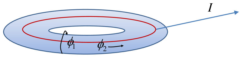
Figure 1: Geometry of action-angle-angle coordinates on cylinder torus with periodic orbit (red)

The dynamics of (5) evolves on a cylinder torus and consist of periodic orbits (refer to Fig. 1 for the schematic). In this paper, we are interested in time periodic volume preserving perturbations of degenerate action-angle-angle flows as given in (5) and the three dimensional maps that arise from it after taking appropriate Poincare section. We study the perturbation of the above discussed Hill spherical vortex flow for the case of large swirl in further detail in section IV.

Geometrical structures such as invariant manifolds play an important role in understanding the transport dynamics - specifically mixing and the lack thereof - in such maps. From numerical studies and perturbation method calculations, no invariant two-dimensional structure persists upon perturbation from an integrable action-angle-angle map with degenerate angle [19]. However the numerical studies carried out in [19] do not consider the class of perturbations for which the main result of this paper is proved and in fact corresponds to class of perturbations that is indicated in [20] as ones with possibility of having invariant tori. Dynamics related to transport in phase space for action-angle-angle maps with dynamically degenerate angle has been studied systematically in [20] where it is shown that for a large class of such maps, upon perturbation, most of the invariant surfaces are broken. The invariant surfaces break where resonance exists and at these locations in phase space, periodic orbits of specific types persist and dominate transport. This has been named Resonance-Induced Dispersion [19]. The result in this paper proves that, for a different class of perturbations, whose structure was also discussed in [20], two-dimensional invariant tori indeed exists for the perturbed action-angle-angle maps with degenerate angle satisfying intersection property - a condition that is implied by volume preservation. This proves the conjecture on such maps stated in [20].

The KAM type of result for the action-angle-angle maps is analogous to the degenerate Hamiltonian case treated by Arnold [3]. In proving this degenerate case of KAM, we are faced with two important problems. The first is due to unequal numbers of fast and slow variables. Because of this a drift term is introduced at each step of the coordinate transformations, we solve this problem by using proof techniques similar to the one which appears in [15]. The second problem is due to the degenerate nature of the one of the angles. We solve this problem by introducing an intermediate finite sequence of coordinate transformations. This finite sequence of coordinate transformations is different from the intermediate coordinate transformations which appear in Arnold’s proof [3] of degenerate KAM. The difference arises because of the difficulty with carrying out the Moser strategy of solution of the sequence of equations by backward substitution which in this case leads to $O(1)$ terms after an iteration step. Thus our proof is different in nature from the degenerate KAM proof which appears in [3].

The paper is organized as follows. In section II, we state the main theorem for the persistence of invariant tori in action-angle-angle maps with a degenerate angle. In section III, we give an outline of the proof. Simulation results for the Hill’s spherical vortex example are presented in section IV followed by conclusions in section V.

II Formulation of the theorem

Consider the following mapping

$$M=\left\{\begin{array}[]{ccl}x_{1}&=&x+f(z)+\epsilon{\cal X}(x,y,z)\\ y_{1}&=&y+\epsilon g_{0}(z)+\epsilon{\cal Y}(x,y,z)\;\;\;\;(x,y\;\;\;{\rm mod\;2\pi})\\ z_{1}&=&z+\epsilon{\cal Z}(x,y,z)\end{array}\right.$$ (6)

where ${\cal X}$,${\cal Y}$, and ${\cal Z}$ are real analytic functions of period $2\pi$ in $(x,y)$ with $\epsilon$ being a small positive number. The $f$ and $g_{0}$ are analytic functions of $z\in[a,b]=G$. To simplify the analysis we assume that $f(z)=z$ and $|g_{0}|\leq 1$. Since $\cal X,Y$ and, $\cal Z$ are real analytic functions, they can be extended to a complex domain:

$$D\;\;:|{\mathbf{I}m}\;{x}|<r\leq 1,\;\;\;\;\;|{\mathbf{I}m}\;{y}|<r\leq 1,\;\;\;\;\;z\in{\cal G},$$ (7)

where ${\cal G}$ is the complex neighborhood of the interval $[a,b]$. We now make following assumptions on the mapping (6).

Assumption 1

The functions $\cal Y$ and $Z$ are assumed to satisfy

$\int_{0}^{2\pi}{\cal Y}dx=\int_{0}^{2\pi}{\cal Z}dx=0$.

The condition $\int_{0}^{2\pi}{\cal Y}dx=0$ can be relaxed by requiring that the integral $\int_{0}^{2\pi}{\cal Y}dx$ be only a function of $z$ because any function of $z$ can always be absorbed in $g_{0}(z)$.

Assumption 2

Mapping (6) need not be measure preserving but we assume that the map satisfies the intersection property, i.e., any torus of the form:

$$z=\gamma(x,y)\;\;\;{\rm where}\;\;\;\gamma(x+2\pi,y)=\gamma(x,y)\;\;\&\;\;\;\gamma(x,y+2\pi)=\gamma(x,y)$$ (8)

intersect its image under the mapping.

Assumption 3

The function $g_{0}$ satisfies $g_{0}^{{}^{\prime\prime}}(z)\geq c_{1}>0$. $g_{0}^{{}^{\prime\prime}}>0$ is also referred to as second twist condition [15].

Now we state the main theorem for the persistence of invariant tori in the action-angle-angle map with one degenerate angle.

Theorem 4

Consider the mapping (6) satisfying assumptions 1, 2, and 3. There exists a positive number $\epsilon_{0}$ depending upon domain $D$, such that on $D$ and for all $\epsilon\in(0,\epsilon_{0})$, the mapping (6) admits a family of invariant tori of the form:

$$x=\xi+u(\xi,\zeta,\omega),\;\;\;\;\;y=\zeta+v(\xi,\zeta,\omega),\;\;\;\;\;z=w(\xi,\zeta,\omega),$$ (9)

where $u,v,w$ are real analytic functions of period $2\pi$ in the complex domain $|{\mathbf{I}m}\;x|<\frac{r}{2}$, $|{\mathbf{I}m}\;y|<\frac{r}{2}$ with $\omega\in S_{\omega}\subset G=[a,b]$, and $S_{\omega}$ is a Cantor set with positive Lebesgue measure. Moreover the mapping can be parameterized so that the induced mapping on the tori is given by

$$\xi_{1}=\xi+\omega,\;\;\;\;\;\zeta_{1}=\zeta+\epsilon g_{0}(\omega)+g^{*}(\omega,\epsilon),$$ (10)

where $g^{*}(\omega,\epsilon)$ is an analytic function that satisfies $g^{*}(\omega,0)=0$.

III Outline of the proof

The proof consists of applying coordinate transformations in three different steps. The first step of averaging coordinate transformation is applied to reduce the size of all the three perturbations to order $\epsilon^{2}$. The second step consists of applying a finite sequence of coordinate transformations to reduce the size of the action perturbation to order $\epsilon^{3}$. In the third and final step, we apply an infinite sequence of coordinate transformations similar to the one applied in proving the classical KAM theorem [2, 3, 5, 15], but with some modifications.

III-A First coordinate transformation

With $f(z)$ replaced with $z$ in (6), we denote the original mapping $M$ (Eq. 6) by $M_{0}$ and write it as follows:

$$M_{0}=\left\{\begin{array}[]{ccl}x_{1}&=&x+z+\epsilon{\cal X}(x,y,z)\\ y_{1}&=&y+\epsilon g_{0}(z)+\epsilon{\cal Y}(x,y,z)\;\;\;\;(x,y\;\;\;{\rm mod\;\;2\pi})\\ z_{1}&=&z+\epsilon{\cal Z}(x,y,z).\end{array}\right.$$ (11)

This map is defined in the complex domain $D$ (Eq. 7). Now we prove the main Lemma of the first coordinate transformation. This Lemma is similar to the averaging Lemma from [3].

Lemma 5

Consider a coordinate transformation $I_{\epsilon}$, defined in domain $D$, of the form:

$$I_{\epsilon}=\{\bar{x}=x+\epsilon h_{1}(x,y,z),\;\;\;\;\;\bar{y}=y+\epsilon h_{2}(x,y,z),\;\;\;\;\;\bar{z}=z+\epsilon h_{3}(x,y,z),$$

where $h_{1},h_{2}$ and $h_{3}$ are real analytic functions and periodic with period $2\pi$ in $x$ and $y$. Using this coordinate transformation, the mapping $M_{0}$ (Eq. 11), defined in the domain $D$, is transformed to the form $\bar{M}_{0}=I_{\epsilon}M_{0}I_{\epsilon}^{-1}$

$$\bar{M}_{0}=\left\{\begin{array}[]{ccl}\bar{x}_{1}&=&\bar{x}+\bar{z}+\bar{X}(\bar{x},\bar{y},\bar{z})\\ \bar{y}_{1}&=&\bar{y}+\epsilon g_{0}(\bar{z})+\bar{Y}(\bar{x},\bar{y},\bar{z})\;\;\;\;(x,y\;\;\;{\rm mod2\pi})\\ \bar{z}_{1}&=&\bar{z}+\bar{Z}(\bar{x},\bar{y},\bar{z}).\end{array}\right.$$

The mapping $\bar{M}_{0}$ is defined in a smaller domain:

$$\bar{D}:|{\mathbf{I}m}\;x|<r-\delta,\;\;\;\;|{\mathbf{I}m}\;y|<r-\delta,\;\;\;\;z\in{\cal G}^{{}^{\prime}},$$

where $\delta$ is a small positive number. The domain ${\cal G}^{{}^{\prime}}$ is the complex neighborhood of $G^{{}^{\prime}}$ and $G^{{}^{\prime}}$ is obtained from $G=[a,b]$ by removing finite number of resonance zones. In this reduced domain $G^{{}^{\prime}}$, $z$ satisfies following inequalities

$$|kz+2\pi n|\geq\bar{K}|k|^{-\bar{\mu}}\;\;\;(0<|k|\leq N),$$

where $\bar{K}$ is a positive constant, $N$ is a large integer, and $\bar{\mu}\geq 3$. We have the following estimates on the perturbations $\bar{X},\bar{Y},\bar{Z}$ in the domain $\bar{D}$

$|\bar{X}|+|\bar{Y}|+|\bar{Z}|<\epsilon^{2}=d_{0}$.

Proof:

: The difference equation (11) in the new coordinates can be written as follows:

$$\bar{x}_{1}=\bar{x}+\bar{z}+\epsilon{\cal X}^{1}+O(\epsilon^{2}),\;\;\;\bar{y}_{1}=\bar{y}+\epsilon g(\bar{z})+\epsilon{\cal Y}^{1}+O(\epsilon^{2}),\;\;\;\bar{z}_{1}=\bar{z}+\epsilon{\cal Z}^{1}+O(\epsilon^{2}).$$

The size of the perturbations in the new coordinate will be of the order $\epsilon^{2}$ if each of the following terms is of order $\epsilon$.

$${\cal X}^{1} := {\cal X}(x,y,z)+h_{1}(x+z,y,z)-h_{1}(x,y,z)-h_{3}(x,y,z)$$

$${\cal Y}^{1} := {\cal Y}(x,y,z)+h_{2}(x+z,y,z)-h_{2}(x,y,z)$$

$${\cal Z}^{1} := {\cal Z}(x,y,z)+h_{3}(x+z,y,z)-h_{3}(x,y,z)$$ (12)

Perturbations $\cal X,Y,$ and $\cal Z$ can be expressed in the Fourier series as

$${\cal X}=\sum_{k=-\infty}^{\infty}{\cal X}_{k}(y,z)e^{ikx},\;\;{\cal Y}=\sum_{k=-\infty}^{\infty}{\cal Y}_{k}(y,z)e^{ikx},\;\;{\cal Z}=\sum_{k=-\infty}^{\infty}{\cal Z}_{k}(y,z)e^{ikx}.$$

Now we represent each of the $h_{i}$ by the finite series $h_{i}=\sum_{|k|\leq N}h_{i_{k}}(y,z)e^{ikx}$, where $h_{i_{k}}$ satisfies following equality for $|k|\leq N$:

$$h_{1_{k}}=\frac{{\cal X}_{k}-h_{3_{k}}}{(1-e^{ikz})},\;\;\;h_{2_{k}}=\frac{{\cal Y}_{k}}{(1-e^{ikz})},\;\;\;h_{3_{k}}=\frac{{\cal Z}_{k}}{(1-e^{ikz})}.$$

To satisfy the above equation for bounded $h_{ik}$, we require $z$ to satisfy the following inequalities:

$$|kz+2\pi n|\geq\bar{K}|k|^{-\bar{\mu}}\;\;\;(0<|k|\leq N),$$

for some positive constant $\bar{K}$ and $\bar{\mu}\geq 3$. Since average value of $\cal Z$ and $\cal Y$ with respect to $x$ is equal to zero, $h_{3_{0}}$ and $h_{2_{0}}$ are free to take any value. We make $h_{3_{0}}={\cal X}_{0}$ so as to satisfy first equality of (12). With these choices of $h_{i}$ (12) reduces to

$${\cal X}^{1}=\sum_{|k|>N}{\cal X}_{k}e^{ikx},\;\;{\cal Y}^{1}=\sum_{|k|>N}{\cal Y}_{k}e^{ikx},\;\;{\cal Z}^{1}=\sum_{|k|>N}{\cal Z}_{k}e^{ikx}.$$

Each of these terms will be of order $\epsilon$, if $N$ is chosen sufficiently large to be of order greater than $\frac{1}{\delta}\ln{\frac{2}{(1-e^{-\delta})\epsilon}}$, (refer to [3], technical Lemmas on page 163). The $\delta$ is related to the new domain $\bar{D}$ as follows:

$$\bar{D}\;\;:|{\mathbf{I}m}\;{x}|<r-\delta,\;\;\;|{\mathbf{I}m}\;{y}|<r-\delta,\;\;\;z\in{\cal G}^{{}^{\prime}}.$$

This new complex domain ${\cal G}^{{}^{\prime}}$ of $z$ is a complex neighborhood of $G^{{}^{\prime}}$, where $G^{{}^{\prime}}$ is obtained from $G$ after removing the finite number of resonance intervals. The total measure of the resonance intervals has an upper bound of $(b-a)2\bar{K}$, so that the reduced domain is of order 1 for small value of $\bar{K}$ (refer to [3], technical Lemmas on page 163).

In this new domain following inequalities are satisfied

$$|kz+2\pi n|\geq\bar{K}|k|^{-\bar{\mu}}\;\;\;(0<|k|\leq N).$$

∎

After this first averaging coordinate transformation, we get following estimates on the perturbations

$$|\bar{X}|+|\bar{Y}|+|\bar{Z}|<\epsilon^{2}=d_{0}.$$

The action variable $z$ now belongs to the domain which is a function of $\epsilon$ i.e., $z\in G^{{}^{\prime}}(\epsilon)$ and the magnitude of the connected components of $G^{{}^{\prime}}$ is going to zero as $(\ln\frac{1}{\epsilon})^{-2}$.

At this point it seems that with some work is needed to deal with the $(\ln\frac{1}{\epsilon})^{-2}$ shrinkage of connected components of $G^{{}^{\prime}}$, we should be able to utilize results of [13] to conclude existence of a Diophantine invariant tori in the perturbed mapping. However, careful examination of the proof of the result in [13] reveals that the proof holds true only under the additional assumption that the perturbation $\bar{Z}=0$. The assumption of $\bar{Z}=0$ is clearly not satisfied in our case since $\cal Z$ is not assumed to be zero. In fact, the finite sequence of coordinate transformations discussed in the following section are precisely introduced to decrease the size of action perturbation $\bar{Z}$ relative to other perturbations, if not to make it zero.

III-B Second coordinate transformation

At this point we would like to continue with the standard infinite sequence of coordinate transformations as in Moser [5] but we are faced with the following problem. The aim is to reduce the size of all the three perturbations $\bar{X},\bar{Y}$ and $\bar{Z}$. Due to the degenerate nature of the angle $y$, the small denominator problem is exaggerated. The degenerate angle $y$ introduces a term of order $\frac{1}{\epsilon}$ in the estimates, which gives $O(1)$ estimates for the size of the coordinate transformation. This makes it impossible to continue with the infinite sequence of coordinate transformations. This problem can be solved by introducing an intermediate finite sequence of coordinate transformations. The aim of the finite sequence of coordinate transformations is to reduce the size of action perturbation $Z$ to order $\epsilon^{3}$ so that $\frac{1}{\epsilon}$ order term introduced by the degenerate angle can be compensated.

For notational convenience we remove the over-bar notation from the coordinates and the perturbations $\bar{X},\bar{Y}$ and $\bar{Z}$ and parameterize the map by $\omega$. The new map after the first coordinate transformation is denoted by $M_{0}(\omega)$. At this stage it is not really necessary to parameterize the mapping by $\omega$ however the importance of this parameterization will become clear later in the infinite sequence of coordinate transformations. We have,

$$M_{0}(\omega)=\left\{\begin{array}[]{ccl}x_{1}&=&x+\omega+z+X(x,y,z,\omega)\\ y_{1}&=&y+\epsilon g_{0}(z,\omega)+Y(x,y,z,\omega)\\ z_{1}&=&z+Z(x,y,z,\omega)\end{array}\right.$$

defined in the domain:

$$D_{0}(\omega):|{\mathbf{I}m}\;x|<\hat{r}_{0}<1,\;\;\;\;\;|{\mathbf{I}m}\;y|<\hat{r}_{0}<1,\;\;\;\;\;|z|<\hat{s}_{0},\;\;\;\;\omega\in G^{{}^{\prime}},$$

where $\hat{r}_{0},\hat{s}_{0}$ are positive numbers defined later and $|X|+|Y|+|Z|<d_{0}$ in $D_{0}(\omega)$. The mapping $M_{0}(\omega)$ is parameterized such that $g_{0}(z,\omega)=g_{0}(z+\omega),X(x,y,z,\omega)=X(x,y,z+\omega)$ and so on for $Y$ and $Z$. In the second coordinate transformation we treat this map as an action-angle map, where $x$ is the angle and $z$ is the action, and we consider $y$ as a parameter. Note that $\omega\in G^{{}^{\prime}}$, and the magnitude of the connected components of $G^{{}^{\prime}}$ is going to zero as $(\ln\frac{1}{\epsilon})^{-2}$. In order to account for the shrinking size of the connected components of the domain $G^{{}^{\prime}}$ with decreasing $\epsilon$, we require $\omega$ to satisfy infinitely many inequalities of the form:

$$|k\omega+2\pi n|\geq\epsilon^{\gamma_{1}}\hat{K}|k|^{-\hat{\mu}}\;\;\;(k,n=1,2,...),$$ (13)

where $\hat{K}$ is a positive constant, $\hat{\mu}\geq 3$, and $\gamma_{1}$ is a suitably chosen constant satisfying $0<\gamma_{1}<<1$. The introduction of $\epsilon^{\gamma_{1}}$ term in (13) ensures that while the size of the domain $G^{{}^{\prime}}$ goes to zero as $(\ln\frac{1}{\epsilon})^{-2}$ the reduction in the size of perturbation can be obtained in the neighborhood of the nonresonant value of action, the length of which tends to zero as power of $\epsilon$. Now we show that after applying finitely many coordinate transformations we can reduce the size of action perturbation $Z$ to order $d_{0}^{\frac{3}{2}}$. Let $T_{i}(\omega)$ denote these coordinate transformations. Let $M_{k}(\omega)=T_{k-1}^{-1}(\omega)M_{k-1}(\omega)T_{k-1}(\omega)$ be the mapping obtained after applying these coordinate transformations and defined in the domain $D_{k}(\omega)$. We will suppress the dependence on $\omega$ of the mapping $M$ and coordinate transformation $T$ at some places for notational convenience. We have following Lemma for the intermediate step of coordinate transformation.

Lemma 6

There exists a coordinate transformation $T(\omega)$ of the form:

$$T(\omega)=\{x=\varphi+\hat{U}(\varphi,\psi,\eta,\omega),\;\;\;\;y=\psi,\;\;\;\;z=\eta+\hat{W}(\varphi,\psi,\eta,\omega)$$ (14)

such that the mapping $M_{0}(\omega)$ (Eq. III-B) defined in the domain:

$${\cal A}_{0}(\omega):|{\mathbf{I}m}\;x|<\hat{r},\;\;\;\;|{\mathbf{I}m}\;y|<\hat{r},\;\;\;\;|z|<\hat{s},$$

with $|X|+|Y|+|Z|<d$, takes the form $M(\omega)=T^{-1}(\omega)M_{0}(\omega)T(\omega)$

$$M(\omega)=\left\{\begin{array}[]{ccl}\varphi_{1}&=&\varphi+\omega+\eta+\hat{X}(\varphi,\psi,\eta,\omega)\\ \psi_{1}&=&\psi+\epsilon g_{0}(\eta,\omega)+\hat{Y}(\varphi,\psi,\eta,\omega)\\ \eta_{1}&=&\eta+\hat{Z}(\varphi,\psi,\eta,\omega).\end{array}\right.$$ (15)

The mapping $M(\omega)$ is defined in the smaller domain ${\cal A}_{1}(\omega):|{\mathbf{I}m}\;\varphi|<\hat{\rho}$, $|{\mathbf{I}m}\;\psi|<\hat{\rho}$, $|\eta|<\hat{\sigma}$, with $0<\hat{\rho}<\hat{r}$, $0<\hat{\sigma}<\hat{s}$. Assume that

$$\hat{r}<1,\;\;0<3\hat{\sigma}<\hat{s}<\frac{\hat{r}-\hat{\rho}}{4},\;\;\;d<\frac{\hat{s}}{6},\;\;\;\hat{\vartheta}<\frac{\hat{\vartheta}_{2}}{\hat{s}}<\frac{1}{7},$$ (16)

$${\rm where}\;\;\;\hat{\vartheta}=\frac{a_{1}}{\hat{K}^{2}}(\hat{r}-\hat{\rho})^{-2\hat{\mu}-2}\frac{d}{\hat{s}}\epsilon^{-2\gamma_{1}}<\frac{1}{7},\;\;\;\hat{\vartheta_{2}}=\frac{a_{1}}{\hat{K}^{4}}(\hat{r}-\hat{\rho})^{-4\hat{\mu}-3}d\epsilon^{-4\gamma_{1}},\;\;\;$$

and $a_{1}$ is a positive constant independent of the domain and depends only upon $\hat{\mu}$. Using the above assumptions, we get following estimates for $\hat{U},\hat{W},\hat{X},\hat{Y}$, and $\hat{Z}$

$$|\hat{Y}| < d,\;\;\;\;|\hat{U}|+|\hat{W}|<\hat{\vartheta}\hat{s},$$

$$|\hat{X}|+|\hat{Z}| < a_{4}\Big{(}(\hat{r}-\hat{\rho})^{-2\hat{\mu}-3}\epsilon^{-2\gamma_{1}}d\hat{s}+(\hat{r}-\hat{\rho})^{-2\hat{\mu}-3}\epsilon^{-2\gamma_{1}}\frac{d^{2}}{\hat{s}}$$

$$+ (\hat{r}-\hat{\rho})^{-2\hat{\mu}-3}\epsilon^{1-2\gamma_{1}}d+(\frac{\hat{\sigma}}{\hat{s}})^{5}d\Big{)},$$

where $a_{4}$ is a positive constant independent of the domain.

The proof of this Lemma is similar to the Moser version of the KAM proof for action-angle maps [5] with the difference being that the angle variable $y$ in this proof is treated as a parameter. We refer the readers to [5] (Chapter 3; Section 32) for the proof. We now use the result of this Lemma to prove that at the end of the second coordinate transformation, the size of action perturbation $Z$ is of order $d_{0}^{\frac{3}{2}}$. To this end we apply the Lemma to the mapping $M_{0}(\omega)$ defined in the domain:

$$D_{0}(\omega):|{\mathbf{I}m}\;x|<\hat{r}_{0},|{\mathbf{I}m}\;y|<\hat{r}_{0},|z|<\hat{s}_{0},$$

where $D_{0}(\omega)$ correspond to the domain ${\cal A}_{0}(\omega)$ of the Lemma. By assumption, we have

$$|X|+|Y|+|Z|<d_{0}\;\;{\rm in}\;\;D_{0}(\omega).$$

Transforming the mapping $M_{0}(\omega)$ by the coordinate transformation $T_{0}(\omega)=T(\omega)$ provided by the Lemma, we obtain the mapping $M_{1}(\omega)=T_{0}^{-1}(\omega)M_{0}(\omega)T_{0}(\omega)$ defined in the domain:

$D_{1}(\omega):|{\mathbf{I}m}\;x|<\hat{r}_{1},\;|{\mathbf{I}m}\;y|<\hat{r}_{1},\;|z|<\hat{s}_{1}$,

where $D_{1}(\omega)$ correspond to the domain ${\cal A}_{1}(\omega)$ and $\hat{r}_{1},\hat{s}_{1}$ corresponds to the parameter $\hat{\rho},\hat{\sigma}$ of the Lemma. We define the following sequences

$$\hat{r}_{n}=\frac{\hat{r}_{0}}{2}(1+\frac{1}{2^{n}}),\;\;\hat{s}_{n}=d_{n}^{\frac{11}{50}},\hat{s}_{0}=\hat{s},\;\;d_{n+1}=\hat{r}_{0}^{-\hat{\chi}}\hat{c}_{7}^{n+1}d_{n}^{\frac{6}{5}}\epsilon^{-2\gamma_{1}},\;\;\hat{\chi}=2\hat{\mu}+3$$

$$\hat{r}_{0}=r-\delta,\;\;\;\hat{c}_{7}>3,\;\;d_{0}<\hat{c}_{7}^{-20}\hat{r}_{0}^{7\hat{\chi}}\epsilon^{14\gamma_{1}}.$$

For the above sequences to be well defined we require that $\gamma_{1}<\frac{1}{5}$. We need to check whether these sequences satisfies the inequality (16). Towards this we have,

$$(\frac{\hat{s}_{n+1}}{\hat{s}_{n}})^{\frac{50}{11}}=\frac{d_{n+1}}{d_{n}}=\hat{c}_{7}^{n+1}d_{n}^{\frac{1}{5}}=e_{n}^{\frac{1}{5}}\hat{c}_{7}^{-5}\hat{r}_{0}^{\hat{\chi}},$$

where $e_{n}=\hat{r}_{0}^{-5\hat{\chi}}\hat{c}_{7}^{5(n+6)}\epsilon^{10\gamma_{1}}d_{n}$ and $e_{n+1}=e_{n}^{\frac{6}{5}}$. Since $d_{0}<\hat{c}_{7}^{-20}\hat{r}_{0}^{7\hat{\chi}}\epsilon^{14\gamma_{1}}$, we have $e_{0}<1$ and

$$\frac{s_{n+1}}{s_{n}}<\hat{c}_{7}^{\frac{-11}{10}}<\frac{1}{3},\;\;\;\;{\rm since}\;\;\hat{c}_{7}>3.$$

The inequality $\hat{s}_{n}=d_{n}^{\frac{11}{50}}<\frac{\hat{r}_{n}-\hat{r}_{n+1}}{4},d_{n}<\frac{\hat{s}_{n}}{6},\;\;{\rm and}\;\;\hat{\vartheta}<\frac{1}{7}$ can be satisfied by taking $d_{0}$ sufficiently small and using the fact that

$$\hat{r}-\hat{\rho}=\hat{r}_{n}-\hat{r}_{n+1}=\hat{r}_{0}2^{-n-2},\;\;\;\hat{s}_{n}=d_{n}^{\frac{11}{50}}.$$

Using $d_{n+1}=\hat{r}_{0}^{-\hat{\chi}}\hat{c}_{7}^{n+1}d_{n}^{\beta}\epsilon^{-2\gamma_{1}}$ with $\beta=\frac{6}{5}$, we have

$$d_{n+1}=\hat{r}_{0}^{-\hat{\chi}(\sum_{k=1}^{n}\beta^{k})}\hat{c}_{7}^{(n+1+n\beta+(n-1)\beta^{2}+...+\beta^{n})}\epsilon^{-2\gamma_{1}(\sum_{k=1}^{n}\beta^{k})}d_{0}^{\beta^{n+1}}.$$

We want that after finitely many coordinate transformations $d_{n+1}<d_{0}^{\frac{3}{2}}$. Using the fact that $\epsilon=d_{0}^{\frac{1}{2}}$ and $d_{0}<\hat{c}_{7}^{-20}\hat{r}_{0}^{7\hat{\chi}}\epsilon^{14\gamma_{1}}$, it follows for $n=5$ that $d_{6}<d_{0}^{\frac{3}{2}}$ and we get,

$$|\hat{X}_{6}|+|\hat{Z_{6}}|<a_{4}\Big{(}2^{7(2\hat{\mu}+3)}\hat{c}_{7}^{-6}d_{5}^{\frac{1}{50}}+2^{7(2\hat{\mu}+3)}\hat{c}_{7}^{-6}d_{5}^{\frac{29}{50}}+\hat{r}_{0}^{\hat{\chi}}2^{7(2\hat{\mu}+3)}\hat{c}_{7}^{-10}+(\frac{d_{6}}{d_{5}})^{\frac{1}{10}}\Big{)}d_{6}.$$

The coefficient multiplying $d_{6}$ can be made less than one by choosing $\hat{c}_{7}$ sufficiently large, $\gamma_{1}$ sufficiently small, and noticing that $\frac{d_{6}}{d_{5}}<1$ to give us

$$|\hat{X}_{6}|+|\hat{Z_{6}}|<d_{6}<d_{0}^{\frac{3}{2}}.$$

III-C Infinite sequence of coordinate transformation

At this stage of infinite sequence of coordinate transformations, our aim is to decrease the size of all the three perturbations simultaneously. In both the KAM proof for Moser twist map [5], and the action-angle-angle maps [15], the size of all the perturbations decreases simultaneously with the same estimates on the perturbations at each step of the infinite sequence of coordinate transformations. In our proof, due to the degenerate nature of the angle $y$, we require that the size of action perturbation $Z$ is always $d^{\frac{1}{2}}$ order smaller than the angle perturbations. This requires us to estimate the size of action perturbation $Z$ separately from the size of the angles perturbations $X$ and $Y$.

Now we have a problem which is different from the Moser version of the KAM proof for the twist maps, but similar to the one faced in proving the KAM theorem for action-angle-angle maps. The problem is due to unequal numbers of action and angle variables. Due to this problem, it is not possible to predict which tori will survive the perturbation and hence at this stage it becomes necessary to parameterize the mapping by $\omega$.

We denote the mapping obtained after the second coordinate transformation $M_{6}(\omega)$ by ${\cal M}_{0}(\omega)$. We are using the same notation for the perturbation $X,Y$, and $Z$ as at the beginning of the second coordinate transformation i.e., we define $X:=\hat{X}_{6},Y:=\hat{Y}_{6},Z:=\hat{Z}_{6}$ and again the parametrization on $X,Y,Z$ and $g_{0}$ are chosen such that $X(x,y,z,\omega)=X(x,y,z+\omega)$ and $g_{0}(z,\omega)=g_{0}(z+\omega)$ and so on for $Y$ and $Z$. So we have

$${\cal M}_{0}(\omega)=\left\{\begin{array}[]{ccl}x_{1}&=&x+\omega+z+X(x,y,z,\omega)\\ y_{1}&=&y+\epsilon g_{0}(z,\omega)+Y(x,y,z,\omega)\\ z_{1}&=&z+Z(x,y,z,\omega),\end{array}\right.$$ (17)

with $|X|<d_{0}^{\frac{3}{2}}<d_{0}$, $|Y|<d_{0}$, and $|Z|<d_{0}^{\frac{3}{2}}$ defined in domain ${\cal D}_{0}(\omega):|{\mathbf{I}m}\;x|<r_{0}\leq\hat{r}_{6},\;\;|{\mathbf{I}m}\;y|<r_{0}\leq\hat{r}_{6},\;\;|z|<s_{0}\leq\hat{s}_{6}$. To account for the shrinking size of the connected components of domain $G^{{}^{\prime}}(\epsilon)\ni\omega$ with decreasing $\epsilon$, in this step of coordinate transformation we require $(\omega,\epsilon g_{0}(\omega))$ to satisfy infinitely many inequalities of the form:

$$|k_{1}\omega+\epsilon k_{2}g_{0}(0,\omega)+2\pi n|\geq\left\{\begin{array}[]{ccl}\epsilon^{\gamma_{2}}K|k|^{-\mu}&{\rm if}&k_{1}\neq 0\\ \epsilon^{1+\gamma_{2}}K|k|^{-\mu}&{\rm if}&k\neq 0\end{array}\right.\forall(k_{1},k_{2},n)\in{\mathbf{Z}}^{3}\setminus\{0\},$$ (20)

where $|k|=|k_{1}|+|k_{2}|$, $K$ some positive constant, $\mu\geq 5$ and $\gamma_{2}$ is sufficiently small positive constant i.e., $0<\gamma_{2}<<1$. Now we use an infinite sequence of coordinate transformations similar to the one used in [5] but with some modification. We have following induction Lemma for the third and final step of coordinate transformation.

Lemma 7

There exists a coordinate transformation ${\cal U}(\omega)$ of the form:

$${\cal U}(\omega)=\{x=\varphi+U(\varphi,\psi,\eta,\omega),\;\;\;\;\;y=\psi+V(\varphi,\psi,\eta,\omega),\;\;\;\;\;z=\eta+W(\varphi,\psi,\eta,\omega)\;\;\;\;\;$$

such that the mapping ${\cal M}_{0}(\omega)$ (Eq. 17), defined in the domain:

$${\cal B}_{0}(\omega):|{\mathbf{I}m}\;x|<r,\;\;\;\;\;|{\mathbf{I}m}\;y|<r,\;\;\;\;\;|z|<s,$$

with $|X|+|Y|<d$ and $|Z|<d^{\frac{3}{2}}$ takes the form ${\cal M}(\omega)={\cal U}^{-1}(\omega){\cal M}_{0}(\omega){\cal U}(\omega)$. The mapping ${\cal M}(\omega)$

$${\cal M}(\omega)=\left\{\begin{array}[]{lll}\varphi_{1}=\varphi+\omega+\eta+\Phi(\varphi,\psi,\eta,\omega)\\ \psi_{1}=\psi+\epsilon g_{0}(\eta,\omega)+g_{1}(\eta,\omega)+\Psi(\varphi,\psi,\eta,\omega)\\ \eta_{1}=\eta+H(\varphi,\psi,\eta,\omega)\end{array}\right.$$

is defined in the following smaller domain:

$${\cal B}_{1}(\omega):|{\mathbf{I}m}\;\varphi|<\rho\;\;|{\mathbf{I}m}\;\psi|<\rho\;\;|\eta|<\sigma,$$

with $0<\rho<r,0<\sigma<s$. Now assume that

$$0<r\leq\hat{r}_{6},\;\;\;0<3\sigma<s<d^{\frac{1}{2}}(r-\rho),\;\;d<\frac{s}{2},\;\;\;\vartheta d^{\frac{1}{2}}<\frac{\vartheta_{2}d^{\frac{1}{2}}}{s}<\frac{1}{8},$$ (21)

$${\rm where}\;\;\vartheta=\frac{b_{1}}{K^{2}}(r-\rho)^{-2\mu-4}\epsilon^{-2\gamma_{2}}\frac{d^{\frac{1}{2}}}{s},\;\;\;\vartheta_{2}=\frac{b_{1}}{K^{4}}(r-\rho)^{-4\mu-4}\epsilon^{-2\gamma_{2}}d^{\frac{1}{2}}$$

and $b_{1}$ is a positive constant independent of the domain and depends only on $\mu$. Under the above assumptions, it follows that ${\cal M}(\omega)$ is well defined in ${\cal B}_{1}(\omega)$ and there are following estimates:

$$|U|+|V|<\frac{b_{1}}{K^{2}}(r-\rho)^{-2\mu-4}\epsilon^{-2\gamma_{2}}d^{\frac{1}{2}},\;\;\;|W|<\frac{b_{1}}{K}(r-\rho)^{-\mu-2}\epsilon^{-2\gamma_{2}}\frac{d^{\frac{3}{2}}}{\epsilon}$$

$$|\Phi|+|\Psi| < b_{6}\Big{(}\frac{(r-\rho)^{-2\mu-5}}{K^{2}}\epsilon^{-2\gamma_{2}}d^{\frac{1}{2}}s+\frac{(r-\rho)^{-2\mu-4}}{K^{2}}\epsilon^{-2\gamma_{2}}\frac{d^{\frac{1}{2}}}{s}|H|$$ (22)

$$+ \frac{(r-\rho)^{-2\mu-4}}{K^{2}}\epsilon^{-2\gamma_{2}}\frac{d^{2}}{s}+\frac{(r-\rho)^{-4\mu-8}}{K^{4}}\epsilon^{-4\gamma_{2}}\frac{d^{\frac{5}{2}}}{s^{2}}\Big{)}$$

$$|H| < b_{5}\Big{(}\frac{(r-\rho)^{-2\mu-5}}{K^{2}}\epsilon^{-2\gamma_{2}}ds+\frac{(r-\rho)^{-4\mu-8}}{K^{4}}\epsilon^{-4\gamma_{2}}\frac{d^{\frac{5}{2}}}{s}$$

$$+ \frac{(r-\rho)^{-6\mu-13}}{K^{6}}\epsilon^{-6\gamma_{2}}\frac{d^{\frac{7}{2}}}{s^{2}}+\frac{(r-\rho)^{-2\mu-4}}{K^{2}}\epsilon^{-2\gamma_{2}}\frac{d^{5/2}}{s}+(\frac{\sigma}{s})^{3}d^{\frac{3}{2}}\Big{)}$$

where $g_{1}(0,\omega)=-\epsilon g_{0\eta}(0,\omega)\tilde{X}(0,\omega)+\tilde{Y}(0,\omega)$, $\tilde{X}$ and $\tilde{Y}$ are average value of $X$ and $Y$ respectively and $b_{5},b_{6}$ are positive constants independent of the domain. The functions $g_{0}(0,\omega)$ and $g_{1}(0,\omega)$ satisfy the following new Diophantine conditions:

$$|k_{1}\omega+k_{2}(\epsilon g_{0}(0,\omega)+g_{1}(0,\omega))+2\pi n|\geq\left\{\begin{array}[]{ccl}\epsilon^{\gamma_{2}}\frac{K}{2}|k|^{-\mu}&{\rm if}&k_{1}\neq 0\\ \epsilon^{1+\gamma_{2}}\frac{K}{2}|k|^{-\mu}&{\rm if}&k\neq 0\end{array}\right.\forall(k_{1},k_{2},n)\in{\mathbf{Z}}^{3}\setminus\{0\}$$

Proof of this Lemma follows along the similar lines for the Moser version of the KAM proof for the action-angle map [5] (Chapter 3; Section 32). Due to unequal numbers of action and angle variables we have a problem which is different from the KAM proof for the twist map. The term $g_{1}(\eta,\omega)$ in the mapping ${\cal M}(\omega)$ of the Lemma gives rise to the shift in frequency of the degenerate angle. In general at the $(n+1)$ step of the coordinate transformation there is a frequency drift from $(\omega,\epsilon g_{0}(0,\omega)+\sum_{j=1}^{n}g_{j}(0,\omega))$ to $(\omega,\epsilon g_{0}(0,\omega)+\sum_{j=1}^{n+1}g_{j}(0,\omega))$ similar to the case in [15]. In order to compensate for this frequency drift we need to broaden the set of admissible values of $\omega$. This can be achieved by allowing the constant $K$ in inequalities (20) to decrease at each step of the coordinate transformation. However decreasing the size of $K$ will lead to increase in the size of estimates for the perturbations and hence the scheme to make the mapping closer to the double twist mapping might be a failure. We show that this is not always the case and there exists a nonempty set $S(\omega)\subset G$ on which corresponding $K$ decrease at most like power of $K_{0}$ $(K_{n}=\frac{K_{0}}{2^{n}})$ so that the size of the perturbations decreases exponentially. To prove this we employ the strategy similar to that in [15] with the difference that while the strategy in [15] is developed for action-angle-angle map with no degeneracy in angle, we extend it to the case of degenerate angle. More specifically there are following differences between our proof and proof technique developed in [15]; 1) The averaging transformation is not needed in [15]; 2) The intermediate sequence of transformations is not needed in [15]; 3) The “Cantor set” calculations are substantially modified; 4) Whitney theory is used directly instead of doing it from scratch. Before explaining this strategy, we prove the following Lemma similar to the one in [15] except for the fact that the estimates in this Lemma are derived for the case of degenerate angle.

Lemma 8

Let $\epsilon>0$ be fixed and assume $\epsilon g_{0}(z)\in C^{2},g_{0}^{{}^{\prime\prime}}(z)\geq c_{1}>0$. Then the set $S(\omega)$, where

$$S(\omega)=\{\omega\in G^{{}^{\prime}}:|k\cdot\Omega+2\pi n|\geq\epsilon^{1+\gamma_{2}}K|k|^{-\mu},(\mu\geq 5),(k,n)\in{\mathbf{Z}}^{3}\setminus\{(0,0,0)\}\}$$

is a Cantor set with the Lebesgue measure $\mu_{l}(S(\omega))>\mu_{l}(G^{{}^{\prime}})-c_{3}\left(\frac{\epsilon^{\gamma_{2}}K}{c_{1}}\right)^{\frac{1}{2}}$ where, $(k\cdot\Omega)=k_{1}\omega+\epsilon k_{2}g_{0}(0,\omega)$, $c_{3}$ is a positive constant, and $\mu_{l}$ is the Lebesgue measure.

Proof:

For a fixed $(k_{1},k_{2},n)\in{\mathbf{Z}}^{3}$, consider the lines

$$l_{1}:\;\;k_{1}\omega_{1}+\epsilon k_{2}\omega_{2}+2\pi n=0,\;\;\;l_{2}:\;\;k_{1}\omega_{1}+\epsilon k_{2}\omega_{2}+2\pi n-\epsilon^{1+\gamma_{2}}K|k|^{-\mu}=0$$

$$l_{3}:\;\;k_{1}\omega_{1}+\epsilon k_{2}\omega_{2}+2\pi n+\epsilon^{1+\gamma_{2}}K|k|^{-\mu}=0.$$

The minimum distance between the lines $l_{1},l_{2}$ or $l_{1},l_{3}$ in the $(\omega_{1},\epsilon\omega_{2})$ plane is $\epsilon^{1+\gamma_{2}}K|k|^{-\mu}(k_{1}^{2}+k_{2}^{2})^{-\frac{1}{2}}$. Consider the points $(\omega_{1},\epsilon\omega_{2})$ in the set

$$\Omega_{1}=\{(\omega_{1},\epsilon\omega_{2})\in{\mathbf{R}}^{2}:d((\omega_{1},\epsilon\omega_{2}),l_{1})\geq\delta\},\\ \delta=\epsilon^{1+\gamma_{2}}K|k|^{-\mu}(k_{1}^{2}+k_{2}^{2})^{-\frac{1}{2}}.$$

The points in $\Omega_{1}$ set will satisfy the inequality (20) for a fixed $(k_{1},k_{2},n,K)$, where $d(\#,l)$ means the distance to the line $l$. Let $\Omega_{2}={\mathbf{R}}^{2}\setminus\Omega_{1}$, $\Gamma=$ graph $\epsilon g_{0}$, and $T_{1}$ the projection over first component. The length of $T_{1}|(\Gamma\cap{\Omega_{2}})$ is less than $4(\frac{\delta}{\epsilon c_{1}})^{\frac{1}{2}}$. For a fixed $k\in{\mathbf{Z}}^{2}$, if $(\omega_{1},\epsilon\omega_{2})$ is restricted in the domain $R_{\omega}$:

$$0\leq\min(\omega_{1},\epsilon\omega_{2})<\max(\omega_{1},\epsilon\omega_{2})\leq a_{8},$$

then the set $\Omega_{2}\cup R_{\omega}$ is non empty only if $|n|<\frac{a_{8}|k|}{2\pi}$. So the Lebesgue measure of the set $S(\omega)$ is

$$\mu_{l}(S(\omega))>\mu_{l}(G^{{}^{\prime}})-\frac{4a_{8}}{2\pi}\left(\frac{\epsilon^{\gamma_{2}}K}{c_{1}}\right)^{\frac{1}{2}}\sum_{k\in{\mathbf{Z}}^{2}}|k|^{\frac{-\mu}{2}+1}(k_{1}^{2}+k_{2}^{2})^{-\frac{1}{4}},$$

which is positive if $\mu\geq 5$ and $K$ is sufficiently small. Now

$$\frac{4a_{8}}{2\pi}\sum_{k\in\mathbf{Z}^{2}}|k|^{\frac{-\mu}{2}+1}(k_{1}^{2}+k_{2}^{2})^{-\frac{1}{4}}<\frac{4a_{8}}{2\pi}\sum_{k\in\mathbf{Z}^{2}}|k|^{\frac{-\mu}{2}+1-\frac{1}{4}}=:c_{3}$$

and the sum converge because $\mu\geq 5$ and $\mu_{l}(S(\omega))>\mu_{l}(G^{{}^{\prime}})-c_{3}(\frac{\epsilon^{\gamma_{2}}K}{c_{1}})^{\frac{1}{2}}$ ∎

We now introduce a sequence of coordinate transformation ${\cal U}_{n}(\omega)$ on a nonempty set $\tilde{S}_{n}\subset G^{\prime}$:

$${\cal M}_{n+1}(\omega)={\cal U}^{-1}_{n}(\omega){\cal M}_{n}(\omega){\cal U}_{n}(\omega),\;\;{\rm with}\;\;\tilde{S}_{n}(\omega)\subset\tilde{S}_{n-1}(\omega).$$

By Lemma 8, there exists a Cantor set $S_{0}(\omega)=\tilde{S}_{0}(\omega)$ given by

$$S_{0}(\omega)=\{\omega\in G^{{}^{\prime}}|(\omega,\epsilon g_{0}(0,\omega)){\rm\;satisfies\;(\ref{d1})\;with\;}K_{0}{\rm\;replacing\;}K\}.$$

The Lebesgue measure of the set $S_{0}(\omega)$ is $\mu_{l}(S_{0}(\omega))>\mu_{l}(G^{{}^{\prime}})-c_{3}\left(\frac{\epsilon^{\gamma_{2}}K_{0}}{c_{1}}\right)^{\frac{1}{2}},$where $\mu_{l}$ is the Lebesgue measure. Let $\tilde{S}_{1}(\omega)=\bigcap_{j=0}^{1}S_{j}(\omega)$, where

$$S_{1}(\omega)=\{\omega\in G^{{}^{\prime}}|(\omega,\epsilon g_{0}(0,\omega)+g_{1}(0,\omega)){\rm\;satisfies}\;(\ref{d1})\;{\rm with}\;\frac{K_{0}}{2}\;{\rm replacing}\;K\}.$$

In order to derive the Lebesgue measure of the set $S_{1}(\omega)$ we need $g_{1}(0,\omega)$ to be defined on the entire domain $G$. However, $g_{1}$ is only defined on the set $\tilde{S}_{0}(\omega)$. This problem can be solved using the Whitney extension theorem [21]. By using the Whitney extension theorem, we can extend the perturbations $X,Y,Z$ and subsequent perturbations $X_{j},Y_{j},Z_{j}$ coming from infinite sequence of coordinate transformation to the entire domain $G$ w.r.t. variable $\omega$. The proof for the extension follows along the lines of proof outlined in [11, 22]. Since $X,Y$, and $Z$ are extended to the domain $G$, the function $g_{1}$ is well defined for all values of $\omega\in G$ because

$$g_{1}(0,\omega)=-\epsilon g_{0\eta}(0,\omega)\tilde{X}(0,\omega)+\tilde{Y}(0,\omega),$$

where $\tilde{X}$ and $\tilde{Y}$ are the average values of $X$ and $Y$ respectively. We will use the same notation for the functions and its extension to the domain $G$ w.r.t. variable $\omega$ with the following estimate

$$\parallel X\parallel_{2,1,G}+\parallel Y\parallel_{2,1,G}<c_{w}d\;\;\;i=0,1,2,$$

where $c_{w}$ is the Whitney constant and is independent of the domain. The notation $\parallel\cdot\parallel_{2,1,G}$ is used as a measure for the norm of the function and the second derivative of the function w.r.t. variable $\omega$ in the domain $G$ (For more details on the norm refer to [22]). Differentiating $g_{1}(0,\omega)$ twice w.r.t. $\omega$ we get,

$$\left|\frac{d^{2}}{d\omega^{2}}g_{1}(0,\omega)\right|<5\sup(\epsilon g_{0\eta},\epsilon g_{0\eta\omega},\epsilon g_{0\eta\omega^{2}},1)c_{w}d<\epsilon\beta_{1}.$$

Hence

$$\frac{d^{2}}{d\omega^{2}}(\epsilon g_{0}+g_{1})>\epsilon(c_{1}-\beta_{1}),\;\;\;{\rm and}\;\;\;\mu_{l}(S_{1}(\omega))>\mu_{l}(G^{{}^{\prime}})-c_{3}\left(\frac{K_{0}\epsilon^{\gamma_{2}}}{2(c_{1}-\beta_{1})}\right)^{\frac{1}{2}}.$$

The measure of the set $S_{1}(\omega)$ is obtained from Lemma 8 by applying the results to $k\cdot\Omega=k_{1}\omega+k_{2}(\epsilon g_{0}+g_{1})$. Now $\tilde{S}_{1}(\omega)=S_{0}(\omega)\bigcap S_{1}(\omega)$ and

$$\mu_{l}(\tilde{S}_{1}(\omega))>\mu_{l}(G^{{}^{\prime}})-c_{3}\left(\frac{K_{0}\epsilon^{\gamma_{2}}}{c_{1}}\right)^{\frac{1}{2}}\left(1+\left(\frac{c_{1}}{2(c_{1}-\beta_{1})}\right)^{\frac{1}{2}}\right).$$

For $K_{0}$ and $\beta_{1}$ sufficiently small $\mu_{l}(\tilde{S}_{1}(\omega))$ is positive. We obtain the following expression for $g_{j+1}$ by induction on $g_{1}$ and its derivation is similar to that of $g_{1}$

$$g_{j+1}(0,\omega)=-\left(\epsilon g_{0\eta}(0,\omega)+\sum_{l=1}^{j}g_{l\eta}(0,\omega)\right)\tilde{X}_{j}(0,\omega)+\tilde{Y}_{j}(0,\omega),$$

where $X_{j}$ and $Y_{j}$ are extended to interval $G$ by using Whitney’s extension with the following estimates

$$\parallel X_{j}\parallel_{2,1,G}+\parallel Y_{j}\parallel_{2,1,G}<c_{w}d_{j}.$$

Assume that there exists a positive constant $c_{5}$ such that

$$\sup\left|\frac{d^{v}}{d\omega^{v}}(\epsilon g_{0\eta}(0,\omega)+\sum_{l=1}^{j}g_{l\eta}(0,\omega))\right|<c_{5}\;\;\;\;\;{v}=0,1,2.$$ (24)

The existence of such a positive constant $c_{5}$ can be proved as follows:

$$|\epsilon g_{0\eta}|\leq 1\;\;\;{\rm for}\;\;\eta\in G,\;\;{\rm and}\;\;|\epsilon g_{0\eta\omega^{2}}|\leq 1$$

$$|g_{1}|=|\epsilon g_{0\eta}\tilde{X}_{0}|+|\tilde{Y}_{0}|\leq 2d_{0},\;\;\;|g_{1\eta}|\leq\frac{2d_{0}}{s_{0}}\;\;\;{\rm for}\;\;|\eta|<s_{0},\;\;{\rm and}\;\;|g_{1\eta\omega^{2}}|\leq c_{w}\frac{2d_{0}}{s_{0}}$$

$$|g_{j+1}|\leq 2d_{j}\Pi_{i=1}^{j-1}(1+\frac{d_{i}}{s_{i}}),\;\;\;|g_{j+1,\eta}|\leq\frac{2d_{j}}{s_{j}}\Pi_{i=1}^{j-1}(1+\frac{d_{i}}{s_{i}})\;\;{\rm for}\;\;|\eta|<s_{j}\;\;{\rm and}\;\;$$

$$|g_{j+1,\eta\omega^{2}}|\leq\frac{c_{w}2d_{j}}{s_{j}}\Pi_{i=1}^{j-1}(1+\frac{d_{i}}{s_{i}}),$$

so by choosing $d_{0}$ sufficiently small it is possible to find the constant $c_{5}$ such that (24) is true. Now setting $c_{6}=5\max(c_{5},1)$ we get

$$\left|\frac{d^{2}}{d\omega^{2}}g_{j+1}(0,\omega)\right|<c_{6}c_{w}d_{j}=\epsilon\beta_{j+1},\;\;\;\;\sum_{l=1}^{j+1}\beta_{l}=\frac{c_{6}c_{w}}{\epsilon}\sum_{l=1}^{j+1}d_{l-1}$$

and this can be made less than $\frac{c_{1}}{2}$, if we choose $d_{0}$ sufficiently small. So we have $\sum_{l=1}^{j+1}\beta_{l}<\frac{c_{1}}{2}$ and then following inequality holds

$$\frac{d^{2}}{d\omega^{2}}(\epsilon g_{0\eta}(0,\omega)+\sum_{l=1}^{j+1}g_{l\eta}(0,\omega))>\epsilon c_{1}-\epsilon\sum_{l=1}^{j+1}\beta_{l}>\epsilon\frac{c_{1}}{2}.$$

By defining $\tilde{S}_{j+1}(\omega)=\bigcap_{l=0}^{j+1}S_{l}(\omega)$, where

$$S_{j+1}(\omega)=\{\omega\in G^{{}^{\prime}}|(\omega,\epsilon g_{0}(0,\omega)+\sum_{l=1}^{j+1}g_{l}(0,\omega))\;\;{\rm satisfies\;(\ref{d1})\;with}\;\;K_{j+1}=K_{0}/2^{j+1}\;{\rm in\;place\;of}\;K\},$$

we obtain,

$$\mu_{l}(S_{j+1}(\omega))>\mu_{l}(G^{{}^{\prime}})-c_{3}\left(\frac{K_{0}\epsilon^{\gamma_{2}}}{(c_{1}-\sum_{l=1}^{j+1}\beta_{l})2^{j+1}}\right)^{\frac{1}{2}}$$

$$\mu_{l}(\tilde{S}_{j+1}(\omega)) > \mu_{l}(G^{{}^{\prime}})-c_{3}\left(\frac{K_{0}\epsilon^{\gamma_{2}}}{c_{1}}\right)^{\frac{1}{2}}\sum_{l=1}^{j+1}2^{-l/2}\left(\frac{c_{1}}{c_{1}-\sum_{n=1}^{l}\beta_{n}}\right)$$

$$> \mu_{l}(G^{{}^{\prime}})-c_{3}\left(\frac{K_{0}\epsilon^{\gamma_{2}}}{c_{1}}\right)^{\frac{1}{2}}\sum_{l=0}^{j+1}2^{-l/2+1}.$$

The measure of set $\tilde{S}_{j+1}$ (i.e., $\mu_{l}(\tilde{S}_{j+1}(\omega))$) is positive if $K_{0}$ is sufficiently small. The total drift in the degenerate angle at the $j^{th}$ step of iteration is given by $\epsilon g_{0}(0,\omega)+\sum_{k=1}^{j}g_{j}(0,\omega)$ and in the limit as $j\to\infty$ we get $\epsilon g_{0}(0,\omega)+g^{*}(\omega,\epsilon)$, where $g^{*}(\omega,\epsilon):=\sum_{j=1}^{\infty}g_{j}(0,\omega)$.

Now we define a sequence similar to the one in [5]. Let $r_{n},r_{n+1},s_{n},s_{n+1},d_{n},\frac{K_{0}}{2^{n}}$ correspond to parameter $r,\rho,s,\sigma,d_{0},K$ respectively. Setting

$$r_{n}=\frac{r_{0}}{2}(1+\frac{1}{2^{n}}),\;\;\;K_{n}=\frac{K}{2^{n}},\;\;\;s_{n}=d_{n}^{\frac{11}{16}},\;\;\;s_{0}=\hat{s}_{6},\;\;\;d_{n+1}=r_{0}^{-\chi}c_{7}^{n+1}\epsilon^{-6\gamma_{2}}d_{n}^{\frac{9}{8}}$$

where $c_{7}>2$, $\chi=2\mu+5$ are suitable constants, $r_{n}$ converges to $\frac{r_{0}}{2}$, and $d_{n}$ converges to zero provided $d_{0}$ is chosen sufficiently small. The sequence $e_{n}=r_{0}^{-8\chi}c_{7}^{8(n+9)}\epsilon^{-48\gamma_{2}}d_{n}$ satisfies $e_{n+1}=e_{n}^{\frac{9}{8}}$ and hence converges to zero if we take $0<d_{0}^{1-24\gamma_{2}}<r_{0}^{8\chi}c_{7}^{-72}$. The inequality $3\sigma<s$ follows from

$(\frac{s_{n+1}}{s_{n}})^{\frac{16}{11}}=\frac{d_{n+1}}{d_{n}}=r_{0}^{-\chi}c_{7}^{n+1}d_{n}^{\frac{1}{8}}=e_{n}^{\frac{1}{8}}c_{7}^{-8}<\frac{1}{c_{7}^{8}}$, $\;\;\frac{s_{n+1}}{s_{n}}<\frac{1}{c_{7}^{5.5}}<\frac{1}{3}$, and $r_{n}-r_{n+1}=r_{0}2^{-n-2}$.

Now we will use induction Lemma to show that $|H_{n+1}|<d_{n+1}^{\frac{3}{2}}$ and $|\Phi_{n+1}|+|\Psi_{n+1}|<d_{n+1}$. By induction on second inequality of (22) and the fact that $s_{n}=d_{n}^{\frac{11}{16}}$ we have

$$|H_{j+1}| < b_{5}\Big{(}\frac{r_{0}^{\chi/2}2^{\chi(j+2)+2j}}{K_{0}^{2}}c_{7}^{-\frac{3}{2}(j+1)}\epsilon^{7\gamma_{2}}+\frac{r_{0}^{2-\frac{\chi}{2}}2^{2(\chi-1)(j+2)+4j}}{K_{0}^{4}}c_{7}^{-\frac{3}{2}(j+1)}\epsilon^{5\gamma_{2}}d_{j}^{\frac{1}{8}}$$ (25)

$$+ \frac{r_{0}^{2-\frac{3\chi}{2}}2^{-(j+2)(2-3\chi)+6j}}{K_{0}^{6}}c_{7}^{-\frac{3}{2}(j+1)}\epsilon^{3\gamma_{2}}d_{j}^{\frac{7}{16}}+\frac{r_{0}^{1+\frac{\chi}{2}}2^{-(j+2)(1-\chi)+2j}}{K_{0}^{2}}c_{7}^{-\frac{3}{2}(j+1)}\epsilon^{7\gamma_{2}}d_{j}^{\frac{2}{16}}$$

$$+ (\frac{d_{j+1}}{d_{j}})^{\frac{9}{16}}\Big{)}d_{j+1}^{\frac{3}{2}}.$$

Since $d_{j}$ is bounded, the coefficient of $d_{j+1}$ can be made less than 1 by choosing $c_{7}$ sufficiently large and hence we have

$$|H_{j+1}|<d_{j+1}^{\frac{3}{2}}.$$ (26)

Using the fact that $s=d^{\frac{11}{16}}$, $|H|<d^{\frac{3}{2}}$ and by induction on the first inequality of (22) and using equation (26), we have

$$|\Phi_{j+1}|+|\Psi_{j+1}| < b_{4}\Big{(}\frac{2^{\chi(j+2)+2j}}{K_{0}^{2}}c_{7}^{-(j+1)}\epsilon^{4\gamma_{2}}d_{j}^{\frac{1}{16}}+\frac{2r_{0}2^{-(1-\chi)(j+2)+2j}}{K_{0}^{2}}c_{7}^{-(j+1)}\epsilon^{4\gamma_{2}}d_{j}^{\frac{3}{16}}$$ (27)

$$+ \frac{r_{0}^{(-\chi+2)}2^{-(j+2)(2-2\chi)+4j}}{K_{0}^{4}}c_{7}^{-(j+1)}\epsilon^{2\gamma_{2}}\Big{)}d_{j+1}.$$

The coefficient of $d_{j+1}$ can be made less than one by choosing $c_{7}$ sufficiently large and hence

$$|\Phi_{j+1}|+|\Psi_{j+1}|<d_{j+1}.$$

Thus there exists a positive constant $d^{*}=d^{*}(r,c_{1},K_{0},\hat{K}_{0},\bar{K},\mu,\hat{\mu},\bar{\mu},\gamma_{1},\gamma_{2})$ such that the theorem is true for $d_{0}\in(0,d^{*})$ with $g^{*}(\omega,\epsilon):=\sum_{j=1}^{\infty}g_{j}(0,\omega)$.

IV Application to Hill’s spherical vortex flow

A particularly important application of the theorem proven above is in the case of a three-dimensional, time-periodic, volume-preserving fluid flows [20, 23]. A steady integrable example of a three-dimensional vortex structure was developed in [6] as an extension (called swirling Hill’s vortex) of the well-known Hill’s spherical vortex flow (see Eq. 1). The swirling Hill’s vortex, besides radial and axial velocity in three-dimensional polar coordinates, contains a strong swirl induced by a line vortex situated at the $z$ axis. Here we consider the volume-preserving time-dependent perturbation of the swirling Hill vortex (1) with strong swirl. In cylindrical coordinates the equations of motion of fluid particles are given as follows:

$$\dot{r} = rz+\sqrt{2r}\sin\theta\sin\Omega(c)t$$

$$\dot{z} = 1-2r^{2}-z^{2}-z\sqrt{\frac{1}{2r}}\sin\theta\sin\Omega(c)t$$

$$\dot{\theta} = \frac{2c}{r^{2}}+\sqrt{2r}\cos\theta\sin\Omega(c)t,$$ (28)

where $\frac{\Omega(c)}{c}=:\omega$ is assumed to be of $O(1)$ size. Under the assumption that the swirl $c>>1$ or $\frac{1}{c}\approx\epsilon$ and after rescaling the time $t=\frac{\tau}{c}$, we get the following time periodic perturbed flow equations in the transformed action-angle-angle coordinates:

$$\dot{I} = \epsilon F_{I}(I,\phi_{1},\phi_{2},\tau)$$

$$\dot{\phi}_{1} = \epsilon\omega_{1}(I)+\epsilon F_{\phi_{1}}(I,\phi_{1},\phi_{2},\tau)$$

$$\dot{\phi}_{2} = \omega_{2}(I)+\epsilon F_{\phi_{2}}(I,\phi_{1},\phi_{2},\tau),$$ (29)

where the action-angle variables $(I,\phi_{1})$ are obtained from $(r,z)$ and the second angle variable $\phi_{2}$ is obtained using the following transformation [6]

$$\phi_{2}=\theta+\frac{\phi_{1}}{2\pi}\int_{0}^{2\pi}\frac{2}{r^{2}(I,\phi_{1})\omega_{1}(I)}d\phi_{1}-\int\frac{2}{r^{2}(I,\phi_{1})\omega_{1}(I)}d\phi_{1}.$$ (30)

We are interested in showing that the Poincare map constructed from the system (29) satisfies the Assumption 1 of the main theorem. Towards this goal, we write $\theta$ as $\theta=\phi_{2}-\varphi(I,\phi_{1})$, where $\varphi$ is defined using (30) as follows:

$$\varphi(I,\phi_{1}):=\frac{\phi_{1}}{2\pi}\int_{0}^{2\pi}\frac{2}{r^{2}(I,\phi_{1})\omega_{1}(I)}d\phi_{1}-\int\frac{2}{r^{2}(I,\phi_{1})\omega_{1}(I)}d\phi_{1}.$$

The action-angle perturbations terms appearing in (29) can be written as:

$$F_{\phi_{1}[I]}=\sin(\phi_{2}-\varphi)\sin\omega\tau\left(\frac{\partial\phi_{1}[I]}{\partial r}\sqrt{2r(I,\phi_{1})}-\frac{\partial\phi_{1}[I]}{\partial z}z(I,\phi_{1})\sqrt{\frac{1}{2r(I,\phi_{1})}}\right).$$ (31)

Defining $G_{\phi_{1}[I]}:=\left(\frac{\partial\phi_{1}[I]}{\partial r}\sqrt{2r(I,\phi_{1})}-\frac{\partial\phi_{1}[I]}{\partial z}z(I,\phi_{1})\sqrt{\frac{1}{2r(I,\phi_{1})}}\right)$, we write (31) as

$$F_{\phi_{1}[I]}=\left(\sin\phi_{2}\cos\varphi-\cos\phi_{2}\sin\varphi\right)\sin\omega\tau G_{\phi_{1}[I]}(I,\phi_{1}).$$ (32)

The vector field (29) is time periodic with time period $T=\frac{2\pi}{\omega}$ and hence we can construct the Poincare map. Using the regular perturbation theory, the solutions of (29) are $O(\epsilon)$ close to the unperturbed solutions on the time scale of $O(1)$, and hence can be written as

$$I^{\epsilon}(t) = I^{0}+\epsilon I^{1}(t)+O(\epsilon^{2})$$

$$\phi_{1}^{\epsilon}(t) = \phi_{1}^{0}+\epsilon\phi_{1}^{1}(t)+O(\epsilon^{2})$$

$$\phi_{2}^{\epsilon}(t) = \phi_{2}^{0}+\epsilon\phi_{2}^{1}(t)+O(\epsilon^{2}).$$

Using the above perturbation expansion in $\epsilon$, the time period $T$ Poincare map can be written as

$$P_{\epsilon}:(I^{\epsilon}(0),\phi_{1}^{\epsilon}(0),\phi_{2}^{\epsilon}(0))\to(I^{\epsilon}(T),\phi_{1}^{\epsilon}(T),\phi_{2}^{\epsilon}(T))$$

$$(I^{0},\phi_{1}^{0},\phi_{2}^{0})\to(I^{0}+\epsilon I^{1}(T),\phi_{1}^{0}+\epsilon\omega_{1}(I^{0})T+\epsilon\phi_{1}^{1}(T),\phi_{2}^{0}+\omega_{2}(I^{0})T+\epsilon\phi_{2}^{1}(T))+O(\epsilon^{2}).$$

From this Poincare map, we are interested in the perturbations terms of order $\epsilon$ entering in $I$ and $\phi_{1}$ directions (i.e., $I^{1}(T)$ and $\phi_{1}^{1}(T)$) and verifying that their average with respect to $\phi_{2}^{0}$ is zero thereby satisfying Assumption 1 of the main theorem. The perturbation terms of $O(\epsilon^{2})$ and their zero average with respect to $\phi_{2}^{0}$ is not necessary because the averaging Lemma 5, where the Assumption 1 of the main theorem is used, only reduces the size of perturbations from order $\epsilon$ to $\epsilon^{2}$. We have following expressions for $I^{1}(T)$ and $\phi_{1}^{1}(T)$

$$I^{1}(T)=\int_{0}^{T}\sin(\phi^{0}_{2}+\omega_{2}(I^{0})\tau)\cos\varphi\sin\omega\tau G_{I}(I^{0},\phi_{1}^{0})d\tau$$

$$-\int_{0}^{T}\cos(\phi^{0}_{2}+\omega_{2}(I^{0})\tau)\sin\varphi\sin\omega\tau G_{I}(I^{0},\phi_{1}^{0})dt=:f_{I}(I^{0},\phi_{1}^{0},\phi_{2}^{0})$$

$$\phi_{1}^{1}(T)=\int_{0}^{T}\sin(\phi^{0}_{2}+\omega_{2}(I^{0})\tau)\cos\varphi\sin\omega\tau G_{\phi_{1}}(I^{0},\phi_{1}^{0})d\tau$$

$$-\int_{0}^{T}\cos(\phi^{0}_{2}+\omega_{2}(I^{0})\tau)\sin\varphi\sin\omega\tau G_{\phi_{1}}(I^{0},\phi_{1}^{0})d\tau=:f_{\phi_{1}}(I^{0},\phi_{1}^{0},\phi_{2}^{0}).$$

Using the trigonometric identities for $\sin(a+b)$ and $\cos(a+b)$, it follows that

$$\int_{0}^{2\pi}f_{I}(I^{0},\phi_{1}^{0},\phi_{2}^{0})d\phi_{2}^{0}=\int_{0}^{2\pi}f_{\phi_{2}}(I^{0},\phi_{1}^{0},\phi_{2}^{0})d\phi_{2}^{0}=0.$$

This verifies that the Poincare map of system (29) satisfies the Assumption 1 of the main Theorem.

We pursue a visualization technique based on ergodic partition to visualize the dynamics of this three-dimensional map. The basic idea behind the constructing of the ergodic partition is to identify the set of points in the phase space which have same time averages for a set of basis functions [24, 25, 26, 27]. We pursue the implementation of this idea as presented in [26]. Ideally these time averages are computed for a basis set functions defined on the phase space. We provide a computational implementation using only finitely many functions. Fig. 2, shows the two dimensional slice of the ergodic partition in the three dimensional $(r,z,\theta)$ space. The two dimensional slice is taken at $\theta=0$ plane. The initial conditions for the time averages are chosen from the set $I=[0.2,0.3]\times[-0.1,0.1]\times\{0\}$. The number of initial conditions for the simulation are chosen to be equal to $7000$ and the total number of functions used for time averages equal $8^{3}=512$ . The averaging functions were selected as the truncated set of complex harmonics functions on the rectangle $D=[0,0.5]\times[-1,1]\times[0,2\pi]$ and are of the form

$$f_{\bar{k}}(x)=(2\pi)^{-\frac{3}{2}}e^{i2\pi\left<x,\bar{k}\right>},$$

where $\bar{k}\in[0,7]^{3}$ so that in each spatial direction up to $8$ harmonics are considered, and $x=T(R,z,\theta)$, with $T:D\rightarrow[0,1]^{3}$ consists of translation and rescaling of domain $D$. For more details on the computation of ergodic partition refer to [25, 26, 27]. In Fig. 2, we show the results of the computation for values of perturbation $\epsilon=0.05$ and $\epsilon=0.01$. Given the finite color resolution and the computation of time average with finitely many functions we can only resolve the ergodic partition to finite approximation. However even with the finite resolution one can identify the signature of the surviving KAM tori as smooth banded structure of the invariant sets shown in figure 2.

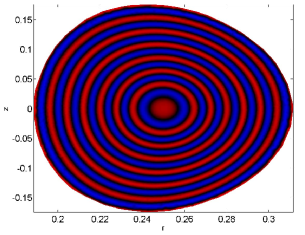
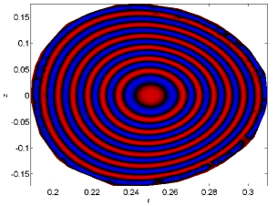
Figure 2: Visualization of ergodic partition on $\theta=0$ plane for the Poincare map of system (28); (a) $\epsilon=0.05$; (b) $\epsilon=0.01$

V Conclusions

In conclusion, we have proved the persistence of two-dimensional invariant tori in the perturbation of integrable action-angle-angle maps with degenerate angle. The persistence proof requires a combination of the proof techniques for non-degenerate volume-preserving maps as pursued in [15] and Arnold’s methods in proving the KAM theorem in the case of Hamiltonian systems with degenerate angles [2, 3]. A specific peculiarity of our proof is the need for an intermediate sequence of coordinate transformations that reduces the size of the perturbation in the action variable by an order and allows us to proceed with a Moser-type technique pursued in [15]. Elegant and shorter proof technique for KAM-type results has recently been pursued by Broer, Huitema and Sevryuk [9]. It would be interesting to see whether their “parametric” KAM-type technique could be used to prove a version of our theorem in a simpler way. In addition, we have used the main result of this paper to prove persistence of invariant tori in a perturbation of a volume-preserving Euler fluid flow, swirling Hill’s vortex, under the assumption of large swirl. Note that our proof above can be easily extended to the full class of perturbation similar to the single-mode perturbation in $\theta$ that we have used, as any such perturbation can be expanded in Fourier series. In other words, any sufficiently small, volume-preserving perturbation that has axial (z) symmetry will have a set of tori preserved.

VI Acknowledgement

The authors would like to acknowledge the help of Marko Budišić, from the University of California, Santa Barbara for providing the code and generating the plots for the ergodic partition of the three dimensional map in section IV. We thank an anonymous referee of the previous version for pointing out a problem with the proof. This research has been supported by ONR MURI grant.

References

- [1] A. N. Kolmogorov, 1954, On the conservation of conditionally periodic motions for a small change in Hamiltonian’s function, Doklady Akad. Nauk. SSSR. 98 p 527-530.
- [2] V. I. Arnold, 1963, Proof of a theorem of A. N. Kolmogorov on the preservation of conditionally periodic motions under a small perturbation of the Hamiltonian, Russian Mathematical Surveys 18, no. 5, p 9-36.
- [3] V. I. Arnold, 1963, Small denominator and problem of stability of motion in classical and celestial mechanics, Russian Mathematical Surveys 18, no.6, p 85-191.
- [4] J. Moser, 1962, On invariant curves of area-preserving mappings of an annulus Nachr. Akad. Wiss. Gottingen Math Phys. K1.II, p 1-20.
- [5] C. Siegel and J. Moser, Lectures on Celestial Mechanics Berlin Heidelberg: Springer- Verlag, 1971.
- [6] I. Mezić and S. Wiggins, 1994, On the integrability and perturbation of three-dimensional fluid flow with symmetry J. Nonlinear Sci. 4, p 157-194.
- [7] R. de la Llave, Recent progress in classical mechanics. Mathematical Physics, X (Leipzig 1991) Berlin Heidelberg: Springer-Verlag 1992.
- [8] H.W. Broer, G. B. Huitema and F. Takens, 1990, Unfolding of quasi-periodic tori Mem. Amer. Math. Soc. 421, p 1-82.
- [9] H. W. Broer, G. B. Huitema and M. B. Sevryuk, 1996, Quasi-periodic motion in the families of dynamical systems: order amidst chaos, Lectures notes in Mathematics 1645 Berlin Heidelberg: Springer-Verlag.
- [10] A. Delshams and R. de la Llave, 1991, Existence of quasi-periodic orbits and absence of transport for volume-preserving transformations and flow Preprint.
- [11] C. Q. Cheng and Y. Sun, 1994, Existence of KAM tori in degenerate Hamiltonian systems Journal of Differential Equations 114, p 288-335.
- [12] Z. H. Xia, 1992, Existence of invariant tori in volume-preserving diffeomorphisms Ergodic Theory and Dynamical Systems 12, p 621-631.
- [13] Zhu Wen-Zhuang and Huang Qing-Dao and Liu Bai-Feng, 2004, The persistence of invariant tori in nearly small twist mappings with intersection property Northeast Math. J. 20, no.2, p 175-190.
- [14] Y. Li and Y. Yi, 2002, Persistence of invariant tori in generalized Hamiltonian systems Ergodic theory and Dynamical Systems 22, p 1233-1261.
- [15] C. Q. Cheng and Y. Sun, 1990, Existence of invariant tori in three-dimensional measure preserving mappings Celestial Mechanics 47, p 275-292.
- [16] Xia Zhihong, 1995, Existence of invariant tori for certain non-symplectic diffeomorphism, Hamiltonian Dynamical Systems: History, Theory and Application New York: Springer.
- [17] H. W. Broer, 1981, Formal normal form theorems for fields and some consequences of bifurcations in the volume preserving case Lecture Notes in Mathematics 898 Springer-Verlag, p 54-74.
- [18] G. Haller and I. Mezić, 1998, Reduction of three-dimensional volume preserving flow with symmetry Nonlinearity 11, p 319-339.
- [19] O. Piro and M. Feingold, 1998, Diffusion in three-dimensional Liouvillian maps Phys. Rev. Lett. 61, p 1799-1802.
- [20] I. Mezić, 2001, Break-up of invariant surfaces in action-angle-angle maps and flow Physica D 154, p 51-67.
- [21] H. Whitney, 1934, Analytic extensions of differentiable functions defined in closed sets Trans. Amer. Math. Soc. 36, p 63-89.
- [22] E. M. Stein, 1970, Singular integrals and differentiability properties of functions Princeston New Jersey: Princeton University Press.
- [23] T. H. Solomon and I. Mezić, 2003, Uniform resonant chaotic mixing in fluid flows Nature 425, no. 6956, p 376-380.
- [24] I. Mezić, 1994, On Geometrical and Statistical Properties of Dynamical Systems: Theory and Applications, PhD Thesis, California Institute of Technology.
- [25] I. Mezić and S. Wiggins, 1999, A method for visualization of invariants sets of dynamical systems based on ergodic partition, Chaos Vol. 9, no. 1, p 213-218.
- [26] M. Budišić and I. Mezić, 2012, Geometry of the ergodic quotient reveals coherent structures in flows Accepted for publication in Physica D.
- [27] Z. Levanajić and I. Mezić, 2010, Ergodic theory and visualization I: Mesochronic plots for visualization of ergodic partition and invariant sets, Chaos Vol. 20, no. 3. p (033114) 1-19.