Fast and Simple Method for Pricing Exotic Options using Gauss-Hermite Quadrature on a Cubic Spline Interpolation

Abstract

There is a vast literature on numerical valuation of exotic options using Monte Carlo, binomial and trinomial trees, and finite difference methods. When transition density of the underlying asset or its moments are known in closed form, it can be convenient and more efficient to utilize direct integration methods to calculate the required option price expectations in a backward time-stepping algorithm. This paper presents a simple, robust and efficient algorithm that can be applied for pricing many exotic options by computing the expectations using Gauss-Hermite integration quadrature applied on a cubic spline interpolation. The algorithm is fully explicit but does not suffer the inherent instability of the explicit finite difference counterpart. A ‘free’ bonus of the algorithm is that it already contains the function for fast and accurate interpolation of multiple solutions required by many discretely monitored path dependent options. For illustrations, we present examples of pricing a series of American options with either Bermudan or continuous exercise features, and a series of exotic path-dependent options of target accumulation redemption note (TARN). Results of the new method are compared with Monte Carlo and finite difference methods, including some of the most advanced or best known finite difference algorithms in the literature. The comparison shows that, despite its simplicity, the new method can rival with some of the best finite difference algorithms in accuracy and at the same time it is significantly faster. Virtually the same algorithm can be applied to price other path-dependent financial contracts such as Asian options and variable annuities.

Keywords: exotic options, Gauss-Hermite quadrature, cubic spline, finite difference method, American option, Bermudan option, target accumulation redemption note (TARN), GMWB variable annuity

¹ The Commonwealth Scientific and Industrial Research Organisation, Australia
e-mail: Xiaolin.Luo@csiro.au
² The Commonwealth Scientific and Industrial Research Organisation, Australia
e-mail: Pavel.Shevchenko@csiro.au

1 Introduction

There is a vast literature on numerical valuation of exotic options using Monte Carlo, trees and partial differential equation methods. For text book treatment of this topic, see Wilmott (2007) and Hull (2009); also more specialized books Glasserman (2004) for Monte Carlo and Tavella and Randall (2000) for finite difference methods. The choice of method is dictated by the type of option and underlying asset stochastic process. For example, for pricing American type option the modeller can use finite difference or tree methods in the case of one or two underlying assets and the Least-Squares Monte Carlo (LSMC) method (Longstaff and Schwartz (2001)) for higher dimensions; for pricing basket options without early exercise features the modeller can use standard Monte Carlo; etc. It is also worth mentioning that for contracts where the underlying asset process depends on the contract control variables (e.g. variable annuities with guaranteed minimum withdrawal benefit where the underlying wealth process is affected by optimal cash withdrawals that should be found from backward solution), the underlying process cannot be simulated forward in time and thus the standard LSMC method cannot be applied.

In the case when transition density of the underlying asset between time slices or its moments are known in closed form and problem dimension is low (one or two underlying stochastic variables), often it can be convenient and more efficient to utilize direct integration methods to calculate the required option price expectations in backward time-stepping algorithm. In this paper, we present a method that relies on computing the expectations in backward time-stepping through Gauss-Hermite integration quadrature applied on a cubic spline interpolation; we use GHQC (Gauss-Hermite quadrature on Cubic-spline) to denote this method. We show that the GHQC can be made fully explicit, so it is as fast as an explicit finite difference algorithm but at the same time it is more accurate and does not suffer the inherent instability of the latter. This approach can be applied to numerical valuation of many exotic options including barrier, Asian and American type options, and contracts written on the asset with path affected by optimal control variables such as variable annuity with guaranteed minimum withdrawal benefit. In general, it can be applied to any option that can be evaluated using finite difference method if the underlying asset transition density or its moments are easily evaluated. It is easy to implement and understand. Also, in general the accuracy of GHQC can rival the widely used semi-implicit second order finite difference algorithm, but GHQC is much faster because it either requires less number of time steps or it is faster per time step due to its full explicitness. Of course the number of time steps depends on time discretisation required by stochastic process and option contract details (e.g. barrier or early exercise monitoring frequency).

We first describe GHQC algorithm in details and then illustrate the use of the algorithm to compute American options and the path-dependent TARN options. Two series of American options are considered - one with discrete exercise (so called Bermudan option) and another one with continuous exercise in time. The results of GHQC are compared with those by several finite difference algorithms and LSMC method. The comparison includes some of the most sophisticated and advanced finite difference algorithms found in the literature (Brennan and Schwartz (1977), Wilmott et al. (1995), Leisen and Reimer (1996), Wu and Kwok (1997), Forsyth et al. (2002), Nielsen et al. (2002), Han and Wu (2004), Ikonen and Toivanen (2004), Borici and Lüthi (2005), and Tangman et al. (2008)), and it demonstrates the good accuracy and high efficiency of the algorithm.

It is straightforward to apply the algorithm (with similar benefits) to barrier options, Asian options, targeted accrual redemption notes (TARNs) and variables annuities. This is demonstrated by pricing a series of twelve TARN contracts covering three “knockout” types and four accumulation target levels. The results are compared with those of finite difference and Monte Carlo, which again illustrates the robustness, accuracy and efficiency of the GHQC algorithm. Of course it is expected that in high dimensions the Monte Carlo method will be more efficient (standard MC for options without early exercise and LSMC for American type options). For application of the algorithm for pricing variable annuities with GMWB and death benefit, see Luo and Shevchenko (2014a, c).

2 Model

Let $S(t)$ denote the value of the option underlying asset that follows the risk-neutral stochastic process

$$dS(t)=\mu(t)S(t)dt+\sigma(t)S(t)dB(t),$$ (1)

where $\mu(t)$ is the drift (i.e. it is the risk-free interest rate $r(t)$ minus dividends if $S(t)$ is equity or difference between domestic and foreign interest rates if $S(t)$ is foreign exchange), $\sigma(t)$ is the volatility and $B(t)$ is a standard Brownian motion. The risk free interest rate $r(t)$ can be function of time. The drift and volatility can be functions of time and underlying asset but for illustrative examples we assume that drift and volatility are functions of time only.

In this paper we do not consider time discretization errors; for simplicity, hearafter, we assume that model parameters are piece-wise constant functions of time for discretization $0=t_{0}<t_{1}<\cdots<t_{N}=T$, where $T$ is contract maturity. Denote corresponding asset values as $S(t_{0}),S(t_{1}),\ldots,S(t_{N})$; and drift, risk-free interest rate and volatility as $\mu_{1},\ldots,\mu_{N}$, $r_{1},\ldots,r_{N}$ and $\sigma_{1},\ldots,\sigma_{N}$ respectively. That is $\mu_{1}$ is the drift for time period $(t_{0},t_{1}]$; $\mu_{2}$ is for $(t_{1},t_{2}]$, etc. and similar for risk-free interest rate and volatility. To simplify notation, we also assume that the monitoring frequency specific to the option contract corresponds to the same time discretization. For example, barrier monitoring dates or Bermudan exercise dates or Asian averaging dates are the same as the time discretization. It is trivial extension if monitoring dates reside on some time slices only so that there are time steps between the monitoring dates.

Denote the transition density function from $S(t_{n-1})$ to $S(t_{n})$ as $p_{n}(s(t_{n})|s(t_{n-1}))$, which is just a lognormal density in the case of process (1) with solution

$$S(t_{n})=S(t_{n-1})e^{(\mu_{n}-\frac{1}{2}\sigma_{n}^{2})dt_{n}+\sigma_{n}\sqrt{dt_{n}}z_{n}},\;\;n=1,2,\ldots,N,$$ (2)

where $dt_{n}=t_{n}-t_{n-1}$ and $z_{1},\ldots,z_{N}$ are independent and identically distributed random variables from the standard Normal distribution. That is, distribution of $\ln S(t_{n})$ conditional on $\ln S(t_{n-1})$ is Normal with the mean $\ln S(t_{n-1})+(\mu_{n}-\frac{1}{2}\sigma_{n}^{2})dt_{n}$ and standard deviation $\sigma_{n}\sqrt{dt_{n}}$.

In general, the today’s fair price of the option can be calculated as expectation of discounted option payoff with respect to the risk neutral process (1), given information today at $t_{0}$, and typically can be found via backward time stepping by calculating option price $Q_{n}(S(t_{n}))$ at each $t_{n}$ that requires evaluation of conditional expectations (conditional on information at $t_{n-1}$)

$$\widetilde{Q}_{n-1}(S(t_{n-1}))=\mathrm{E}_{t_{n-1}}\left[e^{-r_{n}dt_{n}}{Q_{n}}\left(S(t_{n})\right)\right],$$ (3)

and applying some jump or early exercise condition specific to the option. If no condition is applied then $\widetilde{Q}_{n-1}$ equals ${Q}_{n-1}$. Expectation (3) can be written explicitly as the following integral

$$\widetilde{Q}_{n-1}(S(t_{n-1}))=\int_{0}^{+\infty}e^{-r_{n}dt_{n}}p_{n}\left(s|S(t_{n-1})\right)Q_{n}(s)ds.$$ (4)

The objective of the GHQC algorithm is to evaluate these integrals efficiently. These integrations occur in many path-dependent options. Below we explicitly show this for Bermudan, barrier, Asian, a target accumulation redemption note (TARN) and variable annuity with Guaranteed Minimum Withdraw Benefit (GMWB).

2.1 Bermudan option

Consider Bermudan option with early exercise dates the same as time discretization $0=t_{0}<t_{1}<\cdots<t_{N}=T$. Then the option value at $t=0$ is calculated recursively backward in time as

$$Q_{n-1}(S(t_{n-1}))=\max\left(\widetilde{Q}_{n-1}(S(t_{n-1})),\max\left(0,\phi\times(S(t_{n-1})-K)\right)\right),$$ (5)

starting from

$$Q_{N}(S(T))=\max(0,\phi\times(S(T)-K)),$$

where $\widetilde{Q}_{n-1}(S(t_{n-1}))$ is given by (4), $K$ is the strike, $\phi=1$ for call option and $\phi=-1$ for put option. In the limit of continuous early exercise ($N\rightarrow\infty$), this option is called American option.

2.2 Barrier option

Consider barrier option with piece-wise constant barriers with time discretization $0=t_{0}<t_{1}<\cdots<t_{N}=T$. Denote the lower and upper barriers as $L_{1},\ldots,L_{N}$ and $U_{1},\ldots,U_{N}$ respectively, where $L_{1}$ is the lower barrier for time period $[t_{0},t_{1}]$; $L_{2}$ is for $(t_{1},t_{2}]$, etc. and similar for the upper barrier. Then the knockout barrier option value at $t=0$ is calculated recursively backward in time as

$$Q_{n-1}(S(t_{n-1}))=\widetilde{Q}_{n-1}(S(t_{n-1}))$$

$$\quad=\int_{L_{n}}^{U_{n}}e^{-r_{n}dt_{n}}p_{n}\left(s|S(t_{n-1})\right)g_{n}(S(t_{n-1}),s)Q_{n}(s)1_{(L_{n},U_{n})}(S(t_{n-1}))ds$$ (6)

starting from

$$Q_{N}(S(T))=\max(0,\phi\times(S(T)-K)),$$

where $K$ is the strike, $\phi=1$ for knockout call option and $\phi=-1$ for knockout put option, and $1_{\mathcal{A}}(x)$ is indicator function equal 1 if $x\in\mathcal{A}$ and $0$ otherwise. $g_{n}(s_{n-1},s_{n})$ is probability of no barrier hit within $[t_{n-1},t_{n}]$ conditional on asset taking values $s_{n-1}$ and $s_{n}$ at $t_{n-1}$ and $t_{n}$ respectively with $s_{n-1}\in(L_{n},U_{n})$ and $s_{n}\in(L_{n},U_{n})$; it is the so-called Brownian bridge correction often used in the literature on pricing barrier options, see e.g. Andersen and Brotherton-Racliffe (1996); Shevchenko (2003); Beaglehole et al. (1997); Shevchenko and Del Moral (2014). In the case of discrete barrier monitoring (i.e. no barrier during $(t_{n-1},t_{n})$), $g_{n}(s_{n-1},s_{n})=1$ if both $s_{n–1}$ and $s_{n}$ are between the barriers and zero otherwise; in the case of single continuous barrier $B_{n}$ (either lower or upper) during $[t_{n-1},t_{n}]$

$$g_{n}(s,s^{\prime})=1-\exp\left(-2\frac{\ln(s^{\prime}/B_{n})\ln(s/B_{n})}{\sigma^{2}_{n}dt_{n}}\right);$$ (7)

and there is a closed form solution for the case of continuous double barrier within $[t_{n-1},t_{n}]$

$$g_{n}(s,s^{\prime}) = 1-\sum_{m=1}^{\infty}[R_{n}\left(\alpha_{n}m-\gamma_{n},x_{n}\right)+R_{n}(-\alpha_{n}m+\beta_{n},x_{n})]$$ (8)

$$+\sum_{m=1}^{\infty}[R_{n}(\alpha_{n}m,x_{n})+R_{n}(-\alpha_{n}m,x_{n})],$$

where

$$x_{n}=\ln\frac{s^{\prime}}{s},\alpha_{n}=2\ln\frac{U_{n}}{L_{n}},\beta_{n}=2\ln\frac{U_{n}}{s},\gamma_{n}=2\ln\frac{s}{L_{n}},R_{n}(z,x)=\exp\left(-\frac{z(z-2x)}{2\sigma^{2}_{n}\delta t_{n}}\right).$$

If either $s$ or $s^{\prime}$ breaches the barrier condition, then we get set $g(s,s^{\prime})=0$. Typically only a few terms in summations in (8) are required to achieve good accuracy for option price estimator.

2.3 Asian option

Consider a discretely monitored Asian option with the standard arithmetic average defined over the monitoring times $t_{1},\ldots,t_{n}$ as

$$A(t_{n})=\frac{1}{n}\sum_{i=1}^{n}S(t_{i}).$$

Between monitoring times, i.e. for $t\in(t_{n-1},t_{n})$, the arithmetic average is $A(t)=A(t_{n-1})$ and the option value $Q(S(t),A(t))$ can be evaluated as

$$Q(S(t),A(t))={\widetilde{Q}}(S(t),A(t))=\int_{0}^{+\infty}e^{-r_{n}(t_{n}-t)}p_{n}\left(s|S(t)\right)Q_{n}(s(t_{n}^{-}),A(t_{n}^{-}))ds,$$ (9)

where $t_{n}^{-}$ denotes the time immediately before the monitoring time $t_{n}$. Let $t_{n-1}^{+}$ denote the time immediately after the monitoring time $t_{n-1}$, then the option value $Q_{n-1}(S(t_{n-1}^{+}),A(t_{n-1}^{+}))$ can be calculated from (9) by letting $t=t_{n-1}^{+}$ . The option value immediately before $t=t_{n-1}$, $Q_{n-1}(S(t_{n-1}^{-}),A(t_{n-1}^{-}))$, can then be obtained through a special jump condition reflecting the continuity of option value and the finite change in the arithmetic average across from $t_{n-1}^{-}$ to $t_{n-1}^{+}$:

$$Q_{n-1}(S(t_{n-1}^{-}),A(t_{n-1}^{-}))={\widetilde{Q}}_{n-1}\left(S(t_{n-1}^{-}),A(t_{n-1}^{-})+\frac{S(t_{n-1}^{-})-A(t_{n-1}^{-})}{n-1}\right),$$ (10)

where $A(t_{n-1}^{-})=A(t_{n-2})=\frac{1}{n-2}\sum_{i=1}^{n-2}S(t_{i})$ and of course $S(t_{n-1}^{-})=S(t_{n-1}^{+})=S(t_{n-1})$. Repeatedly applying (9) and (10) backwards gives us the option value at $t=0$, starting from

$$Q_{N}(S(T),A(T))=\max(0,\phi\times(S(T)-A(T)).$$

Note that formula (9) is for a given fixed value of $A$, while the jump condition (10) implies that across any monitoring time the average $A$ jumps to arbitrarily different values depending on the values of $A$ and the asset value $S$, which means in principle we have to track multiple solutions corresponding to all possible values of $A$. Numerically, this can be done by discretizing the average space $A$, similar to discretizing the asset space $S$. Interpolating multiple solutions of different values of $A$ enables us to apply the jump condition at all monitoring times.

2.4 TARN

Consider TARN contract that provides a capped sum of payment (target cap) over a period with the possibility of early termination. Let $U$ be the target accrual level and $A_{n}=\sum_{i=1}^{n}\max(0,\phi\times(S(t_{i})-K)))$ is the accumulated amount on the fixing date $t_{n}$. Later we will show numerical results of pricing TARN contracts with three different “knockout” types used in practice:

• Full gain – when the target is breached on a fixing date $t_{n}$, the cash flow payment on that date is allowed. This essentially permits the breach of the target once, and the total payment may exceed the target for full gain knockout.

• No gain – when the target is breached, the entire payment on that date is disallowed. The total payment will never reach the target for no gain knockout.

• Part gain – when the target is breached on a fixing date $t_{n}$, part of the payment on that date is allowed, such that the target is met exactly.

In the case of “full gain” knockout TARN, the present value (discounted value at $t_{0}=0$) of the TARN payoff $P^{(\text{Full})}$ is

$$P^{(\text{Full})}=\sum_{i=1}^{\widetilde{N}}e^{-rt_{i}}\max(0,\phi\times(S(t_{i})-K))),$$

where $r=(r_{1}dt_{1}+\cdots+r_{i}dt_{i})/t_{i}$ and $1\leq{\widetilde{N}}\leq N$ is the first time the target $U$ is breached by $A_{n}$. In the case of “no gain”, the last payment is disallowed, thus the payoff $P^{(\text{No gain})}$ is

$$P^{(\text{No gain})}=\sum_{i=1}^{{\widetilde{N}}-1}e^{-rt_{i}}\max(0,\phi\times(S(t_{i})-K))),$$

and in the case of “part gain”, we have payoff $P^{(\text{Part})}$ given as

$$P^{(\text{Part})}=P^{(\text{No gain})}+e^{-rt_{\widetilde{N}}}\times(U-P^{(\text{No gain})}).$$

The price evolution of TARN between payment dates can also be expressed by (9), the same as for the Asian option. However, the jump condition across a payment date now becomes

$$Q_{n-1}(S(t_{n-1}^{-}),A(t_{n-1}^{-}))={\widetilde{Q}}_{n-1}\left(S(t_{n-1}),A(t_{n-1}^{+})\right)+\max(0,\phi\times(S(t_{n-1})-K)),$$ (11)

where $A(t_{n-1}^{+})=A(t_{n-1}^{-})+\max(0,\phi\times(S(t_{n-1})-K))$, and $A(t_{n-1}^{-})=A(t_{n-2}^{+})<U$. Obviously, similar to the Asian option, tracking of multiple solutions corresponding to different accumulated amount $A_{n}$ is required and thus interpolation between them is necessary. For numerical valuation of TARN contracts via Monte Carlo and finite difference methods, see Piterbarg (2004) and Luo and Shevchenko (2014b).

2.5 GMWB

Guaranteed Minimum Withdraw Benefit is one of the most popular variable annuity contracts in practice, see e.g. Dai et al. (2008) and Luo and Shevchenko (2014a, c). A GMWB contract promises to return the entire initial investment through cash withdrawals during the policy life plus the remaining account balance at maturity, regardless of the portfolio performance. Assume the entire initial premium $W(0)$ is invested in asset $S$, and at each withdraw date $t_{n}$ the amount $\gamma_{n}$ is withdrawn. Then the account balance of the guarantee $A(t)$ with $A(0)=W(0)$ evolves as

$$A(t_{n})=A(t_{n}^{-})-\gamma_{n}=A(t_{n-1})-\gamma_{n},\;\;n=1,2,\ldots,N$$ (12)

with $A(T)=0$, $W(0)=A(0)\geq\gamma_{1}+\cdots+\gamma_{N}$ and $A(t_{n-1})=A(t_{n-1}^{+})\geq\sum_{i=n}^{N}\gamma_{i}$. The value of personal variable annuity account $W(t)$ evolves as

$$W(t_{n})=\max\left[W(t_{n-1})e^{(\mu_{n}-\alpha-\frac{1}{2}\sigma_{n}^{2})dt_{n}+\sigma_{n}\sqrt{dt_{n}}z_{n}}-\gamma_{n},0\right]\;\;n=1,2,\ldots,N,$$ (13)

where $dt_{n}=t_{n}-t_{n-1}$, $z_{n}$ are independent and identically distributed random variables from the standard Normal distribution and $\alpha$ is the annual fee. If the account balance becomes zero or negative, then it will stay zero till maturity.

The numerical algorithm for GMWB with discrete withdrawals is again very similar to Asian options described above, at least for the “static” or passive case where the withdraw amount $\gamma_{n}=G$ is a constant specified by the contract. The evolution of price between withdraw dates expressed by (9) still holds, provided the drift $\mu_{n}$ is replaced by $\mu_{n}-\alpha$ to account for the continuously charged fee $\alpha$. After the amount $\gamma_{n}$ is drawn at $t_{n}$, the annuity account reduces from $W(t_{n}^{-})$ to $W(t_{n})=\max(W(t_{n}^{-})-\gamma_{n},0)$, and the jump condition of $Q_{n}(W,A,t)$ across $t_{n}$ is given by

$$Q_{n-1}\left(W(t_{n}^{-}),A(t_{n}^{-})\right)={\widetilde{Q}}_{n-1}\left(\max(W(t_{n}^{-})-\gamma_{n},0),A(t_{n}^{-})-\gamma_{n}\right)+\gamma_{n}.$$ (14)

Repeatedly applying (9) and (14) backwards gives us the contract value to $t=0$, starting from the final condition

$$Q_{N}(W(T^{-}),A(T^{-}))=\max\left(W(T^{-}),A(T^{-})\right).$$

For the dynamic (optimal) withdraw case, the policyholder may decide to withdraw above or below the contractual rate to maximize the present value of the total cash flow generated from holding the GMWB contract, and in such a case a penalty is applied by the insurer and the net cash received by the policyholder for each withdraw $\gamma$ becomes $c(\gamma)$ which may be less than $\gamma$:

$$c(\gamma)=\left\{\begin{array}[]{ll}\gamma,&\mbox{if}\;0\leq\gamma\leq G,\\ G+(1-\beta)(\gamma-G),&\mbox{if}\;\gamma>G,\end{array}\right.$$ (15)

and the jump condition for the optimal withdraw case now can be written as

$$Q_{n}\left(W(t_{n}^{-}),A(t_{n}^{-})\right)=\max_{0\leq\gamma_{n}\leq A(t_{n}^{-})}\left[{\widetilde{Q}}_{n}\left(\max(W(t_{n}^{-})-\gamma_{n},0),A(t_{n}^{-})-\gamma_{n}\right)+c(\gamma_{n})\right],$$ (16)

That is, at each withdraw date $t=t_{n}$ the policyholder ‘optimally’ withdraws an amount $\gamma_{n}$ to maximize the option value. The final condition for the dynamic case is given by

$$Q_{N}(W(T^{-}),A(T^{-}))=\max\left(W(T^{-}),c\left(A(T^{-})\right)\right).$$

3 The GHQC Method

The few path-dependent options described in the previous section all require the evaluation of expectation (3). The most widely used methods for calculating this expectation are pde solutions and Monte Carlo simulations, and a possible alternative is the direct numerical integration of (4), a recent example of this approach can be found in Aluigi et al. (2014).

Except the American and barrier options, all the other examples described in the last section require accurate interpolation of multiple solutions. As shown in a convergence study by Forsyth et al. (2002), it is possible for a numerical algorithm of discretely sampled path-dependent option pricing to be non-convergent (or convergent to an incorrect answer) if the interpolation scheme is selected inappropriately. Typically previous studies of numerical pde solution for path-dependent (Asian or lookback options) used either a linear or a quadratic interpolation in applying the jump conditions.

Below we propose a simple, robust and efficient algorithm for integrating (4) in the context of path-dependent option pricing, and at the same time the proposed algorithm also naturally (as a byproduct) provides an accurate and efficient procedure for interpolating multiple solutions at little extra computing cost.

3.1 Numerical evaluation of the expectation

Similar to a finite difference scheme, we propose to discretize the asset domain $(S_{\min},S_{\max})$ by $S_{\min}=S_{0}<S_{1},\ldots,S_{M}=S_{\max}$ , where $S_{\min}$ and $S_{\max}$ are the lower and upper boundary, respectively, both are sufficiently far from the spot asset value at time zero $S(0)$. A reasonable choice of such boundaries could be $S_{\max}=S(0)\exp(5\sigma\sqrt{T})$ and $S_{\min}=S(0)\exp(-5\sigma\sqrt{T})$ (a better choice will be given later in (35)). The idea (from finite difference method) is to find option values at all these grid points at all time slices $0=t_{0}<t_{1}<\ldots<t_{N}=T$ through backward time stepping, starting at maturity $t=t_{N}=T$, and at each time step we evaluate the integration (4) for every grid point by a high accuracy numerical quadrature.

The option value at $t=t_{n}$ is known only at grid points $S_{m}$, $m=0,1,\ldots,M$. In order to approximate the continuous function $Q_{n}(S(t_{n}))$ from the values at the discrete grid points, and perform the required integration, we propose to use the cubic spline interpolation which is smooth in the first derivative and continuous in the second derivative (Press et al. (1992)). The error of cubic spline is $O(h^{4})$, where $h$ is the size for the spacing of the interpolating variable, assuming a uniform spacing. Given any arbitrary tabulated function $Q(x_{j}),\;j=0,\ldots,M$, the value of $Q(x),\;x_{j}<x<x_{j+1}$, can be approximated by the cubic spline interpolation

$$Q(x)\approx AQ(x_{j})+BQ(x_{j+1})+CQ^{\prime\prime}(x_{j})+DQ^{\prime\prime}(x_{j+1}),$$ (17)

where

$$A=\frac{x_{j+1}-x}{x_{j+1}-x_{j}},\;\;B=1-A,$$

$$C=(A^{3}-A)(x_{j+1}-x_{j})^{2}/6,\;\;D=(B^{3}-B)(x_{j+1}-x_{j})^{2}/6.$$

From a continuity condition, the second derivatives are obtained by solving the following tri-diagonal system of linear equations (Press et al. (1992))

$$\frac{dx_{j}}{6}Q^{\prime\prime}(x_{j-1})+\frac{x_{j+1}-x_{j-1}}{3}Q^{\prime\prime}(x_{j})+\frac{dx_{j+1}}{6}Q^{\prime\prime}(x_{j+1})$$

$$\quad\quad\quad\quad\quad\quad\quad=\frac{Q(x_{j+1})-Q(x_{j})}{dx_{j+1}}-\frac{Q(x_{j})-Q(x_{j-1})}{dx_{j}},$$ (18)

where $\;j=1,\ldots,M-1$,$dx_{j}=x_{j}-x_{j-1}$, $dx_{j+1}=x_{j+1}-x_{j}$. For boundary conditions we can set $Q^{\prime\prime}(x_{0})=Q^{\prime\prime}(x_{M})=0$ (natural boundary condition), which is consistent with the boundary condition of zero second-derivatives for option values at far boundaries. Other boundary conditions are possible, depending on the option specifics. For a fixed grid, the tri-diagonal matrix can be inverted once and at each time step only the back-substitution in the cubic spline procedure is required. Cubic spline functions are available in most numerical packages and are very easy to use.

For the lognormal stock process, the distribution of $S(t_{n})$ given $S(t_{n-1})$ is a lognormal distribution corresponding to solution (2). A convenient and common practice is to work with $\ln(S(t_{n}))$ so that the corresponding conditional density is Normal distribution with the mean $\ln S(t_{n-1})+(\mu_{n}-\frac{1}{2}\sigma_{n}^{2})dt_{n}$ and standard deviation $\sigma_{n}\sqrt{dt_{n}}$. In order to make use of the highly efficient Gauss-Hermite numerical quadrature for integration over an infinite domain, for each time slice, we introduce a new variable

$$Y(t_{n})=\frac{\ln\left(S(t_{n})/S(t_{n-1})\right)-\nu_{n}}{\tau_{n}},$$ (19)

where $\nu_{n}=(\mu_{n}-\frac{1}{2}\sigma_{n}^{2})dt_{n}$ and $\tau_{n}=\sigma_{n}\sqrt{dt_{n}}$, and denote the option price function $Q_{n}(s)$ after this transformation as $Q_{n}^{(y)}(y)$. By changing variable from $S(t_{n})$ to $Y(t_{n})$ the integration (4) becomes

$$\widetilde{Q}_{n-1}(S(t_{n-1}))=\frac{e^{-r_{n}dt_{n}}}{\sqrt{2\pi}}\int_{-\infty}^{+\infty}e^{-\frac{1}{2}y^{2}}Q_{n}^{(y)}(y)dy.$$ (20)

For such integrals the Gauss-Hermite integration quadrature is well known to be very efficient (Press et al. (1992)). For an arbitrary function $f(x)$, the Gauss-Hermite quadrature is

$$\int_{-\infty}^{+\infty}e^{-x^{2}}f(x)dx\approx\sum_{j=1}^{q}\lambda_{j}^{(q)}f(\xi_{j}^{(q)}),$$ (21)

where $q$ is the order of the Hermite polynomial, $\xi_{j}^{(q)}$ are the roots of the Hermite polynomial $H_{q}(x)(j=1,2,\ldots,q)$, and the associated weights $\lambda_{j}^{(q)}$ are given by

$$\lambda_{j}^{(q)}=\frac{2^{q-1}q!\sqrt{\pi}}{q^{2}[H_{q-1}(\xi_{j}^{(q)})]^{2}}.$$

As a reference the abscissas (roots) and the weights for $q=6,\;6$ and $16$ are given in the Appendix. In general, the abscissas and the weights for the Gauss-Hermite quadrature for a given order $q$ can be readily computed, e.g. using the functions in Press et al. (1992).

Applying a change of variable $x=y/\sqrt{2}$ and use the Gauss-Hermite quadrature to (20), we obtain

$$\widetilde{Q}_{n-1}(S(t_{n-1}))=\frac{e^{-r_{n}dt_{n}}}{\sqrt{\pi}}\int_{-\infty}^{+\infty}e^{-x^{2}}Q_{n}^{(y)}(\sqrt{2}x)dx\approx\frac{e^{-r_{n}dt_{n}}}{\sqrt{\pi}}\sum_{j=1}^{q}\lambda_{j}^{(q)}Q_{n}^{(y)}(\sqrt{2}\xi_{j}^{(q)}).$$ (22)

If we apply the change of variable (19) and the Gauss-Hermite quadrature (22) to every grid point $S_{m}$, $m=0,1,\ldots,M$, i.e. let $S(t_{n-1})=S_{m}$, then the option values at time $t=t_{n-1}$ for all the grid points can be evaluated through (22).

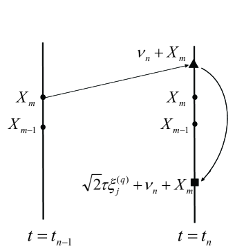
Figure 1: Illustration of Gauss-Hermite quadrature application for an arbitrary grid point $X_{m}$ at time $t=t_{n-1}$. The solid circles are fixed grid points, the solid triangle is the point of the expected mean at $t=t_{n}$ given $X_{m}$ at $t=t_{n-1}$, and the solid square is the $j-th$ quadrature point corresponding to $X_{m}$.

It is a common practice in a finite difference setting for option pricing to set the working domain in asset space in terms of $X=\ln(S/S(0))$, where $S(0)$ is the spot value at time $t=0$. The domain $(X_{\min},X_{\max})$ is uniformly discretised to yield the grid $(X_{\min}=X_{0},X_{1}=\delta X,X_{2}=2\delta X,\ldots,X_{M}=M\delta X=X_{\max})$, where $\delta X=(X_{\max}-X_{\min})/M$. The grid point $S_{m}$, $m=0,1,\ldots,M$, is then given by $S_{m}=S(0)\exp(X_{m})$. The boundaries $X_{\min}=\ln(S_{\min}/S(0))$ and $X_{\max}=\ln(S_{\max}/S(0))$ have to be set sufficiently far from spot value to ensure the adequacy of applying far boundary conditions.

For each grid point $S_{m}$ or $X_{m}$, the variable $Y(t_{n})$ is given by (19) with $S(t_{n-1})=S_{m}$, and the relationship between $X(t_{n})=\ln(S(t_{n})/S(0))$ and $Y(t_{n})$ for $S_{m}$ is worked out to be $X(t_{n})=\tau_{n}Y(t_{n})+\nu_{n}+X_{m}$, thus the numerical integration value for grid point $X_{m}$ at time $t_{n-1}$ can be expressed, from (22), as

$$\widetilde{Q}_{n-1}^{(x)}(X_{m})\approx\frac{e^{-r_{n}dt_{n}}}{\sqrt{\pi}}\sum_{j=1}^{q}\lambda_{j}^{(q)}Q_{n}^{(x)}(\sqrt{2}\tau\xi_{j}^{(q)}+\nu_{n}+X_{m}).$$ (23)

where $Q_{n}^{(x)}(X(t_{n}))$ denotes the option value $Q_{n}(S(t_{n}))$ as a function of $X(t_{n})$ at time $t_{n}$. The continuous function $Q_{n}^{(x)}(\cdot)$ is approximated by the cubic spline interpolation, given the values $Q_{n}^{(x)}(X_{m})$ at discrete points $X_{m}$, $m=0,1,\ldots,M$. The above description of the numerical integration using Gauss-Hermite quadrature is illustrated in Figure 1.

Once the continuation value $\widetilde{Q}_{n-1}^{(x)}$ is known, then, in the case of Bermudan option, we get the option price at time $t=t_{n-1}$ as

$$Q_{n-1}^{(x)}(X_{m})=\max(\widetilde{Q}_{n-1}^{(x)}\left(X_{m}),\max(0,\phi\times(S_{m}-K)\right).$$ (24)

3.2 The GHQC algorithm for Bermudan options

The backward time-stepping algorithm using GHQC for evaluating the expectation (4) and Bermudan option price (5) can be summarized as follows

Algorithm 3.1 (GHQC)

• Step 1. Discretize the time domain and asset domain to have time grids $(0=t_{0}<t_{1}<\cdots<t_{N}=T)$ and asset grids (in terms of $X$) $(X_{\min}=X_{0}<X_{1}<\cdots<X_{M}=X_{\max})$, where $t_{n},\;\;n=1,2,\ldots,N$ are the exercise dates and $X_{m}=X_{m-1}+\delta X,\;\;\;\delta X=(X_{\max}-X_{\min})/M,\;\;m=1,2,\ldots,M$.

• Step 2. Take final payoff at maturity $t=t_{N}=T$ as the option price, i.e. $Q_{N}^{(x)}(X_{m})=\max(0,\phi\times(S_{m}-K)),\;\;m=0,1,\ldots,M$, where $S_{m}=S(0)\exp(X_{m})$.

• Step 3. Do cubic spline interpolation based on variable $X$ and the $M+1$ values $Q_{N}^{(x)}(X_{m}),\;\;m=0,1,\ldots,M$. This is done by first solving the tri-diagonal system of linear equations (3.1), with function values $Q_{N}^{(x)}(X_{m})$, and then use (17).

• Step 4. Do numerical integration for each grid point $X_{m}$ by Gauss-Hermite quadrature given in (23) to evaluate $\widetilde{Q}_{N-1}^{(x)}(X_{m}),\;\;m=0,1,2,\ldots,M$.

• Step 5. Apply early exercise test to obtain

  $$Q_{N-1}^{(x)}(X_{m})=\max(\widetilde{Q}^{(x)}_{N-1}\left(X_{m}),\max(0,\phi\times(S_{m}-K))\right).$$

• Step 6. Repeat Steps 3,4 and 5 for time steps $t=t_{N-2},t_{N-3},\ldots,t_{1}$.

• Step 7. Repeat Steps 3 and 4 for time step $t=t_{0}=0$, and take $\widetilde{Q}_{0}^{(x)}(0)$ as today’s option price.

The above GHQC algorithm has been implemented in $C$ computing language.

3.3 GHQC with moment matching

In calculation of option price expectations (20), the probability density function (transition density) for $Y(t_{n})$ is known in closed form; it is just standard Normal density. In general the closed form density function may not be known, and here we propose a moment matching to replace (20), i.e. assuming we do not know the density in closed form but we know the moments of the distribution, we can still use the GHQC algorithm by matching the numerically integrated moments with the known moments. Let $p(y)$ denote the unknown probability density function of $Y(t_{n})$, then (20) becomes

$$\widetilde{Q}_{n-1}(S(t_{n-1}))=e^{-r_{n}dt_{n}}\int_{-\infty}^{+\infty}p(y)Q_{n}^{(y)}(y)dy,$$ (25)

which can be re-written as

$$\widetilde{Q}_{n-1}(S(t_{n-1}))=e^{-r_{n}dt_{n}}\int_{-\infty}^{+\infty}e^{-y^{2}}\times[e^{y^{2}}p(y)]Q_{n}^{(y)}(y)dy.$$ (26)

Applying Gauss-Hermite quadrature (21) to (26) we then have

$$\widetilde{Q}_{n-1}(S(t_{n-1}))\approx e^{-r_{n}dt_{n}}\sum_{j=1}^{q}\lambda_{j}^{(q)}\widetilde{p}(\xi_{j}^{(q)})Q_{n}^{(y)}(\xi_{j}^{(q)}),$$ (27)

where the function $\widetilde{p}(y)=e^{y^{2}}p(y)$ is also unknown. Defining a new weight $W_{j}^{(q)}=\lambda_{j}^{(q)}\widetilde{p}(\xi_{j}^{(q)})$, the numerical quadrature for the integration simplifies to

$$\int_{-\infty}^{+\infty}p(y)Q_{n}^{(y)}(y)dy\approx\sum_{j=1}^{q}W_{j}^{(q)}Q_{n}^{(y)}(\xi_{j}^{(q)}).$$ (28)

Now we proceed to find the unknown coefficients $W_{j}^{(q)},\;j=1,2,\ldots,q$ by matching moments. Recognizing that if we replace $Q_{n}^{(y)}(y)$ by $y^{K}$, the integration yields the $K$-th moment corresponding to the pdf $p(y)$

$$\mathrm{E}_{t_{n-1}}[Y(t_{n})^{K}]=\int_{-\infty}^{+\infty}p(y)y^{K}dy\approx\sum_{j=1}^{q}W_{j}^{(q)}(\xi_{j}^{(q)})^{K}.$$ (29)

If we let $K=0,1,\ldots,q-1$ we then have $q$ equations to determine the $q$ unknown coefficients $W_{j}^{(q)},\;j=1,2,\ldots,q$.

In our American option evaluation framework the option value is a function of $X(t_{n})=\ln(S(t_{n})/S(0))$, and for each node point $X_{m}$ we have $X(t_{n})=\tau_{n}Y(t_{n})+\nu_{n}+X_{m}$. To match the central moment for random variable $X(t_{n})$ (centered at $\nu_{n}+X_{m}$), equation (29) becomes

$$\mathrm{E}_{t_{n-1}}[(X(t_{n})-\nu_{n}-X_{m})^{K}] = \int_{-\infty}^{+\infty}p_{X(t_{n})}(x)(x-\nu_{n}-X_{m})^{K}dx$$ (30)

$$\approx \sum_{j=1}^{q}W_{j}^{(q)}(\tau_{n}\xi_{j}^{(q)})^{K},\;\;K=1,2,\ldots,q,$$

where $p_{X(t_{n})}(x)$ is the density function of a random variable $X(t_{n})$. For the standard lognormal stock process (2), the central moments for $X(t_{n})$ are simply

$${\text{E}}_{t_{n-1}}[(X(t_{n})-\nu_{n}-X_{m})^{K}]=\left\{\begin{array}[]{ll}0,&\text{if }\;K\;\text{ is odd},\\ \tau_{n}^{K}(K-1)!!,&\text{if }\;K\;\text{ is even},\\ \end{array}\right.$$

where $(K-1)!!$ is the double factorial, that is, the product of every odd number from $K-1$ to 1.

Remark 3.1

Although in (30) the Gauss-Hermite weights do not appear explicitly, it is still a direct application of the full Gauss-Hermite quadrature. To make this clear, we can substitute back $W_{j}^{(q)}=\lambda_{j}^{(q)}\widetilde{p}(\xi_{j}^{(q)})$ in (30) to obtain a system of linear equations for the unknown function values $\widetilde{p}(\xi_{j}^{(q)}),\;j=0,1,\ldots,q-1$

$${\mathrm{E}}_{t_{n-1}}[(X(t_{n})-\nu_{n}-X_{m})^{K}]\approx\sum_{j=1}^{q}\lambda_{j}^{(q)}\widetilde{p}(\xi_{j}^{(q)})(\tau_{n}\xi_{j}^{(q)})^{K},\;\;K=1,2,\ldots,q,$$ (31)

and obviously solving (31) is equivalent to solving (30).

Having found the $q$ coefficients $W_{j}^{(q)}$ by solving the system of linear equations (30), the expected option value $\widetilde{Q}_{n-1}^{(x)}(X_{m})$ is then approximated as

$$\widetilde{Q}_{n-1}^{(x)}(X_{m})\approx e^{-r_{n}dt_{n}}\sum_{j=1}^{q}W_{j}^{(q)}Q_{n}^{(x)}(\tau_{n}\xi_{j}^{(q)}+\nu_{n}+X_{m}).$$ (32)

The GHQC algorithm with moment matching is exactly the same as the one described in the last section, except now we have to add Step 0 and modify Step 4:

• Step 0. Find the coefficients $W_{j}^{(q)}$ by solving the system of linear equations (30).

• $\ldots$

• Step 4. Do numerical integration for each grid point $X_{m}$ by Gauss-Hermite quadrature given in (32) to evaluate $\widetilde{Q}_{N-1}^{(x)}(X_{m}),\;\;m=0,1,\ldots,M$.

• $\ldots$

For convenience we denote the above moment matching algorithm as GHQC-M.

3.4 Significant speed up for GHQC

In the case of lognormal process (2), the number of time steps required by GHQC for evaluating a Bermudan option is the same as the number of exercise dates – there is no need for using extra time steps between exercise times, because the numerical integration in GHQC are based on exact transition density of the underlying over an arbitrary finite time step. This is true for any discretely monitored Asian, TARN or GMWB annuity contracts. On the other hand, additional time steps are often needed by the finite difference method for good accuracy in solving the pde over the finite time step between the exercise times. The GHQC algorithm described above involves solving a system of linear equations with a tri-diagonal matrix for the second derivatives at each time step, which means GHQC has about the same speed per time step as an implicit or semi-implicit finite difference such as the Crank-Nicolson algorithm, which also solves a tri-diagonal system of linear equations at each time step. In other words, the speed advantage of the original GHQC as described above over finite difference will mainly come from using fewer times steps than finite difference.

In numerical practice, however, the GHQC may still need extra time steps between monitoring times, even though we have exact transition density over any finite time steps. This is because for a larger time step, more quadrature points will fall outside the computational domain. This may be ok for grid points near the far boundaries since far boundary conditions can be used for good approximation for those points, but it will affect the accuracy of interior grid points if too many quadrature points fall outside the computational domain, where extrapolation based on boundary conditions have to be applied.

The speed advantage of GHQC disappears completely when the monitoring frequency is high or stochastic process requires fine time discretization. In such a case it is a model requirement to discretize time by small steps for small model error. Therefore it is necessary to make GHQC faster per time step than finite difference if we want an overall speed advantage over finite difference, conditional on largely maintaining the accuracy of GHQC.

In the finite difference algorithm with a uniform mesh, the second spatial derivatives are approximated by the three-point central difference scheme which has a second order accuracy, while the cubic spline is fourth-order in accuracy in the interpolated function itself. This implies that the cubic spline should correspond to a second-order accuracy in the second derivatives of the interpolated function, the same as in a second-order finite difference such as the Crank-Nicolson algorithm. The above insight gives us a simple way to speed up the GHQC algorithm significantly. Since the second derivatives of the interpolated function have a implied second-order accuracy, it will not have a material difference if we use the second-order three-point finite difference to approximate the second derivatives in the cubic spline formula, thus removing the need to solve the system of linear equations for the second derivatives at every time step. In other words, it is perfectly consistent with the overall accuracy of the cubic spline interpolation to use the central difference as the second derivatives, and this simple approximation will significantly speed up the GHQC algorithm without affecting the overall accuracy of the algorithm. Indeed, numerical tests show that for the same input of option values at node points, the simpler cubic spline (using three-point central difference for the second derivatives) gives interpolated option values identical in at least the first 9 digits to those interpolated by the full cubic spline, where the second derivatives are obtained by solving (3.1).

By replacing the second derivatives in the cubic spline with the three-points central difference, i.e.

$$Q^{\prime\prime}(x_{j})=\left(Q(x_{j+1})+Q(x_{j-1})-2Q(x_{j})\right)/\delta x^{2}$$

and

$$Q^{\prime\prime}(x_{j+1})=\left(Q(x_{j+2})+Q(x_{j})-2Q(x_{j+1})\right)/\delta x^{2},$$

the solution for the continuous option value expressed in (22) can now be calculated by a simple sparse matrix-vector multiplication as follows

$${\widetilde{\bm{Q}}_{n-1}}={\bm{H}}_{n}{\bm{Q}}_{n},$$ (33)

where ${\widetilde{\bm{Q}}_{n-1}}=(\widetilde{Q}^{(0)}_{n-1},\ldots,\widetilde{Q}^{(M)}_{n-1})^{\prime}$ is the solution vector of size $M+1$ at $t=t_{n-1}^{+}$, ${\bm{Q}}_{n}=({Q}^{(0)}_{n},\ldots,{Q}^{(M)}_{n})^{\prime}$ is the option value vector at $t=t_{n}^{-}$, and ${\bm{H}}_{n}$ is a sparse matrix depending on financial parameters $\mu_{n}$ and $\sigma_{n}$, discretization parameters $dt$ and $dX$ (uniform nodal spacing) and the numerical quadratures used. The construction of matrix ${\bm{H}}_{n}$ is a simple exercise of expressing $Q_{n}^{(x)}(\sqrt{2}\tau\xi_{j}^{(q)}+\nu_{n}+X_{m})$ in (23) by a linear combination of $Q_{n}$ values at some neighboring grid points using (17), so for each grid point $X_{m}$ the value $\widetilde{Q}_{n-1}^{(x)}(X_{m})$, given by (23), is after all a simple linear combination of some grid points in ${\bm{Q}}_{n}$, i.e. $\widetilde{Q}_{n-1}^{(x)}(X_{m})={\bm{H}}_{n}^{(m)}{\bm{Q}}_{n}$, where ${\bm{H}}_{n}^{(m)}$ is a vector of size $M+1$, generally sparsely populated by non-zero elements. The global matrix is then ${\bm{H}}_{n}=({\bm{H}}_{n}^{(0)},\ldots,{\bm{H}}_{M}^{(M)})^{\prime}$.

For constant financial parameters and equal time steps, this sparse matrix is fixed and only need to be built once, and each backward time stepping only involves simply multiplying the solution vector at previous time step by a constant sparse matrix. Now the GHQC algorithm is fully explicit and it is as fast as an explicit finite difference, but without suffering the instability inherent in the explicit finite difference.

Interestingly, after replacing the second derivatives in (17) by the three-point central differences, it can be shown that the cubic spline interpolation (17) is equivalent to the following polynomial interpolation through the Lagrange basis polynomials $\{\ell_{i}\}$

$$Q(x)\approx\sum_{i=j-1}^{j+2}Q(x_{i})\ell_{i},\;\;\ell_{i}=\prod_{j-1\leq m\leq j+2}^{m\neq i}\frac{x-x_{m}}{x_{i}-x_{m}},\;\;x_{j}<x\leq x_{j+1}.$$ (34)

The equivalence of (17) and (34) can be proved by some tedious but straightforward algebraic manipulations. This equivalence also suggests that higher order Lagrange basis polynomials can also be used in our GHQC algorithm to replace the cubic spline interpolation, and this higher order interpolation only makes the global matrix ${\bm{H}}$ slightly more densely populated by non-zero entries, but the explicitness of the algorithm remains intact.

4 Numerical Examples

The current GHQC algorithm is capable of pricing any exotic options that can be priced by one-dimensional finite difference algorithm. Here as an illustration of the general accuracy and efficiency of GHQC, we present numerical examples of American option pricing and TARN pricing, comparing GHQC with some of the best performing or most well-known methods found in the literature, mainly based on the finite difference method.

In the first set of examples the American put option has a discrete exercise feature and the option is called Bermudan option. These examples were published in the original paper describing LSMC by Longstaff and Schwartz (2001). The second set of examples deal with standard American put options with continuous exercise time, published in Tangman et al. (2008), which compared some of the finest American option pricing algorithms in the literature (Brennan and Schwartz (1977), Wilmott et al. (1995), Wu and Kwok (1997), Forsyth et al. (2002), Nielsen et al. (2002), Han and Wu (2004), Ikonen and Toivanen (2004) and Borici and Lüthi (2005)). These comparisons are especially meaningful and valuable, because the availability of the monotonically convergent result of Leisen and Reimer (1996) as a benchmark or “true value”. Some of the above mentioned algorithms are specifically designed for American options with sophisticated and advanced techniques for dealing with the free boundary problem of pricing American options. The current GHQC algorithm does not deal with the free boundary implicitly - it simply applies the exercise condition explicitly after each backward time step. At present the GHQC relies on its high accuracy and high speed per time step to afford very small time steps to compensate for its lack of sophistication in dealing with the free boundary in American option pricing. It is a kind of “brutal force” display.

In the third set of examples we use GHQC to price twelve TARN options, covering all the three knockout types described in Section 2.4 at four different target levels. Results are compared with those by finite difference and Monte Carlo.

Our GHQC and finite difference algorithms were implemented in C language, and all our computations were done on a desk PC with Intel(R) Core(TM) i5-2400 CPU @3.10GHz.

4.1 Discrete exercise Bermudan puts

In the original paper describing LSMC by Longstaff and Schwartz (2001), a series American options were evaluated by LSMC and results were compared with fine solutions of finite difference (FD) method. Here we perform the same computations with the new GHQC algorithm and compare results with those of FD and LSMC. For the purpose of comparing both speed and accuracy between GHQC and FD, we also implemented a Crank-Nicolson finite difference scheme which has second-order accuracy both in time and space. The American exercise constraint in the consistent Crank-Nicolson scheme is dealt with by a implicit Projected Successive Over-Relaxation (PSOR) scheme (Wilmott et al. (1995)). We have also included our own LSMC calculations for a comparison. To estimate the overall accuracy of an algorithm, in this section we use the root mean square error of the relative difference (rRMSE) between the results of the algorithm in question and the ‘exact’ solution. Denote $\hat{V}^{(i)},\;i=1,\ldots,m$ as the numerical values of $m$ option prices and $V^{(i)},\;i=1,\ldots,m$ the corresponding true values, then

$$\text{rRMSE}=\sqrt{\frac{1}{m}\sum_{i=1}^{m}\left[\frac{\hat{V}^{(i)}-V^{(i)}}{V^{(i)}}\right]^{2}}.$$

The series of test problems reported in Longstaff and Schwartz (2001) consist of twenty American put options, with interest rate fixed at $r=0.06$, drift $\mu=r=0.06$, and strike price fixed at $K=40$. There are five spot prices $S(0)=36,38,40,42,44$, two volatilities $\sigma=0.2,0.4$ and two maturities $T=1,2$ (years). The combination of those inputs form twenty American put options, as listed in Table 1. It is further assumed that the option is exercisable 50 times per year up to and including the maturity date $t=T$.

In Longstaff and Schwartz (2001), $4\times 10^{4}$ time steps per year and 1000 steps for the stock price are used for the finite difference calculations. In our notation this is $N=4\times 10^{4}T$ and $M=1000$. For the purpose of estimating the accuracy of LSMC, GHQC and FD (with coarser mesh and larger time steps), those fine solutions of FD could be regarded as “exact” – formally this can be justified by a convergence study and error analysis. We also performed finite difference calculations with $N=4\times 10^{4}T$ and $M=1000$ and we can confirm that the our FD results are identical to all the four digits shown in Longstaff and Schwartz (2001) for 15 out of the 20 options. The five options for which the two FD results are not identical in all four digits are options with the longer maturity $T=2$ and higher volatility $\sigma=0.4$. Excluding these five options, the rRMSE between our FD and those of Longstaff and Schwartz (2001) with the same fine mesh is $1.13\times 10^{-5}$, while separately for the five options the rRMSE is much higher at $5.80\times 10^{-4}$. Due to this discrepancy, we did a calculation with doubling of both the number of space nodes and time steps, i.e. with $N=8\times 10^{4}T$ and $M=2000$. Using the results of this finer mesh as the ‘exact’ values, the rRMSE of our FD results with $N=4\times 10^{4}T$ and $M=1000$ for all 20 options is $3.86\times 10^{-6}$.

The larger difference between our FD and those of Longstaff and Schwartz (2001) for the five options with larger volatility and longer maturity might suggest the far boundaries in the finite difference domain may not be sufficiently far and worth being examined carefully. In our implementation (for both FD and GHQC) we have set the far boundaries as follows:

$$\begin{array}[]{l}S_{\max}=S(0)\exp\left(\max(\nu T+3\sigma\sqrt{T},3\sigma\sqrt{T})\right),\\ S_{\min}=S(0)\exp\left(\min(\nu T-3\sigma\sqrt{T},-3\sigma\sqrt{T})\right),\end{array}$$ (35)

where $\nu=\mu-0.5\sigma^{2}$. The above far boundaries will ensure that the computation domain always covers at least three standard deviations either side of the spot at $t=0$ as well as either side of the expected mean at maturity $t=T$. Longer maturity and higher volatility demand wider computational domain. Our setting of computational domain using (35) automatically responds to both maturity and volatility changes. To make sure these far boundaries are adequate, we did another calculation with three standard deviations increased to five and using an even larger number of nodes at $M=3000$. We found that the rRMSE between solutions with the enlarged boundaries and those with default boundaries with $N=8\times 10^{4}T$ and $M=2000$ is only $3.49\times 10^{-7}$. So in this study we take our FD solutions with $N=8\times 10^{4}T$ and $M=2000$ as the ‘exact’ solutions for estimating the relative errors of other algorithms. Table 1 compares results of GHQC, FD and LSMC. In the table CN stands for Crank-Nicolson finite difference algorithm without PSOR, and CN-PSOR stands for CN with PSOR iterations.

$S(0)$	$\sigma$	$T$	‘Exact’	GHQC	CN-PSOR	CN	LSMC	LSMC∗
			$N=4\times 10^{4}T$	$N=250T$	$N=1500T$	$N=1500T$
			$M=2000$	$M=200,\;q=5$	$M=400$	$M=400$
36	0.2	1	4.4778	4.4779	4.4780	4.4777	4.4811	4.472
36	0.2	2	4.8402	4.8403	4.8404	4.8401	4.8360	4.821
36	0.4	1	7.1013	7.1013	7.1014	7.1011	7.0995	7.091
36	0.4	2	8.5068	8.5065	8.5068	8.5066	8.4829	8.488
38	0.2	1	3.2501	3.2502	3.2503	3.2501	3.2393	3.244
38	0.2	2	3.7448	3.7448	3.7448	3.7446	3.7303	3.735
38	0.4	1	6.1476	6.1476	6.1476	6.1474	6.1358	6.139
38	0.4	2	7.6680	7.6680	7.6679	7.6677	7.6538	7.669
40	0.2	1	2.3141	2.3141	2.3142	2.3140	2.3066	2.313
40	0.2	2	2.8846	2.8845	2.8846	2.8844	2.8725	2.879
40	0.4	1	5.3120	5.3119	5.3120	5.3118	5.3039	5.308
40	0.4	2	6.9171	6.9167	6.9171	6.9169	6.8958	6.921
42	0.2	1	1.6170	1.6170	1.6170	1.6169	1.6112	1.617
42	0.2	2	2.2124	2.2124	2.2124	2.2122	2.2062	2.206
42	0.4	1	4.5825	4.5824	4.5825	4.5823	4.5671	4.588
42	0.4	2	6.2443	6.2443	6.2442	6.2440	6.2316	6.243
44	0.2	1	1.1099	1.1099	1.1099	1.1098	1.1123	1.118
44	0.2	2	1.6898	1.6898	1.6898	1.6897	1.6815	1.675
44	0.4	1	3.9477	3.9477	3.9477	3.9475	3.9388	3.957
44	0.4	2	5.6412	5.6411	5.6412	5.6410	5.6256	5.622
	rRMSE		0.0	$2.1\times 10^{-5}$	$2.6\times 10^{-5}$	$3.4\times 10^{-5}$	$2.9\times 10^{-3}$	$3.2\times 10^{-3}$
	CPU(sec.)		122	0.025	8.4	0.46	20.3

Table 1: Comparison of Bermudan put option values among Crank-Nicolson (CN), CN-PSOR, LSMC and GHQC methods. Strike $K=40$, interest rate $r=0.06$ and 50 exercise dates per year. Results for LSMC^∗ are taken from Longstaff and Schwartz (2001).

In Table 1 for all our results only the first five digits are shown, while for the LSMC results of Longstaff and Schwartz (2001) only four digits are available. While only five digits are shown, the calculations of rRMSE have used the full values without any truncations. For GHQC, we have used a relatively coarse mesh ($N=200$) and small number of time steps ($M=250$, which is five steps between each exercise dates). The number of quadrature points is $q=5$. As shown in the table, in terms of rRMSE the most accurate results belong to GHQC; it has a rRMSE value of $2.1\times 10^{-5}$ and at the same time it has the least number of nodes as well as the least number of time steps. While obtaining a very competitive accuracy, the GHQC has the fastest computing time by a big margin compared to all the other calculations. For the finite difference calculations we started with the same number of nodes and number of time steps as the GHQC, and these were increased gradually until the error in rRMSE more or less matched that of GHQC. These examples show clearly that significantly larger number of spatial nodes and time steps are required by FD to match the accuracy of GHQC. The LSMC estimates are based on $10^{5}$ (50,000 plus 50,000 antithetic) paths with 50 time steps for each path, the same number of paths as used in Longstaff and Schwartz (2001). For the basis functions the first three Laguerre polynomials are used. Due to the relative slowness of LSMC, we did not attempt to use more simulations in LSMC to match the accuracy of FD and GHQC in this study. It is obvious the LSMC is relatively slow and inaccurate in comparison with FD and GHQC, at least for this set of examples.

The close values of rRMSE of GHQC (rRMSE=$2.1\times 10^{-5}$) and FD (rRMSE=$2.6\times 10^{-5}$) shown in Table 1 allows us to do a fair comparison of speed of the two algorithms. Because the CPU time for each option calculation in Table 1 for GHQC and FD is so short, here in Table 1 we quote the total CPU time of computing all 20 options. What is more, for a more robust estimation of the CPU time, we repeat the calculations of all 20 options 100 times and divide the total by 100 to get the total CPU time for calculating all the 20 options once. We found the total CPU time is 20.3 second for LSMC, 8.4 second for FD with PSOR and only 0.025 second for GHQC! This is less than 0.0013 second per American put option with an error in terms of rRMSE in the order of $10^{-5}$.

In Table 1 we also show FD calculations without PSOR, which is much faster than FD with PSOR iterations. In this case the accuracy of FD without using PSOR is also very good (rRMSE=$3.4\times 10^{-5}$), largely due to the small time steps used (so that error in explicitly setting the exercise condition is also small). By not using PSOR the CPU time of FD is now shortened dramatically from 8 second to 0.46 second. However, the much shortened CPU time is still more than 18 times longer than that of the GHQC for a similar overall accuracy. It is worth pointing out that a fully explicit FD can be faster still, perhaps as fast as GHQC per time step, but our experiments show calculations with fully explicit FD too often diverged due to its inherent instability, and when it is convergent the number of time steps is so large that it is even slower than the semi-implicit Crank-Nicolson FD without PSOR, and the accuracy of the explicit FD is also not as good.

The GHQC-M (moment matching alternative) produced results (not shown) identical to GHQC for at least in the first 10 digits for all the 20 American put options, and the CPU time is also virtually the same as GHQC, which is not unexpected, because the extra step for moment matching in finding the weights in the quadrature only involves a linear solution of a $q\times q$ matrix.

4.2 Continuously exercisable American options

Examples in the previous section show that for discretely exercisable American option (i.e. Bermudan option), the GHQC method requires very few time steps between exercise dates, much fewer than that required by FD, which is part of the reason why it is so much faster than FD. In this section, we compare performance of GHQC with FD and other methods for pricing continuously exercisable American options, which requires all algorithms to use small time steps to approximate the continuous exercise feature. Without using sufficiently small time steps a numerical American price is likely to contain a material time discretization bias. The requirement for very small time steps is particularly necessary for the present GHQC algorithm, because at the moment we do not do anything special about the free boundary problem, except explicitly setting the exercise condition after each backward time stepping, while some of the other methods we are comparing with use some sophisticated techniques to deal with free boundaries encountered in pricing American options. In other words, the inherent advantage of GHQC not having to use small time steps is totally lost in this set of numerical tests.

In Tangman et al. (2008), numerical results for a set of American put options with a wide range of financial parameters were compared among several prominent methods by different authors. In addition to their own high-order optimal compact finite difference algorithm, Tangman et al. (2008) included the following algorithms in their comparison: algorithm by Brennan and Schwartz (1977), PSOR finite difference by Wilmott et al. (1995), front-fixing finite difference by Wu and Kwok (1997), penalty finite difference by Forsyth and Vetzal (2002), penalty and front-fixing method by Nielsen et al. (2002), transformation finite difference algorithm by Han and Wu (2004), operator splitting algorithm by Ikonen and Toivanen (2004) and the LCP algorithm by Borici and Lüthi (2005). To estimate the accuracy of all the methods, Tangman et al. (2008) used the option values from the monotonically convergent binomial method proposed by Leisen and Reimer (1996) as the benchmark, or as the ‘exact’ values.

Results for six series of American put options were shown in Tangman et al. (2008), three series for $T=0.5$ and three series for $T=3$, and each series contain options at five spot values and each series corresponds to different combinations of interest rate $r$, dividend $\delta$ and volatility $\sigma$. According to the results, the series for which it is most difficult (also most CPU time consuming) to get accurate solutions is the one with $T=3$ and $\sigma=0.4$, options with the longest maturity and the highest volatility. We computed options in this series with our GHQC and FD (CN-PSOR) algorithms and compare results with the other algorithms, also using rRMSE against the ‘exact’ values of the monotonically convergent binomial method by Leisen and Reimer (1996) as the measure of overall accuracy. Table 2 shows these results.

method $\backslash$ $S(0)$	80	90	100	110	120	rRMSE	CPU (sec.)
‘Exact’	28.9044	24.4482	20.7932	17.7713	15.2560	N/A	N/A
GHQC(c)	28.9040	24.4479	20.7930	17.7711	15.2558	$1.3\times 10^{-5}$	0.022
GHQC(m)	28.9043	24.4481	20.7932	17.7713	15.2560	$2.0\times 10^{-6}$	0.058
GHQC(f)	28.9044	24.4482	20.7932	17.7713	15.2560	$1.1\times 10^{-6}$	0.12
CN-PSOR	28.9045	24.4482	20.7932	17.7712	15.2559	$3.4\times 10^{-6}$	5.42
Tangman et al. (2008)	28.9045	24.4481	20.7930	17.7708	15.2552	$2.7\times 10^{-5}$	(0.97)
Brennan and Schwartz (1977)	28.9014	24.4422	20.7823	17.7530	15.2271	$9.9\times 10^{-4}$	(3.40)
Wilmott et al. (1995)	28.9010	24.4416	20.7816	17.7521	15.2259	$1.0\times 10^{-3}$	(261)
Borici and Lüthi (2005)	28.9037	24.4463	20.7895	17.7650	15.2458	$3.5\times 10^{-4}$	(4.52)
Forsyth and Vetzal (2002)	28.9012	24.4419	20.7820	17.7527	15.2267	$1.0\times 10^{-3}$	(8.72)
Nielsen et al. (2002)	28.9088	24.4492	20.7887	17.7587	15.2322	$7.7\times 10^{-4}$	(10.1)
Ikonen and Toivanen (2004)	28.9018	24.4426	20.7827	17.7534	15.2274	$9.8\times 10^{-4}$	(3.97)
Wu and Kwok (1997)	28.9062	24.4497	20.7951	17.7726	15.2567	$6.8\times 10^{-5}$	(1.41)
Han and Wu (2004)	28.9045	24.4479	20.7927	17.7704	15.2548	$4.3\times 10^{-5}$	(1.91)

Table 2: Comparison of American put option values among GHQC (with different mesh sizes), FD (CN-PSOR) and methods by other authors found in the literature. Maturity $T=3.0$, strike $K=100$, volatility $\sigma=0.4$, interest rate $r=0.07$, dividend $\delta=0.03$ and spot values $S(0)=(80,90,100,110,120)$. The CPU times in parentheses are the CPU time quoted by Tangman et al. (2008) divided by three to compensate for their slower computer with a 1.2GHz clock speed, while our PC has a 3.1GHz clock speed.

For GHQC, we have set the number of quadrature points to $q=16$, the highest order we have implemented in the code, and used three different mesh and time step combinations: coarser ($M=300$, $N=1000T$), median ($M=400$, $N=2000T$) and finer ($M=500$, $N=3000T$). In Table 2 the three sets of GHQC results are denoted by GHQC(c) for the coarser mesh, GHQC(m) for the median mesh and GHQC(f) for the finer mesh. For FD (CN-PSOR), we have used ($M=1000$, $N=6000T$). All the other option values in the table come from the article by Tangman et al. (2008), which were obtained using algorithms developed by other authors found in the literature. Note in Tangman et al. (2008) only the first six digits were shown for all the option values. Remarkably, our GHQC results with the finer mesh agree with the ‘exact’ solution in all the first six digits for all the five American put options. Of course to estimate the rRMSE error we have used the full un-truncated raw values. As can be seen from the table, the GHQC algorithm, despite being the simplest among all the candidates, gives the most accurate results for pricing this series of American put options and takes much less time than all the other methods.

Note the CPU times for all the algorithms in Table 2 are the CPU time for a single run to obtain all the five options. That is, after a single backward time stepping from $t=T$ to $t=0$, the put options at all five different spot values were obtained at once, interpolating by cubic spline when the spot value $S(0)$ is not on a grid point. This is true for both our GHQC and PSOR calculations as well as all other calculations shown in Table 2. Also, all calculations presented in Tangman et al. (2008) were done on a computer with 1.2 GHz Intel Pentium 3 processor (as advised in private communication with the authors), which is roughly 3 times as slow as our PC with a @3.10GHz CPU. Therefore for a fair comparison of speed for the algorithms, we have divided by three the CPU times quoted by Tangman et al. (2008). Although this is only a rough conversion from the CPU time on their computer to the CPU time on our PC, it makes the comparison reasonably fair. The converted CPU times for all algorithms presented by Tangman et al. (2008) are shown in parentheses in Table 2. The CPU times for GHQC and FD (CN-PSOR) in our calculations is obtained by repeating the run 100 times and dividing the total by 100, to reduce possible influence that can be caused by variations in the CPU clock.

As shown in Table 2, the CPU time of GHQC with the finer mesh, while giving the most accurate results at rRMSE=$1.1\times 10^{-6}$, is about 8 times as fast as the fastest among all the other algorithms. For the GHQC calculation with the median mesh, the error is at rRMSE=$2.0\times 10^{-6}$ which still significantly smaller than all the other algorithms, and the total CPU time reduces to only 0.058 second. For GHQC with the coarser mesh, the CPU time reduces further to 0.022 second, but the error, at rRMSE=$1.3\times 10^{-5}$, is still smaller than all the other algorithms presented in Table 2 (excluding our own CN-PSOR), and at the same time it is 43 times as fast as the fastest among all the other algorithms.

In comparison the FD (CN-PSOR) also performed very well but at a much higher computing cost – it is more than 43 times slower than GHQC using the finer mesh, and it is 92 times slower than GHQC using the median mesh which has a compatible accuracy to CN-PSOR. Again the GHQC-M (moment matching alternative) produced results (not shown in Table 2) identical to GHQC for the first 10 digits for all the 5 American put options, the rRMSE between GHQC and GHQC-M is in the order of $10^{-10}$, and the CPU time is also virtually the same as GHQC.

4.3 Pricing TARN options

As discussed earlier, for path dependent options such as Asian, TARN and GMWB, the calculation of expectations between monitoring dates are the same, there is no special requirement and the GHQC algorithm can be applied with equal success. The additional requirement is for applying the jump conditions across the monitoring dates. Here there is no practical issue either, because the jump conditions can be applied exactly the same way as in any finite difference algorithm. In fact, in GHQC it is more convenient and more natural to apply the jump conditions than its finite difference counterpart, because GHQC already engages the full cubic spline interpolation procedures suitable for accurate interpolation required by the application of jump conditions.

Specifically, Algorithm 3.1 for Bermudan options described in Section 3.2 can be readily modified to price path-dependent options - Step 5 of applying early exercise is replaced by applying the proper jump conditions. The application of jump conditions involves tracking multiple solutions at different monitoring levels and interpolating these solutions, exactly the same tasks performed in a finite difference algorithm. On a high level, any finite difference algorithm for pricing path-dependent options, such as Asian, TARN and GMWB, can be modified to become a GHQC algorithm by simply replacing the backward time stepping finite difference between monitoring dates with the expectation calculation using GHQC. In addition, the jump condition application can be more conveniently performed by GHQC. Here, for a illustration we compute TARN options using GHQC and compare results with those of finite difference and Monte Carlo. It should be emphasized that virtually the same algorithm can be applied to price Asian and GMWB contracts, the only difference is in the jump conditions. In terms of numerical algorithms, the difference in jump conditions for different path dependent options is similar to the difference in payoff functions in different vanilla options - there is little effort required to extend the algorithm to other jump conditions once the algorithm can handle a typical jump condition such as that encountered in pricing the TARN options.

Knockout Type	Target	‘Exact’	GHQC	FD-CN	MC
No gain	0.3	0.19544	0.19549	0.19539	0.19550
No gain	0.5	0.32865	0.32861	0.32863	0.32882
No gain	0.7	0.45056	0.45063	0.45066	0.45071
No gain	0.9	0.56328	0.56341	0.56343	0.56354
Part gain	0.3	0.24454	0.24451	0.24453	0.24460
Part gain	0.5	0.38180	0.38176	0.38178	0.38193
Part gain	0.7	0.50609	0.50604	0.50607	0.50630
Part gain	0.9	0.61996	0.61991	0.61993	0.62025
Full gain	0.3	0.29773	0.29779	0.29769	0.29785
Full gain	0.5	0.43863	0.43862	0.43864	0.43889
Full gain	0.7	0.56442	0.56448	0.56451	0.56455
Full gain	0.9	0.67891	0.67903	0.67906	0.67917
	rRMSE	N/A	1.57E-04	1.49E-04	4.00E-04
	CPU (Sec)	642	2.18	5.25	78.1

Table 3: Comparison of TARN option values among GHQC, finite difference Crank-Nicolson (FD-CN), and Monte Carlo (MC) methods. Spot $S(0)=1.05$, strike $K=1.0$, domestic and foreign interest rate $r_{d}=r_{f}=0$, volatility $\sigma=0.2$ and 20 payment dates with 30 days between payment dates.

In the following numerical examples we consider foreign currency exchange TARN call options with all three types of knockout as described in Section 2, each knockout type has four cases with four different targets, so the total number of numerical examples is 12. The other inputs common to all the examples are spot $S(0)=1.05$, strike $K=1.0$, volatility $\sigma=0.2$, domestic and foreign interest rates $r_{d}=r_{f}=0$, fixing dates are every 30 days and we assume 20 fixing dates, which implies the maturity is $T=30\times 20/365\approx 1.6438$. We point out that finite difference solutions of TARN are rarely found in the literature, and we have implemented finite difference Crank-Nicolson algorithm for TARN and compared its performance with that of Monte Carlo (Luo and Shevchenko (2014b)).

Table 3 compares results among GHQC, finite difference Crank-Nicolson (FD-CN), and Monte Carlo (MC) methods. In order to estimate the accuracy and efficiency of each algorithm with a moderate mesh size (or number of simulations in the case of MC), we have again used finite difference solution from a very fine mesh as the ‘exact’ solution, the same as in the previous two examples, which can be actually justified by an error analysis and a convergence study. The fine mesh for the finite difference solution has $M=2000$, $N=2000$, and the number of grid points for the accumulated amount $N_{A}=500$. Again, the rRMSE of the 12 options is used to estimate the accuracy of each algorithm. The CPU time is the total time for computing all the 12 options in 12 separate calls to the pricing function.

For GHQC we have set the number of quadrature points $q=6$, and for both GHQC and finite difference (FN-CN) calculations, we have used the same moderately coarse mesh with $M=500$, $N=300$ and $N_{A}=50$. For the Monte Carlo simulations, we have to set the number of simulations to $N_{sim}=1$ million to achieve an accuracy in the same order of magnitude as obtained by GHQC and FD. As can be seen from Table 3, with a closely matching accuracy, GHQC is more than twice as fast as the finite difference (FD-CN), and both GHQC and FD-CN is more accurate than MC with one million simulations, and at the same time GHQC is 35 times as fast as Monte Carlo, and FD is about 15 times as fast as Monte Carlo.

In addition to rRMSE given in Table 3, the Monte Carlo also calculates the usual standard error of each simulation run. It is interesting to note that the average relative standard error (standard error of the mean divided by the mean) estimated by Monte Carlo for the 12 simulation runs is 4.28E-4, which is quite close to the rRMSE estimate of 4.00E-4 for Monte Carlo shown in the table, to some extent justifying the use of a very fine finite difference solution as the ‘exact’ solution for estimating numerical errors of GHQC and FD-CN calculations with coarser meshes. On the other hand, this close agreement between rRMSE and the relative standard error of MC can also be taken as a reassuring numerical validation of MC simulations for both its mean and error estimates.

5 Conclusions

We have presented a simple, robust and efficient new algorithm for pricing exotic options that can be utilized if transition density of the underlying asset or its moments are easily evaluated. The new algorithm relies on computing the expectations in backward time-stepping through Gauss-Hermite integration quadrature applied on a cubic spline interpolation. The essence of the new algorithm is the combination of high efficiency and high accuracy numerical integration and interpolation on a fixed grid. It does not have to be Gauss-Hermite quadrature for integration and cubic spline for interpolation, other high order numerical integration and interpolation schemes may equally be suitable or even superior, depending on the transition density or moments. A ‘free’ bonus of the proposed algorithm is that it already provides a procedure for fast and accurate interpolation of multiple solutions required by many discretely sampled or monitored path dependent options, such as Asian, TARN and GMWB as described in the paper. Numerical results of pricing a series of American options show the accuracy of the new method can rival many other very advanced and sophisticated finite difference algorithms, while at the same time it can be significantly faster than a typical finite difference scheme. Tests of pricing a series of TARN options demonstrate that GHQC is generally capable of pricing path-dependent options with the same robustness and accuracy as the finite difference, but the former can be more efficient. Similar performance is expected for other exotic options such as barrier, Asian and variable annuities. For two or three dimensional problems, it remains to be seen if the new GHQC algorithm has a comparable accuracy and efficiency as the finite difference method.

Appendix A Gauss-Hermite quadrature abscissas and weights

$\xi^{(q)}$	$W^{(q)}$
5 point quadrature ($q=5$)
0.0000000000000000	9.4530872048294168E-01
0.9585724646138185	3.9361932315224096E-01
2.0201828704560856	1.9953242059045910E-02
6 point quadrature ($q=6$)
0.436077411927616	7.2462959522439219E-01
1.33584907401369	1.5706732032285659E-01
2.35060497367449	4.5300099055088378E-03
16 point quadrature ($q=16$)
0.273481046138152	5.0792947901661356E-01
0.822951449144655	2.8064745852853262E-01
1.38025853919888	8.3810041398985777E-02
1.95178799091625	1.2880311535509970E-02
2.54620215784748	9.3228400862418017E-04
3.17699916197995	2.7118600925378804E-05
3.86944790486012	2.3209808448652027E-07
4.68873893930581	2.6548074740111637E-10

Table 4: Gauss-Hermite quadrature abscissas (roots) and weights for $q=5,\;6$ and $16$. Only the non-negative abscissas are given, the negative ones are symmetric about zero with the same weights.

References

- Aluigi et al. (2014) Aluigi, F., M. Corradini, and A. Gheno (2014). Chapman-Kolmogorov lattice method for derivatives pricing. Applied Mathematics and Computation 226, 606–614.
- Andersen and Brotherton-Racliffe (1996) Andersen, L. and R. Brotherton-Racliffe (1996, November). Exact exotics. Risk 9(10), 85–89.
- Beaglehole et al. (1997) Beaglehole, D. R., P. H. Dybvig, and G. Zhou (1997, January/February). Going to extremes: Correcting simulation bias in exotic option valuation. Financial Analyst Journal 53(1), 62–68.
- Borici and Lüthi (2005) Borici, A. and H. Lüthi (2005). Fast solutions of complementarity formulations in American put pricing. Journal of Computational Finance 9(1), 63–81.