Abstract

The problem of self-consistent estimates of the deconfinement temperature $T_{c}$ in the framework of the bottom–up holographic approach to QCD is scrutinized. It is shown that the standard soft wall model gives $T_{c}$ for the planar gluodynamics around 260 MeV in a good agreement with the lattice data. The extensions of the soft wall model adjusted for descriptions of realistic meson spectra result in a broad range of the predictions. This uncertainty is related with a poor experimental information on the radially excited mesons.

1 Introduction

The ongoing experiments on heavy ion collisions at ALICE (the Large Hadron Collider at CERN), RHIC (the Brookhaven National Laboratory) and planned experiments at FAIR (GSI) have caused an increasing interest in the theoretical study of the QCD phase diagram. One of the primary questions is to calculate the critical temperature $T_{c}$ at which hadronic matter is supposed to undergo a transition to a deconfined phase [1]. It is believed that this transition played a crucial role in forming our visible universe in the first few microseconds of its existence. Under the real conditions of the present heavy ion collisions and in the early universe, the influence of the finite baryon density is negligible and can be set to zero in a first approximation. This case is accessible for lattice simulations with an almost realistic quark mass spectrum. Recently such lattice calculations of $T_{c}$ have reached unprecedented levels of accuracy (see, e.g., the discussions in Ref. [2]).

From the theoretical side, one of the central problems in studying the QCD matter under extreme conditions consists in derivation of a relation between the deconfinement temperature and known hadron parameters. Some time ago, a rather simple and elegant method for calculating $T_{c}$ was proposed by Herzog [3] within the bottom–up approach to QCD. Based on the insight of Ref. [4] as regards confinement in $\mathcal{N}=4$ super Yang–Mills theory on a sphere, the deconfinement was related to a Hawking–Page phase transition between a low temperature thermal AdS space and a high temperature black hole in the AdS/QCD models. This interpretation proved to be fully consistent with all large-$N_{c}$ field theory expectations. The application of this idea to the hard [5] and soft wall [6] models of AdS/QCD resulted in a semi-quantitative prediction of $T_{c}$ as a function of the $\rho$-meson mass $m_{\rho}$.

The phenomenological fits and comparison with the lattice data performed in Ref. [3] are rather short and disputable. The agreement of obtained $T_{c}$ with a lattice result seems to be a coincidence as we will show. In view of many new lattice data and recent developments in the AdS/QCD models, we find it useful to reconsider and extend Herzog’s analysis. This will be the main goal of our work. First, it will be argued that $m_{\rho}$ seems not to be a good quantity for predicting $T_{c}$ in the holographic models. One should use the parameters describing the whole tower of radially excited states. Second, the dependence of $T_{c}$ on the choice of experimental data and on hypotheses about missing data will be analyzed. This discussion has a generic character. Third, we will demonstrate that for the descriptions of realistic spectra one should extend the soft wall model of Ref. [6]. The analysis of [3] will be applied for a couple of such extensions. At the end we discuss some other problems related with the holographic calculations of deconfinement temperature.

2 Hawking–Page phase transition

We briefly recall the essence of Herzog’s analysis [3]. Under some set of assumptions, the gravitational part of the action of the dual theory takes the form

$$I=\kappa\int d^{4}xdze^{-\Phi}\sqrt{g},$$ (1)

where the dilaton profile $\Phi=0$ for the hard wall (HW) [5] and $\Phi=az^{2}$ for the soft wall (SW) [6] model. The gravitational part (1) yields the leading contribution to the full action in the large-$N_{c}$ counting ($\kappa\sim N_{c}^{2}$ while the mesonic part scales as $N_{c}$). The part (1) is the same for AdS with a line element

$$ds^{2}=\frac{L^{2}}{z^{2}}\left(dt^{2}-d\vec{x}^{2}-dz^{2}\right),$$ (2)

and for AdS with a black hole with the line element

$$ds^{2}=\frac{L^{2}}{z^{2}}\left(f(z)dt^{2}-d\vec{x}^{2}-\frac{dz^{2}}{f(z)}\right),$$ (3)

where $f(z)=1-(z/z_{h})^{4}$ and $L$ denotes the AdS radius. The Hawking temperature is related to the black hole horizon $z_{h}$ via the relation $T=1/(\pi z_{h})$.

The free action density $V$ in the field theory is identified with the regularized action $I$. The regularization consists in dividing out by the volume of $\vec{x}$ space and imposing an ultraviolet cutoff $z=\epsilon$. For thermal AdS, the energy density reads

$$V_{\text{Th}}(\epsilon)=\kappa L^{5}\int_{0}^{\beta}dt\int_{\epsilon}^{z_{0}}e^{-\Phi}z^{-5}dz,$$ (4)

while for the case of a black hole in AdS, the density becomes

$$V_{\text{BH}}(\epsilon)=\kappa L^{5}\int_{0}^{\pi z_{h}}dt\int_{\epsilon}^{\min(z_{0},z_{h})}e^{-\Phi}z^{-5}dz.$$ (5)

The infrared cutoff $z_{0}$ is finite in the HW model [5] and $z_{0}=\infty$ in the SW one [6]. The two geometries are compared at a radius $z=\epsilon$ where the periodicity in the time direction is locally the same, i.e. $\beta=\pi z_{h}\sqrt{f(\epsilon)}$. The order parameter for the phase transition is defined by the difference

$$\Delta V=\lim_{\epsilon\rightarrow\infty}\left(V_{\text{BH}}(\epsilon)-V_{\text{Th}}(\epsilon)\right).$$ (6)

The thermal AdS is stable when $\triangle V>0$, otherwise the black hole is stable. The Hawking–Page phase transition occurs at a point where $\triangle V=0$. The corresponding critical temperature of the HW model is

$$T_{c}=\frac{2^{1/4}}{\pi z_{0}}.$$ (7)

For the SW model one arrives at

$$\Delta V=\frac{\pi\kappa L^{5}}{2z_{h}^{3}}\left[e^{-y_{h}}(y_{h}-1)+\frac{1}{2}-y_{h}^{2}\int\limits_{y_{h}}^{\infty}\frac{dt}{t}e^{-t}\right],$$ (8)

where $y_{h}\equiv az_{h}^{2}$. Numerical calculation gives

$$T_{c}\approx 0.49\sqrt{a}.$$ (9)

The prediction for the deconfinement temperature was made in [3] from matching to the experimental $\rho$-meson mass $m_{\rho}=776$ MeV [7]. The vector spectrum of HW model is defined by roots of Bessel function $J_{0}(m_{n}z_{0})=0$. The first zero of $J_{0}$ yields $m_{\rho}\approx 2.405/z_{0}$, hence $z_{0}\approx(323~{}\text{MeV})^{-1}$. Thus the prediction is

$$T_{c}\approx 0.157m_{\rho}=122~{}\text{MeV}.$$ (10)

The vector spectrum of the SW model has a linear Regge-like form [6]

$$m_{n}^{2}=4a(n+1),\qquad n=0,1,2,\dots.$$ (11)

Identifying the ground ($n=0$) state with the $\rho$-meson, one obtains $\sqrt{a}=338$ MeV and

$$T_{c}\approx 0.246m_{\rho}=191~{}\text{MeV}.$$ (12)

The value (12) lies very close to one of the lattice predictions [8]. Based on this observation, it was concluded that improved description of the spectrum in the SW model (compared with the HW one) seems to entail the improved prediction for $T_{c}$ [3].

3 Predictions: problems and Uncertainties

The first uncertainty comes from the fact that one could consider other types of particles in the AdS/QCD models (scalars, axial-vectors etc.) which would lead to different predictions. One can argue of course that the vector case looks the most trustworthy in the holographic approach since the problem with anomalous dimension of interpolating operator is absent due to conservation of vector current. Confining ourselves to the sector of light non-strange vector mesons, the second uncertainty arises from the use of experimental value for $m_{\rho}$ in the SW model. The spectrum of well-established and not confirmed $\rho$ and $\omega$ mesons is shown in Table 1 and displayed graphically in Figs. 1 and 2 respectively. It is well seen that the ground state lies substantially lower than it is predicted by the averaged linear trajectory. The identification of the slope with $m_{\rho}^{2}$ [as follows from (11)] is therefore a crude approximation.

Table 1: The masses of known $\rho$ and $\omega$ mesons [7]. Not well-established but observed by several groups resonances are marked by asterisk. The question mark stays at the states observed by single group or states poorly established (section ”Further States” in Particle Data [7]).

Name	Mass	Name	Mass
$\rho(770)$	$776$	$\omega(782)$	$783$
$\rho(1450)$	$1465\pm 25$	$\omega(1420)$	$1400-1450$
$\rho(1570)$ *	$1570\pm 36$	$\omega(1650)$	$1670\pm 30$
$\rho(1700)$	$1720\pm 20$	$\omega(1960)$ ?	$1960\pm 25$
$\rho(1900)$ *	$1909\pm 17$	$\omega(2205)$ ?	$2205\pm 30$
$\rho(2000)$ ?	$2000\pm 30$	$\omega(2290)$ ?	$2290\pm 20$
$\rho(2150)$ *	$2155\pm 21$	$\omega(2330)$ ?	$2330\pm 30$
$\rho(2270)$ ?	$2265\pm 40$

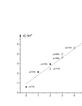
Figure 1: Our assignment of radial number $n$ to the $\rho$-mesons from Table 1. The well-established states are filled.

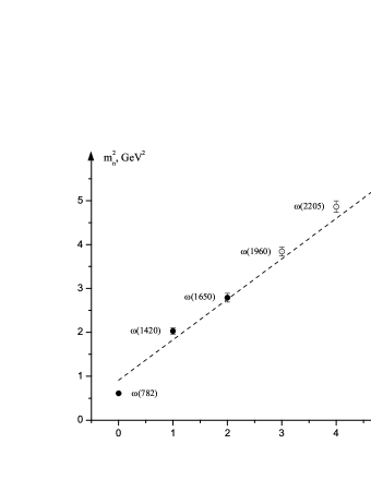
Figure 2: Our assignment of $n$ to the $\omega$-mesons from Table 1.

A more reasonable strategy for making estimates consists in the direct use of the slope which is controlled by the parameter $a$ in (11). But the accurate extraction of $a$ from the data in Table 1 is not so straightforward as it may seem. First of all, more than a half of states are not well confirmed or poorly known. The unconfirmed states have a different degree of belief. For instance, a concrete mean mass for $\rho(1900)$ is even not given in the Particle Data [7] (we have used an experimental result of Ref. [9]). The question arises whether we should use these states for fitting the linear trajectory and if we should, then which weight must be ascribed to each of these states in averaging procedure. The use of three well-established states for drawing the linear trajectory is also questionable. First of all, the ground vector states lie noticeably below the linear trajectory. This situation is common for the vector quarkonia [10]. Since we do not know reliably the underlying reason, it could make sense to exclude the ground states from the trajectory. The first radially excited states — $\rho(1450)$ and $\omega(1420)$ — are situated unnaturally higher the linear trajectory and, in fact, have a peculiar status. The matter is that they represent just names for broad resonance regions rather than well defined resonances [7]. As is emphasized in Particle Data, the mass $m_{\rho(1450)}=1465\pm 25$ MeV is ”only an educative guess”. This resonance seems to have some admixture of the strange quark (enlarging its mass) and its decays show characteristics of hybrids [7]. The situation with $\omega(1420)$ is similar. The resonances $\rho(1700)$ and $\omega(1650)$ also have much less clear status than $\rho(770)$ and $\omega(782)$. In addition, they are often interpreted as the $D$-wave vector states. In the compilations [11, 12], they give rise to the second radial vector trajectory (the first one contains the $S$-wave states). Such an interpretation is typical for semi-relativistic potential models [13]. According to this physical picture, the given states do not represent the radial excitations of $\rho$ and $\omega$. Thus, we see that all well-established vector mesons have specific problems which do not allow one to make a reliable fit.

In spite of all these uncertainties, if we look at tentative linear trajectories for various light non-strange mesons [11, 12], a remarkable feature emerges: The slope is approximately universal quantity, i.e. it weakly depends on quantum numbers of trajectory. This observation is a strong argument in favor of the hypothesis (inspired by the hadron string models [14]) that the slope is mainly determined by the gluodynamics. On the other hand, within the SW holographic model [6], the slope is also universal for mesons of any spin and parities and even for glueball trajectories. The use of the universal slope for estimates of $T_{c}$ partly resolves the problem of dependence of the predicted value for $T_{c}$ on the quantum numbers of mesons under consideration. According to the review [12], the mean slope of radial trajectories is (in terms of (11)): $4a=1.14$ GeV². Substituting this value to (9) we obtain

$$T_{c}\approx 263~{}\text{MeV}.$$ (13)

This estimate gives much larger value for $T_{c}$ than predicted by (12). The discrepancy is caused by the fact that the relation (11) yields a much heavier ”$\rho$-meson”, about 1068 MeV for the real phenomenological slope.

As follows from our discussions, if one normalizes not to the physical $\rho$-meson mass but to the best fit, the predicted $T_{c}$ is increased. A similar situation takes place in the HW model. The best global fit is achieved at the cutoff value $z_{0}=(346~{}\text{MeV})^{-1}$ [5]. This would correspond to a heavier $\rho$-meson, $m_{\rho}=832$ MeV [5], and a higher (in comparison with (10)) value for the deconfinement temperature, $T_{c}=131$ MeV.

Comparison of theoretical predictions for the deconfinement temperature with the corresponding lattice results deserves a special consideration. The lattice simulations measure $T_{c}$ in units of some dimensional quantity. The standard choice for this quantity is the string tension $\sigma$ which is obtained from the linear behavior of the potential between two static quarks at a large separation, $U(r)=\sigma r$ at large distance $r$. The standard value of $\sigma$ used in the most of lattice simulations is $\sqrt{\sigma}=420$ MeV. The prediction (12) practically coincides with the lattice result of Ref. [8]. This coincidence was the main quantitative result of Herzog’s analysis [3]. However, a closer look at the related paper [15] shows that the obtained lattice result is $T_{c}/\sqrt{\sigma}=0.419(6)$. After that a larger value for $\sigma$ was used, $\sqrt{\sigma}=460$ MeV, for predicting $T_{c}$. With the standard value of $\sigma$, the result of Ref. [15] (and of [8]) is $T_{c}\approx 175$ MeV.

In the presence of massive quarks, the deconfinement phase transition represents a crossover occurring in some range of temperatures. The exact position of this crossover depends on the observable used to define it (this is a general feature of all crossover transitions). Some time ago, the value of $T_{c}$ on the lattice with physical quarks was vastly debated in the literature. Some measurements gave the range $180-200$ MeV (e.g. [15, 16]), another measurements resulted in $150-170$ MeV (e.g. [17, 18, 19]), see Ref. [2] for a detailed discussion. But after the recent progress in extrapolating to the continuum limit and to the physical light quark masses, different lattice methods have converged to the range $150-170$ MeV [2].

This interval for $T_{c}$, however, does not suit a comparison with the estimates following from Herzog’s analysis. We wish to clearly emphasize this point. According to the philosophy of AdS/QCD correspondence, the gravitational part of the holographic action (1) is dual to pure gluodynamics in the large-$N_{c}$ limit. Hence, the predicted value for $T_{c}$ must be compared with the lattice results for gluodynamics (i.e. with non-dynamical quarks) extrapolated to large $N_{c}$. Such an extrapolation was carried out in Ref. [20]. The result is: $T_{c}/\sqrt{\sigma}=0.5949(17)+0.458(18)/N_{c}^{2}$. With $\sqrt{\sigma}=420$ MeV, this extrapolation leads to $T_{c}=250$ MeV in the large-$N_{c}$ limit. For $N_{c}=3$, one has $T_{c}=271$ MeV. This interpolation agrees with the lattice simulations for $SU(3)$ Yang–Mills theory in Refs. [21] ($T_{c}/\sqrt{\sigma}=0.629(3)$, $T_{c}=264(1)$ MeV) and [22] ($T_{c}/\sqrt{\sigma}\approx 0.65$, $T_{c}\approx 273$ MeV).

Finally we see that the prediction (13) of the SW model looks much more successful than the prediction (12) claimed in the original paper [3]. In addition, the self-consistency of the method is improved: The deconfinement phase transition is of the 1-st order in the $N_{c}\geq 3$ gluodynamics and its strength grows with $N_{c}$ [23]. This means that in the limit $N_{c}\rightarrow\infty$, the transition becomes of the same type as the Hawking–Page phase transition.

4 Deconfinement temperature in modified SW Models

4.1 The generalized SW model

The linear vector spectrum (11) of the standard SW model [6] contains a strictly fixed intercept. If we interpolate the points in Fig. 1 or 2 by the linear function, the realistic spectrum will differ from the pattern (11). Let us generalize the spectrum (11),

$$m_{n}^{2}=4a(n+1+b),\qquad n=0,1,2,\dots,$$ (14)

where the parameter $b$ will control the intercept for phenomenological spectra. The generalization of the SW model [6] which leads to the vector spectrum (14) is known [24]. It requires the following form for the dilaton profile in (1),

$$\Phi=az^{2}-2\ln{U(b,0;az^{2})},$$ (15)

here $U$ denotes the Tricomi hypergeometric function ($U(0,0;x)=1$). The deconfinement temperature will depend now not only on the slope parameter $a$ but also on the intercept parameter $b$. Below we briefly study this dependence.

The expression (8) is generalized to

$$\Delta V=\frac{1}{2}\pi\kappa L^{5}y_{h}\left[\frac{U^{2}(b,0;0)}{4y_{h}^{2}}-\int\limits_{y_{h}}^{\infty}\frac{dt}{t^{3}}U^{2}(b,0;t)e^{-t}\right]=\\ \frac{\pi\kappa L^{5}}{2z_{h}^{3}}\left\{e^{-y_{h}}U^{2}(b,0;y_{h})(y_{h}-1)+2by_{h}e^{-y_{h}}U(b,0;y_{h})U(1+b,1;y_{h})+\right.\\ \frac{1}{2\Gamma(1+b)}-y_{h}^{2}\int\limits_{y_{h}}^{\infty}\frac{dt}{t}e^{-t}\left[U^{2}(b,0;t)+4bU(1+b,1;t)U(b,0;t)+\right.\\ \left.\left.2b^{2}U^{2}(1+b,1;t)+2b(1+b)U(2+b,2;t)U(b,0;t)\right]\right\}.$$ (16)

The equation $\Delta V=0$ yields $y_{h}$ at a given $b$, after that $T_{c}$ is determined from the relation $T_{c}=(\pi\sqrt{y_{h}/a})^{-1}$. The dependence of $T_{c}/\sqrt{a}$ on $b$ in the interval $-0.5\leq b\leq 0.5$ is displayed in Fig. 3. For $b\gtrsim-0.3$, this dependence is practically linear,

$$T/\sqrt{a}=0.496+0.670b.$$ (17)

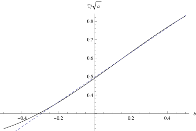
Figure 3: The dependence of $T_{c}/\sqrt{a}$ on $b$ (see text). The dotted line shows the interpolation (17).

One can fix some value of $T_{c}$ and find a parametric curve on the $(a,b)$ plane corresponding to the given $T_{c}$. For the value (13), this curve is shown in Fig. 4. The points on (or close to) this curve correspond to the choices of $a$ and $b$ at which the generalized SW model reproduces more or less the physical value of $T_{c}$ in gluodynamics. It looks really surprising that the simplest version of the SW model ($b=0$) introduced in Ref. [6] belongs to the physically acceptable region on the $(a,b)$ plane.

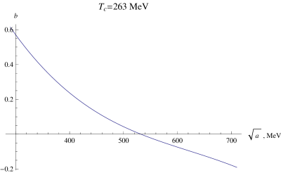
Figure 4: The parametric curve on the $(a,b)$ plane corresponding to $T_{c}=263$ MeV.

Consider, in the spirit of Ref. [3], the prediction of $T_{c}$ from a realistic vector spectrum. For this purpose, we need to extract the parameters $a$ and $b$ from the $\rho$ or $\omega$ spectrum in Table 1. As we discussed in Sect. 3, the extracted values will strongly depend on the choice of data and on the weight of each state in the fit. In this situation, the account for the experimental errors in the mass determination is not very informative since, in practice, such errors are subleading in the final fit. We will take the central values of the masses and the predicted $T_{c}$ should be regarded as an estimate. We analyze how different hypotheses on the choice of data for interpolating the linear trajectory influence on the predicted value of $T_{c}$. The results are summarized in Table 2.

Some comments are in order. We considered three hypotheses. In the first one, only the well-established states are used. In this case, the predicted value of $T_{c}$ lies a bit below the interval $150-170$ MeV given by lattices with dynamical light quarks and the $\rho$ and $\omega$ sectors yield close results. Next we add the poorly known states except the following resonances: the $n=5$ excitations as the least established states, the $\rho(1570)$ and $\rho(1900)$ since they represent $\phi\pi$ states with a large hidden strange component appearing jointly in a certain fit of experimental data [9]. Here the $\rho$ and $\omega$ sectors result in quite different predictions. Most likely, this is related with an insufficient accuracy of the experimental data. A definite choice for the $\rho$ and $\omega$ states leads to a prediction of $T_{c}$ in the interval $250-270$ MeV expected in gluodynamics. This choice constitutes our third hypothesis. Such a possibility is interesting because the requirement of a correct reproduction of $T_{c}$ could serve as a guide for the prediction (confirmation) of new resonances within the SW model.

Table 2: Some predictions for $T_{c}$ basing on Table 1, Figs. 1 and 2, relations (14) and (16) (see text).

Particle	Radial states	$m_{n}^{2}$, GeV2	$T_{c}$, MeV
$\rho$	$n=0,1,2$	$1.18(n+0.61)$	$143$
$\omega$	$n=0,1,2$	$1.09(n+0.66)$	$149$
$\rho$	$n=0,1,2,3,4$	$0.99(n+0.89)$	$207$
$\omega$	$n=0,1,2,3,4$	$1.03(n+0.74)$	$166$
$\rho$	$n=0,1,2,4,5$	$0.88(n+1.12)$	$270$
$\omega$	$n=1,2,3,4$	$0.95(n+1.04)$	$255$

4.2 The SW model with the UV cutoff

The linear radial Regge trajectory is only an approximation to the observable spectrum. The attempts to introduce non-linearities into the SW model lead usually to models admitting only numerical treatment. We will consider the model of Ref. [25] which can be solved analytically. The non-linearity of the SW spectrum is introduced in [25] via imposing the ultraviolet (UV) cutoff. An heuristic physical motivation is rather simple. In the UV regime, QCD represents a weakly coupled gauge theory, hence, according to the ideas of holographic duality, its probable holographic dual should be in the strong coupling regime. This makes questionable the applicability of a semiclassical approximation to the dual theory when $z\rightarrow 0$. The introduction of UV cutoff is a crude way for avoiding this problem. The vector spectrum becomes non-linear, it is given by zeros of the Tricomi function $U(-m_{n}^{2}/(4a),0;aL^{2})$ [25], where $L$ is the AdS radius and the cutoff is imposed (without loss of generality) at $z_{UV}=L$. The spectrum has the form $m_{n}^{2}=4af_{n}(aL^{2})$ with $f_{n}$ representing a function of the cutoff value. For example, $f_{n}(1)=\{1.57,2.84,4.05,5.22,6.37,\dots\}$.

The comparison of the model with the real spectra was not performed in Ref. [25]. For our purposes, we partly analyze the ensuing phenomenology. It is convenient to rewrite the spectrum (11) in units of the ground mass,

$$m_{n}^{2}=m_{0}^{2}\{1,2,3,\dots\}.$$ (18)

In these notations, the $\rho$ and $\omega$ spectra from Table 1 are

$$m_{\rho,n}^{2}=m_{\rho}^{2}\{1,3.6,4.9,?,7.7,8.5\},\quad m_{\omega,n}^{2}=m_{\omega}^{2}\{1,3.3,4.5,6.3,7.9,?\}.$$ (19)

The non-zero cutoff does not allow to improve the agreement of (18) with the experimental patterns (19). However, consider the axial-vector $a_{1}$-mesons. The Particle Data [7] cites one well-established resonance of the mass $1230\pm 40$ MeV and three poorly known states with the masses $1647\pm 22$, $1930^{+30}_{-70}$, and $2270^{+55}_{-40}$ MeV. The spectrum can be written as

$$m_{a_{1},n}^{2}=m_{a_{1}}^{2}\{1,1.8,2.5,3.4\}.$$ (20)

The model prediction in the example above is

$$aL^{2}=1:\qquad m_{n}^{2}=m_{0}^{2}\{1,1.8,2.6,3.3,4.1,\dots\}.$$ (21)

We see that the spectra (20) and (21) are very close, i.e. the SW model with the UV cutoff is able to provide an accurate description for the axial-vector spectrum. This supports the arguments of Ref. [25] that the UV cutoff mimics the chiral symmetry breaking.

We will use this property of the model under consideration to estimate $T_{c}$ from the axial-vector sector. The extension of (8) to the case of finite UV cutoff $z=\epsilon$ is

$$\Delta V=\frac{1}{2}\pi\kappa L^{5}z_{h}\left[\int\limits_{y_{\epsilon}}^{y_{h}}\frac{dt}{t^{3}}e^{-t}-\sqrt{1-\frac{y_{\epsilon}^{2}}{y_{h}^{2}}}\int\limits_{y_{\epsilon}}^{\infty}\frac{dt}{t^{3}}e^{-t}\right],$$ (22)

where $y_{h}\equiv az_{h}^{2}$, $y_{\epsilon}\equiv a\epsilon^{2}$. The equation $\Delta V=0$ allows one to find $y_{h}$ from a fixed value of $y_{\epsilon}$. Taking the fit considered above, $y_{\epsilon}=1$, we obtain numerically $y_{h}\approx 1.40$ that for the mean value of the radial slope, $4a=1.14$ GeV², corresponds to $T_{c}\approx 144$ MeV. This prediction practically coincides with that of the $\rho$-meson sector in Table 2.

5 Discussions

The contribution of the chiral symmetry breaking to the full holographic action scales as $N_{c}$. Since the prediction of $T_{c}$ comes from the gluonic part (1) scaling as $N_{c}^{2}$, one could naively think that the axial-vector spectrum is equally good for predicting $T_{c}$ and estimate a discrepancy with the vector case at the $1/N_{c}$ level. This expectation is of course not correct. Even the rough analysis of Ref. [3] would give a unrealistically large difference $T_{c}^{(a_{1})}/T_{c}^{(\rho)}=m_{a_{1}}^{2}/m_{\rho}^{2}\approx 2.5$. For a more consistent prediction we should extract the parameters $a$ and $b$ from the linear fit of the $a_{1}$ trajectory and find $T_{c}$ from the generalized SW model. The result is $a\approx 0.30$ GeV², $b\approx 0.25$ which leads to $T_{c}\approx 363$ MeV. The large enhancement of predicted $T_{c}$ occurs due to a large value of $b$ — this is clear from Fig. 3 and the approximate relation (17). The prediction for the deconfinement temperature from the axial-vector sector is surprisingly close to the estimates from the vector one if the SW model with the UV cutoff is exploited.

Since the results of lattice simulations are usually given in units of the string tension $\sigma$, the possible errors in determination of $\sigma$ entail some uncertainty in the lattice predictions for $T_{c}$. This source of uncertainty could be avoided if theoretical predictions were also expressed in terms of $T_{c}/\sqrt{\sigma}$. Unfortunately, such an expression is model dependent. For instance, if we assume the string (flux tube) picture of mesons, assume that the meson string is of the Nambu–Goto type and identify the tension of relativistic string with the tension of non-relativistic linear potential, then the slope (11) is given by [26, 27]

$$4a=2\pi\sigma,$$ (23)

i.e. $\sqrt{a}=\sqrt{\pi/2}\sqrt{\sigma}\approx 1.25\sqrt{\sigma}$ in (9) and in similar formulas. In particular, the result (9) becomes $T_{c}/\sqrt{\sigma}\approx 0.62$ which agrees well with the lattice predictions (see Sect. 3). The phenomenological mean slope [12] 1.14 GeV² yields $\sqrt{\sigma}\approx 426$ MeV if we use (23). This value is also close to many lattice measurements, $\sqrt{\sigma}\approx 420$ MeV. The assumptions above lead thus to a reasonable picture. We give an heuristic derivation of the slope (23) in the appendix.

The requirement of the existence of a non-zero deconfinement temperature restricts the possible form for the dilaton background $\Phi$ in the holographic action (1). It is easy to check that if the sign of $\Phi$ is changed then $\Delta V<0$ in (8) at all temperatures, i.e. the model is always in the deconfined phase. This conclusion seems to contradict to the Sonnenschein criterion of confinement  [28] based on the Wilson loop area law for the confinement of strings. According to this criterion, the time–time metric component $g_{00}$ should satisfy the conditions

$$\partial_{z}(g_{00})|_{z=z_{0}}=0,\qquad g_{00}|_{z=z_{0}}\neq 0.$$ (24)

The AdS metric (2) does not satisfy (24). The dilaton profile $e^{-\Phi}$, however, can be rewritten as a part of the metric which becomes asymptotically ($z\rightarrow 0$) AdS. The choice $\Phi=az^{2}$ results in monotonically decreasing $g_{00}$, the condition (24) cannot be fulfilled, while the choice $\Phi=-az^{2}$ provides a non-trivial minimum for $g_{00}$ matching the confinement criterion (24). This property was exploited in Ref. [29] for a derivation of the linear confinement potential from the holographic approach and later triggered an active use of the SW models with inverse dilaton profile (see, e.g., [30, 31]) in spite of a formal existence of massless vector mode [32]. Thus we see that the black hole and Wilson loop criteria for confinement are in conflict in the simplest version of the SW model. A resolution of this puzzle would be interesting. An obvious possibility consists in a modification of the dilaton profile $e^{-az^{2}}$ with preserving its infrared asymptotics.

In the gravitational action (1), the form of the dilaton background is the same as in the SW model of Ref. [6]. It should be noted that in reality this represents a rather strong assumption as long as the SW model has not been derived from any string theory. One can simply imagine a situation when this assumption is violated. Indeed, suppose that the planar gluodynamics is dual to the closed string sector of a full dual theory. Then constructing an effective gravity dual in AdS_d space one commonly arrives at the expression

$$I=\int d^{d}xe^{-2\Phi}\sqrt{g}L_{\text{grav}}+\int d^{d}xe^{-\Phi}\sqrt{g}L_{\text{matter}},$$ (25)

in which the condensate $\Phi$ of a massless scalar field (called the dilaton) controls the string coupling. In realistic models of physics, the gravitational part of (25) may contain a dilaton potential possessing some minimum, say at $\Phi=az^{2}$. Comparing (25) with (1) we should then conclude that the dilaton contribution is rescaled by the factor of 2 in the gluonic part in comparison with the mesonic part of the action. This means that the slope parameter should be rescaled as $a\rightarrow 2a$ in making predictions for $T_{c}$. The prediction (9) becomes $T_{c}\approx 0.49\sqrt{2a}\approx 0.70\sqrt{a}$ yielding $T_{c}\approx 372$ MeV instead of (9). Note that if we use the fit of the original analysis [3], where $m_{\rho}^{2}$ is identified with the slope, the prediction (12) is $T_{c}\approx 0.348m_{\rho}=270$ MeV, which lies amusingly close to the lattice predictions in the $SU(3)$ Yang–Mills theory [21, 22]. This agreement hints at the idea that a SW-like model leading to the vector spectrum $m_{n}^{2}=4a(n+1/2)$ would be successful in predicting $T_{c}$ on the base of (25). Using some modifications of the holographic prescriptions, such a variant of the SW model was proposed in Ref. [31]. Its spectrum reads $m^{2}=4a(n+(L+J)/2)$, where $J$ is the total spin and $L$ denotes the orbital momentum of a quark–antiquark pair. Here the vector spectrum ($L=0$, $J=1$) is degenerate with the scalar one ($L=1$, $J=0$) and is automatically shifted with respect to the axial-vector spectrum ($L=1$, $J=1$).

In the case of free intercept, the relation (25) suggests to rescale the dilaton (15),

$$\Phi=2az^{2}-4\ln{U(b,0;az^{2})},$$ (26)

that renders (16) into

$$\Delta V=\frac{1}{2}\pi\kappa L^{5}y_{h}\left[\frac{U^{4}(b,0;0)}{4y_{h}^{2}}-\int\limits_{y_{h}}^{\infty}\frac{dt}{t^{3}}U^{4}(b,0;y)e^{-2y}\right].$$ (27)

The condition $\Delta V=0$ gives now another predictions for $T_{c}$. For the input data in Table 2, these predictions are shown in Table 3.

Table 3: The predictions for the deconfinement temperature based on inputs from Table 2 in the case of replacement (16) by (27).

Particle	Radial states	$m_{n}^{2}$, GeV2	$T_{c}$, MeV
$\rho$	$n=0,1,2$	$1.18(n+0.61)$	$159$
$\omega$	$n=0,1,2$	$1.09(n+0.66)$	$170$
$\rho$	$n=0,1,2,3,4$	$0.99(n+0.89)$	$299$
$\omega$	$n=0,1,2,3,4$	$1.03(n+0.74)$	$199$
$\rho$	$n=0,1,2,4,5$	$0.88(n+1.12)$	$400$
$\omega$	$n=1,2,3,4$	$0.95(n+1.04)$	$381$

Finally we see that predictions for the deconfinement temperature depend strongly on assumptions as regards the possible origin of the SW model from a dual string theory.

6 Conclusions

We have analyzed in detail various aspects of the prediction for the deconfinement temperature $T_{c}$ from the bottom–up holographic models of QCD. It was argued that the predicted $T_{c}$ must refer to deconfinement phase transition in the pure gluodynamics. The agreement of the prediction of the simplest soft wall model [6] with the recent lattice results looks impressive. We have also shown that if the soft wall model is accommodated for a description of realistic vector spectra, the predicted $T_{c}$ becomes ambiguous because of lack of sufficient amount of reliable experimental data on the radially excited light mesons. The use of well-established states results in $T_{c}$ close to the crossover transition in the lattice simulations with dynamical quarks.

The arising relations between parameters of the observed radial trajectories of light mesons and the deconfinement temperature in the planar QCD represent a curious theoretical result of the holographic approach. The fact that in many cases these relations agree well with the lattice results means that the holographic trick seems to pass an important phenomenological test. On the other hand, the requirement of a reasonable prediction for $T_{c}$ can serve as a strong restriction on the possible variants of the holographic models. These restrictions may be useful for predicting new resonances.

Appendix

There exists a simple heuristic way for the derivation of the linear radial trajectory from the semiclassical flux tube model for the light mesons [34]. It leads to the wrong slope; nevertheless, it is occasionally used in the literature and in discussions. We briefly reproduce this derivation and then correct it.

Consider a thin gluon flux tube of length $r$ stretched between massless quark and antiquark. The energy of the system (the meson mass) is

$$M=2\sqrt{p}+\sigma r,$$

where $p$ denotes the momentum of quarks oscillating in the linear confinement potential. The tension of the flux tube (the string tension) is defined by $\sigma=M/l$, here $l$ means the maximal quark separation. Impose the Bohr–Sommerfeld quantization condition on the quark momentum,

$$\int\limits_{0}^{l}pdr=\pi(n+b),\qquad n=0,1,2,\dots.$$

The constant $b$ depends on the boundary conditions ($b=1/2$ for the centrosymmetrical potentials). A trivial integration results in the relation

$$M^{2}=4\pi\sigma(n+b).$$

The slope obtained is twice the slope of the Nambu–Goto string (23). The source of the discrepancy lies in the unphysical assumption as regards the massless quarks which, was used in the essentially non-relativistic derivation.

Let us introduce the quark masses $m_{1}$ and $m_{2}$ and consider the system in the rest frame of the quark 1. The energy of the system is

$$M=m_{1}+\sqrt{p^{2}+m_{2}^{2}}+\sigma r.$$

Assume that $m_{2}$ is much less than the typical momentum $p$, $m_{2}^{2}/p^{2}\ll 1$. Repeating the derivation above, we get

$$(M-m_{1})^{2}\simeq 2\pi\sigma(n+b).$$

Insofar as $m_{1},m_{2}\ll M$ in the light mesons, we can safely neglect the small mass contributions stemming from $m_{1}$ and $m_{2}$. The final Regge-like formula has the correct slope.

References

- [1] A. V. Smilga, Phys. Rept. 291, 1 (1997) [hep-ph/9612347].
- [2] S. Borsanyi et al. [Wuppertal-Budapest Collaboration], JHEP 1009, 073 (2010) [arXiv:1005.3508 [hep-lat]].
- [3] C. P. Herzog, Phys. Rev. Lett. 98, 091601 (2007) [hep-th/0608151].
- [4] E. Witten, Adv. Theor. Math. Phys. 2, 505 (1998) [hep-th/9803131].
- [5] J. Erlich, E. Katz, D. T. Son and M. A. Stephanov, Phys. Rev. Lett. 95, 261602 (2005) [hep-ph/0501128]; L. Da Rold and A. Pomarol, Nucl. Phys. B 721, 79 (2005) [hep-ph/0501218].
- [6] A. Karch, E. Katz, D. T. Son and M. A. Stephanov, Phys. Rev. D 74, 015005 (2006) [hep-ph/0602229].
- [7] J. Beringer et al. (Particle Data Group), Phys. Rev. D 86, 010001 (2012).
- [8] F. Karsch, J. Phys. Conf. Ser. 46, 122 (2006) [hep-lat/0608003].
- [9] B. Aubert et al. [BaBar Collaboration], Phys. Rev. D 77, 092002 (2008) [arXiv:0710.4451 [hep-ex]].
- [10] S. S. Afonin and I. V. Pusenkov, arXiv:1308.6540 [hep-ph].
- [11] A. V. Anisovich, V. V. Anisovich and A. V. Sarantsev, Phys. Rev. D 62, 051502(R) (2000).
- [12] D. V. Bugg, Phys. Rept. 397, 257 (2004).
- [13] S. Godfrey and J. Napolitano, Rev. Mod. Phys. 71, 1411 (1999).
- [14] Y. Nambu, Phys. Rev. D 10, 4262 (1974).
- [15] M. Cheng, N. H. Christ, S. Datta, J. van der Heide, C. Jung, F. Karsch, O. Kaczmarek and E. Laermann et al., Phys. Rev. D 74, 054507 (2006) [hep-lat/0608013].
- [16] A. Bazavov, T. Bhattacharya, M. Cheng, N. H. Christ, C. DeTar, S. Ejiri, S. Gottlieb and R. Gupta et al., Phys. Rev. D 80, 014504 (2009) [arXiv:0903.4379 [hep-lat]].
- [17] Y. Aoki, Z. Fodor, S. D. Katz and K. K. Szabo, Phys. Lett. B 643, 46 (2006) [hep-lat/0609068].
- [18] A. Bazavov, T. Bhattacharya, M. Cheng, C. DeTar, H. T. Ding, S. Gottlieb, R. Gupta and P. Hegde et al., Phys. Rev. D 85, 054503 (2012) [arXiv:1111.1710 [hep-lat]].
- [19] C. Bernard et al. [MILC Collaboration], Phys. Rev. D 71, 034504 (2005) [hep-lat/0405029].
- [20] B. Lucini, A. Rago and E. Rinaldi, Phys. Lett. B 712, 279 (2012) [arXiv:1202.6684 [hep-lat]].
- [21] G. Boyd, J. Engels, F. Karsch, E. Laermann, C. Legeland, M. Lutgemeier and B. Petersson, Nucl. Phys. B 469, 419 (1996) [hep-lat/9602007].
- [22] Y. Iwasaki, K. Kanaya, T. Kaneko and T. Yoshie, Nucl. Phys. Proc. Suppl. 53, 429 (1997) [hep-lat/9608090].
- [23] B. Lucini and M. Panero, Prog. Part. Nucl. Phys. 75, 1 (2014) [arXiv:1309.3638 [hep-th]].
- [24] S. S. Afonin, Phys. Lett. B 719, 399 (2013) [arXiv:1210.5210 [hep-ph]].
- [25] S. S. Afonin, Phys. Rev. C 83, 048202 (2011) [arXiv:1102.0156 [hep-ph]].
- [26] B. Zwiebach, A First Course in String Theory (Cambridge University Press, Cambridge, 2004).
- [27] M. Baker and R. Steinke, Phys. Rev. D 65, 094042 (2002).
- [28] J. Sonnenschein, hep-th/0009146.
- [29] O. Andreev and V. I. Zakharov, Phys. Rev. D 74, 025023 (2006) [hep-ph/0604204].
- [30] F. Zuo, Phys. Rev. D 82, 086011 (2010) [arXiv:0909.4240 [hep-ph]]. S. S. Afonin, Int. J. Mod. Phys. A 27, 1250171 (2012); 25, 5683 (2010). G. F. de Teramond and S. J. Brodsky, Nucl. Phys. Proc. Suppl. 199, 89 (2010) [arXiv:0909.3900 [hep-ph]]. G. F. de Teramond, H. G. Dosch and S. J. Brodsky, Phys. Rev. D 87, no. 7, 075005 (2013) [arXiv:1301.1651 [hep-ph]].
- [31] T. Branz, T. Gutsche, V. E. Lyubovitskij, I. Schmidt and A. Vega, Phys. Rev. D 82, 074022 (2010) [arXiv:1008.0268 [hep-ph]].
- [32] A. Karch, E. Katz, D. T. Son and M. A. Stephanov, JHEP 1104, 066 (2011) [arXiv:1012.4813 [hep-ph]].
- [33] M. Ademollo, G. Veneziano and S. Weinberg, Phys. Rev. Lett. 22, 83 (1969).
- [34] M. Shifman, hep-ph/0507246.