The Three Discrete Nulling Timescales of PSR J1717$-$4054

Abstract

PSR J1717$-$4054 is one of the small class of pulsars which null on intermediate ($\sim$hour) timescales. Such pulsars represent an important link between classical nullers—whose emission vanishes for a few rotations—and the intermittent pulsars which null for months and years. Using the Parkes radio telescope and the Australia Telescope Compact Array, we have studied the emission from PSR J1717$-$4054 over intervals from single pulses to years. We have identified and characterised nulling at three discrete timescales: the pulsar emits during “active states” separated by nulls lasting many thousands of rotations, while active states themselves are interrupted by nulls with a bimodal distribution of durations—one to two rotations, or tens of rotations. We detect no subpulse structure or flux density variations during active states, and we place stringent limits ($<0.1$% of the mean active flux density) on pulsed emission during inactive states. Finally, our high-quality data have also allowed us to measure for the first time many important properties of PSR J1717$-$4054, including its position, spindown rate, spectrum, polarization characteristics, and pulse broadening in the interstellar medium.

1 Introduction

Nulling pulsars, first identified by Backer (1970b), spontaneously and suddenly (typically within one rotation) cease to emit at a detectable level. After an interval ranging from a few rotations (e.g. Wang, Manchester & Johnston, 2007) to a few years, e.g. PSR J1841$-$0500 ($\sim$600 days, Camilo et al., 2012), emission resumes just as suddenly. This wide range of timescales, most of which are significantly longer than those natural to a pulsar magnetosphere, is difficult to explain through a single mechanism.

Because radio emission arises from coherent plasma processes, short nulls have been interpreted as fluctuations in the plasma state that briefly disrupt or alter the required coherency. In other pulsars—particularly those with drifting subpulses—the nulling phenomenon may be related to the geometry of a drifting “carousel” of sparks (Deshpande & Rankin, 1999; Rankin & Wright, 2008) whose drift rate depends on the local charge density above the polar cap. For example, Unwin et al. (1978) determined the subpulse drift rate of PSR B0809+74 drops to zero during nulls, while Herfindal & Rankin (2007) identified subpulse periodicity persisting through nulls in PSR B1133$+$16, suggesting these short nulls are simply gaps in the drifting beam pattern.

On the other hand, the pulsars that null on long timescales, e.g. PSR B1931$+$24 ($\sim$30 days, Kramer et al., 2006), PSR J1841$-$0500 ($\sim$600 days, Camilo et al., 2012), and PSR J1832$+$0029 ($\sim$600–800 days, Lorimer et al., 2012) are intermittent in the sense that the currents and particle acceleration powering radio emission may cease, or at the very least change sufficiently to steer the radio beam away from the earth (e.g. Timokhin, 2010). The key piece of evidence comes from the measurement of the spindown rate ($\dot{\nu}$) of each state, which decreases by a factor of 1.5–2.5 when the pulsar is nulling, indicating a dramatic reconfiguration of the magnetospheric currents and, consequently, torque.

Similar switches between metastable magnetosphere/spindown states have been identified by Lyne et al. (2010), who discovered a quasiperiodic modulation of the spindown rate in a sample of pulsars monitored over several decades. Moreover, they found that in some pulsars, switches between $\dot{\nu}$ levels were accompanied by changes in pulse profile (i.e. mode changes, Backer, 1970a), thus linking emission properties to magnetosphere state. The stochastic switches between $\dot{\nu}$ states introduce red noise into timing residuals relative to a spindown model with a single $\dot{\nu}$, suggesting that such state switching may be of fundamental importance to the timing noise phenomenon and thus to pulsar timing arrays.

These long timescale observations make abundantly clear that at least some pulsars switch between metastable magnetospheres. However, because switches happen rarely and rapidly, it is difficult to catch these pulsars “in the act” and gain insight into both what these states physically represent and how the switching is accomplished. Pulsars with intermittency of hours likely also represent magnetospheric switching, though the intermittent durations are too short to measure independent values of $\dot{\nu}$. Such pulsars can be targeted with observations to resolve all relevant timescales and may thus yield clues to the switching process. In a clear example of the power of such systems, Hermsen et al. (2013) discovered that the X-ray emission from PSR B0943$+$10 is correlated with radio mode changes, implying rapid cooling of the neutron star polar cap after the pulsar switches from its radio-faint to its radio-bright mode.

PSR J1717$-$4054, discovered by Johnston et al. (1992) in a 20 cm Parkes survey of the Galactic plane, is a strong nuller and is inactive most of the time. Indeed, in a 2-hr observation, Wang, Manchester & Johnston (2007) observed only one brief, 3.5 minute burst of emission, leading those authors to conclude the nulling fraction is $>$95%. During these scarce active states, the pulsar continues to null, albeit at a much lower rate. Hereafter, to distinguish between the multi-hour nulls separating active periods (APs) and the $<$1-minute nulls within active periods (see below), we refer to long nulls as inactive periods (IPs).

With the lengthy breaks between APs, the telescope time required to obtain many realizations of this cycle is prohibitive. Instead, in order to monitor the long-term behaviour of PSR J1717$-$4054, we used short, low time-resolution snapshot observations obtained over six years with the Parkes radio telescope. To access short timescales, we complemented these with two rise-to-set Parkes observations of 9.5 hr during which we obtained high time-resolution data. During the first track, we also observed PSR J1717$-$4054 simultaneously with the Australia Telescope Compact Array (ATCA). With these data, we have characterised the intermittency timescale and identified nulling at two discrete timescales within APs; we have also measured for the first time many important properties of PSR J1717$-$4054.

In §2, we describe our monitoring observations and discuss the resulting long-term timing solution, study of flux stability, and measurement of typical AP/IP duration. In §3, we describe our long-track Parkes and ATCA observations, and we present in detail the emission properties of the pulsar within its active periods. We additionally use these well-calibrated data to measure the polarization and pulse broadening of PSR J1717$-$4054 and to place a stringent limit on any persistent emission from IPs. We present a likelihood-based method for identifying pulse nulls and present the resulting analysis of nulling within APs. Finally, we summarise and interpret our results in §4.

2 Monitoring Observations and Long-timescale Properties

Table 1: Measured and Derived Parameters for PSR J1717$-$4054

Parameter	Value
Right ascension, R.A. (J2000.0)	$17\mathrm{{}^{h}}17\mathrm{{}^{m}}$52$\aas@@fstack{s}$22(7)
Declination, decl. (J2000)	–41°03′17″(4)
Position epoch (MJD)	56671
Frequency, $\nu$ (Hz)	1.1264838005(3)
Frequency derivative, $\dot{\nu}$ ($10^{-15}$ Hz/s)	–4.661(1)
Frequency epoch (MJD)	53200
Characteristic age, $\tau_{c}$ (Myr)	3.8
Spindown luminosity, $\dot{\mathrm{E}}$ (erg s-1)	$2.1\times 10^{32}$
Dipole magnetic field, B ($10^{12}$ G)	1.8
DM Distance (NE2001, kpc)	4.7
Flux density, 732 MHz (mJy)	17(1)
Flux density, 1369 MHz (mJy)	5.2(2)
Flux density, 3094 MHz (mJy)	1.0(1)
Flux density, 1400  MHz, S1400 (mJy)	4.9
Spectral index, $\alpha$	–1.9(1)
Dispersion measure, DM (pc cm-3)	306.9(1)
Rotation measure, RM (rad m-2)	–800(100)
Scattering timescale, $\tau_{sc,732}$ (ms)	60(6)
Scattering timescale, $\tau_{sc,1369}$ (ms)	7(1)
Scattering timescale $\tau_{sc,1000}$ (ms)	20
Inactive fraction (%)	80(15)
Active nulling fraction (%)	6.8(3)
Mean active state (AP) duration (s)	1100(180)
Mean inactive state (IP) duration (s)	4300(800)

Note. — Numbers in parentheses give the uncertainty on the terminal significant figure(s). The formal uncertainties on flux densities and timescales are smaller than systematic uncertainties, which we estimate to be about 10%.

2.1 Observations

The PULSE@Parkes program (Hollow et al., 2008) provides high school students the opportunity to remotely control and observe pulsars with the 64m Parkes radio telescope, and the data obtained are used for both educational and scientific purposes (Hobbs et al., 2009). During two-hour observing sessions, students work in small groups and select suitable pulsars from the program catalogue, observing each pulsar for a few minutes. As the project has been running since December 2007, the data set provides an excellent set of snapshot observations for a number of pulsars. Because its intermittent nature engages student interest, PSR J1717$-$4054 is typically observed in any session it is visible, resulting in 85 observations as of April 2014.

PULSE@Parkes observations are largely undertaken with the 20 cm multibeam receiver (Staveley-Smith et al., 1996), with 30 s sub-integrations of 256 MHz of bandwidth centred about 1369 MHz recorded in 1024 frequency channels and 1024 phase bins by the Parkes Digital Filterbank Mark 3 (PDFB3) or PDFB4, a nearly identical system. Each pulsar observation is preceded by observation of a cycled, coupled noise diode, allowing good polarization calibration via measurement of differential gain and phase.

We primarily processed the data using the PSRCHIVE software suite (Hotan, van Straten & Manchester, 2004). We mitigated aliased signals and narrowband RFI by, respectively, excising channels within 5% of the band edge and those with a level substantially above a median-smoothed bandpass. To convert the observed intensity to absolute flux density, we made use of observations of the radio galaxy 3C 218 (Hydra A; Baars et al., 1977) taken every few weeks to support the Parkes Pulsar Timing Array project (Manchester et al., 2013) to determine the system equivalent flux density of the calibration noise source and consequently an absolute flux scale for each Stokes parameter.

All data recorded through the PULSE@Parkes program become public immediately and are available through the CSIRO Data Archive Portal (Hobbs et al., 2011). Data taken under other programs, including those described below, are generally available after an 18-month proprietary period.

2.2 Timing Solution

Combining these data with archival observations, we used the Tempo2 software package (Hobbs, Edwards & Manchester, 2006) to obtain a phase-connected timing solution extending over six years. The residuals to a simple fit for the frequency ($\nu$) and its derivative ($\dot{\nu}$) show modest timing noise and appear in Figure 1. This is the first published measurement of $\dot{\nu}$, from which several important properties, listed in Table 1, can be estimated.

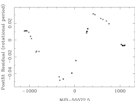
Figure 1: Residuals of 20 cm pulse times of arrival in fractions of a neutron star rotation for the best-fit timing model.

2.3 Pulsar Profile and Flux Density Variations

To measure the active-state flux density, we selected only observations in which emission was detected, and we further deleted sub-integrations visibly affected by substantial nulling or a state switch. We employed two methods of calculating the flux density: (1) simply adding up signal in excess of baseline and (2) fitting an analytic template to the profile and inferring the flux from the template scale.

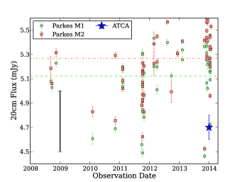
Figure 2: The absolute flux density of PSR J1717$-$4054 at 20 cm. The green circles and dashed line (mean) indicate flux densities derived using Method 1, while the salmon squares and dot-dashed line (mean) indicate flux densities derived with Method 2, i.e. by fitting a template. An uncertainty of 10%—a typical level encapsulating calibration errors and interstellar scintillation—is indicated by the black error flag in the lower lefthand corner. The blue star indicates the ATCA-derived pulsed flux density (§3.1.2).

The results, shown in Figure 2, indicate the intrinsic flux density is stable over the years of observation, with variations readily explained by modest scintillation in the interstellar medium and small calibration errors. Moreover, the flux density is mututally consistent between the two methods; since the second measurement explicitly measures flux density with the expected pulse shape while the first method measures any flux density above baseline, the pulse profile must also be stable at this level.

The mean flux density is 5.2$\pm$0.3 mJy, which is substantially different from previous values reported in the literature. Johnston et al. (1992) found 1.0 mJy from the discovery observation, but this computation did not select only APs, and is consistent with scaling our value by the inactive fraction. Hobbs et al. (2004) give a flux density of 54 mJy based on data from the Parkes multibeam pulsar survey. Because the survey pointings were substantially offset from the position of PSR J1717$-$4054, this discrepancy may have resulted from either an inaccurate model of the sensitivity at the edges of the beam or the use of an inaccurate pulsar position.

We also obtained calibrated flux measurements from the 10 cm and 50 cm observations discussed below, with flux densities of 0.96 mJy and 16.9 mJy, respectively, following a fairly typical power law $S_{\nu}=S_{0}(\nu/\nu_{0})^{\alpha}$ with $\alpha=-1.9$.

2.4 Active/Inactive Duty Cycle

With many observations of PSR J1717$-$4054, we are in a position to refine the nulling fraction (inactive fraction, in our parlance) estimate of Wang, Manchester & Johnston (2007). However, the typical time PSR J1717$-$4054 spends in either state is substantially longer than the few-minute PULSE@Parkes observations. Further, as there is a natural bias among both high schools students and astronomers to extend (curtail) observations of the pulsar when it is active (inactive), a simple tally of the total time the pulsar is observed to be bright is biased.

On the other hand, switches are random, and, if the process is memoryless (Poisson), switch rates are unaffected by observational bias. Moreover, since switches are rare for this pulsar, we expect to see no more than one state switch in a given sub-integration. Thus, to estimate switch rates from our fold-mode data, which has typical time resolution of 30 s, we classify by inspection each sub-integration into one of four classes: $IP\rightarrow AP$, $IP\rightarrow IP$, $AP\rightarrow AP$, or $AP\rightarrow IP$. We then simply count the instances of each class and tally the total time spent in each state in Table 2. Averaged over all PULSE@Parkes and archival observations, we find a rate of $IP\rightarrow AP$ of $(2.3\pm 0.4)\times 10^{-4}$ Hz and $AP\rightarrow IP$ of $(9.3\pm 1.6)\times 10^{-4}$ Hz. That is, the typical time the pulsar spends in the active (inactive) state is $1100\pm 180$ s ($4300\pm 800$ s), and the inactive fraction is $80\pm 15$%. Although limited by the small number of observed switches, we note that these rates appear to be consistent from year to year. We also note that the nulling fraction obtained by simply tallying time in each state is 77%, lower than, but consistent with, the estimate from switch counting.

Table 2: State switches from active to inactive and vice versa observed, as well as total time recorded in each state, in PULSE@Parkes and archival data.

Year	IP$\rightarrow$AP	AP$\rightarrow$IP	IP	AP	AP Frac
			(s)	(s)	(%)
2004	8	9	52584	14626	22
2005	3	3	15948	3904	20
2006	0	1	3682	1374	27
2007	2	5	14095	3757	21
2008	4	3	7326	3494	32
2009	0	0	2544	0	0
2010	2	2	2819	1193	30
2011	5	10	8159	5383	40
2012	3	2	15331	1994	11
2013	3	1	6252	2944	32
All	30	36	128740	38658	23

3 Single-pulse Observations and Short-timescale Properties

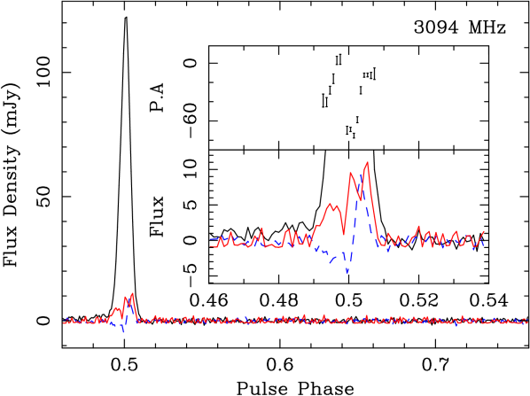
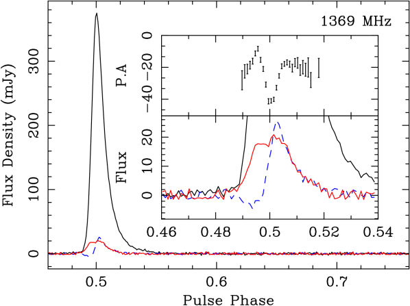
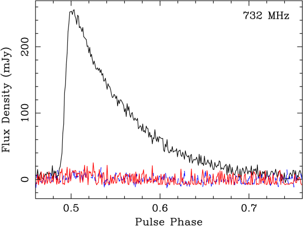
Figure 3: Pulse profiles at (top to bottom) 10 cm, 20 cm, and 50 cm. Total intensity (Stokes I) is the dominant black trace. A small amount of circular polarization (Stokes V) appears in dashed blue at 10 cm and 20 cm, as does a similar level of linear polarization (solid red). The inset in the top panel shows a zoomed view of the profile, in which appears a hint of a leading component.

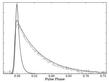
Figure 4: Stokes I profiles at 20 cm (grey, sharp) and 50 cm (grey, long tailed) along with models of the scattered profile (black) as described in the text. The scale is arbitrary.

3.1 Observations

3.1.1 Parkes

To resolve state switches and record the entirety of a series of APs and IPs, we obtained high-time-resolution observations (Parkes program P850) of PSR J1717$-$4054 during two 9.5 hr rise-to-set tracks on 13 (Day 1) and 14 (Day 2) January, 2014. On Day 1, we observed at 20 cm with the same receiver configuration described above. With PDFB4 in “search mode”, we recorded a 2-bit, 256-channel filterbank every 256 $\mu$s, while simultaneously we obtained fold-mode data with PDFB3. To maintain polarization calibration, we activated the pulsed noise source roughly every hour.

On Day 2, we collected data using an identical search-mode configuration but with a dual-band 10 cm/50 cm receiver (Granet et al., 2005), offering 1024 MHz of bandwidth at a centre frequency of 3094 MHz and 64 MHz of bandwidth at 732 MHz. As the two bands required both backends to take search-mode data, no fold-mode data were obtained. We reduced all search-mode data to 1024-bin single pulse profiles with dspsr (van Straten & Bailes, 2011).

3.1.2 ATCA

Concurrent with the 20 cm Parkes observations on Day 1, we also observed PSR J1717$-$4054 with the six-element ATCA interferometer for 5.5 hr. We recorded 512 channels of data over a total bandwidth of 2048 MHz centred at 2102 MHz using the Compact Array Broadband Backend in pulsar-binning mode (Wilson et al., 2011), which produces visibilities in 32 phase bins each 10 s correlator cycle. Primary, bandpass, and flux calibration were achieved using the radio galaxy PKS 1934$-$638, which has little time-dependent flux variation. Secondary phase calibration and gain calibration were conducted with the radio galaxy PKS 1714$-$397, and we used self-calibration to correct for phase variations of the antennas during the observation.

The observations covered the final three APs of Day 1 (see Figure 5). To measure the pulsar flux, we first subtracted the off-pulse visibilties from the on-pulse visibilties, removing the non-pulsed flux in the field. We inverted these visibilities to form a dirty image and subsequently cleaned the image using a multi-frequency algorithm.

We measured the flux density across the entire band and also in interference-free sub-bands, and we fit our broad-band observations to derive a spectral index of $-2.1\pm 0.08$, consistent with those obtained with Parkes data. We estimate the AP flux density to be $4.7\pm 0.1$ mJy at 1369 MHz, about 10% lower than the Parkes measurement. Since the ATCA flux measurements include nulls within the AP, while the Parkes measurements do not, we expect the former to be lower by about 10%. Further, the Parkes and ATCA flux scales are derived from two different sources (Hydra A and PKS 1934$-$638); and PSR J1717$-$4054 was about 500″ from the phase centre of the ATCA observations, making the flux measurement particularly dependent on the primary beam model for the receiving system.

3.2 Extended and Off-pulse Emission Limits

Using the ATCA images, we searched for but detected neither extended nor pointlike emission in the off-pulse phase bins. The former could arise, e.g., from a pulsar wind nebula. These typically form around pulsars with large energy outputs (strong winds) and/or those with high space velocities embedded in dense environments (Gaensler & Slane, 2006). Although PSR J1717$-$4054 sits in the Galactic plane and its velocity is unknown, it has a relatively low spin-down luminosity, and our nondetection is unsurprising.

Pointlike off-pulse emission might appear from faint magnetospheric emission (e.g. from higher altitudes) or from reflection of pulsed radiation from a disk of objects (asteroids) with size much larger than radio wavelength (Phillips, Thorsett & Kulkarni, 1993; Cordes & Shannon, 2008). Cordes & Shannon (2008) found the ratio of unpulsed to pulsed flux to be

$$\frac{S_{u}}{S_{p}}=10^{-1.5}\left(\frac{A}{0.5}\right)\frac{f_{g}M_{a,-4}}{\rho\,r_{10}^{2}\tilde{R}_{a,2}},$$ (1)

where $A$ is the material albedo, $f_{g}$ is a beaming function, $M_{a,-4}=M_{a}/10^{-4}M_{\oplus}$ is the mass of the asteroid belt, $r_{10}=10^{10}r$ cm is the radius of the asteroid belt, and $\tilde{R}_{a,2}$ is the root mean square (r.m.s.) radius of the asteroids. The beaming factor $f_{g}$ is the unknown ratio of fluence beamed in the direction of the asteroid belt to the ratio beamed in the direction of Earth. By imaging the off-pulse bins both during APs and over the entire observation, we place an AP limit of 120 $\mu$Jy beam^-1 and 33 $\mu$Jy beam^-1 overall. The former limit is about $10\%$ of the pulsed flux and does not constrain the properties of any circumpulsar material. On the other hand, if the pulsar’s intermitency is caused by a modest shift of the pulsar beam away from the earth while the disk illumination remains unchanged, the latter limit applies and begins to probe the predictions of Eq. 1.

3.3 Pulse Profiles and Polarimetry

To obtain high S/N pulse profiles, appearing in Figure 3, we co-added the APs throughout the long tracks, using the fold-mode data available at 20 cm and the folded search-mode data for 10 cm and 50 cm.

At 10 cm, the profile is a narrow, approximately gaussian pulse. Linear polarization is present at low levels, while the modest circular polarization appears to flip handedness in the pulse center. The polarization position angle has a classic “S” swing, but the pulse is too narrow to constrain the magnetic inclination. There is some evidence for a leading component of comparable width to the dominant, visible peak. The 20 cm profile is similar to the 10 cm profile, save for the appearance of a scattering tail. By dividing the 20 cm and 10 cm bands into eight sub-bands and minimizing the residuals to $\delta t\propto\mathrm{DM}\,\nu^{-2}$, we determined the dispersion measure (DM) to be $306.9\pm 0.1$ pc cm^-3. We note that this is not necessarily the absolute DM, as the fit is covariant with profile evolution and an unknown time offset between the two bands.

The profile is highly scattered at 50 cm, and any intrinsic polarization signal is smeared away. To measure the scattering timescale, $\tau_{sc}$, we convolved the 10 cm profile with an exponential function $\exp(-t/\tau_{sc})$ and varied $\tau_{sc}$ until we obtained a reasonable representation of the lower frequency data (Figure 4). We find values of $\tau_{sc,732}=60$ ms and $\tau_{sc,1369}=7$ ms at 732 MHz and 1369 MHz. We estimate a systematic uncertainty due to approximating the intrinsic profile with the 10 cm profile of about 10%. If $\tau_{sc}\propto\nu^{-\beta}$ describes the relation of scattering time and frequency, we find $\beta=-3.4\pm 0.4$, somewhat less than the canonical value $\beta=-4$. Extrapolating the 732 MHz measurement to 1 GHz, we obtain $\tau_{sc}=21$ ms. We note that the NE2001 model of the electron distribution in the Galaxy (Cordes & Lazio, 2002) predicts a $\tau_{sc}$ of only 1.0 ms at 1 GHz, indicating substantial scattering structure in excess of the model prediction along the line of sight.

3.4 Faint Pulsed Emission in Inactive State

We examined the 20 cm fold-mode data for the presence of pulsed emission while the pulsar was in the inactive state. After excising APs and sub-integrations contaminated by impulsive broadband RFI, we retained 6.6 hr which we reduced to a 128-bin Stokes I profile with an r.m.s. of $180\pm 14$ $\mu$Jy. The excellent agreement with the predicted radiometer-noise limit of 169 $\mu$Jy, indicates the absence of both a pulsed signal and any substantial RFI. Using the mean 20 cm profile as a template, we obtain a 2$\sigma$ upper limit on emission from the inactive state of 3.9 $\mu$Jy, less than 0.1% of the mean AP flux.

We likewise searched the ATCA images for on-pulse emission during IPs, and we set an upper limit of 12 $\mu$Jy, consistent with that above. To detect emission with a different pulse profile, we also formed the difference between the two halves of the pulse-phase bins, but we again found no evidence for pulsed emission.

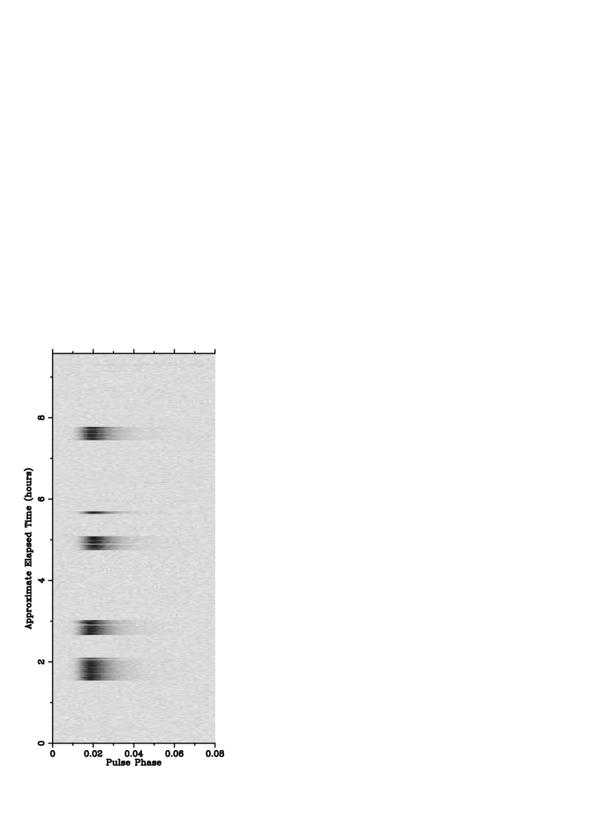
(a) 20 cm / Day 1.

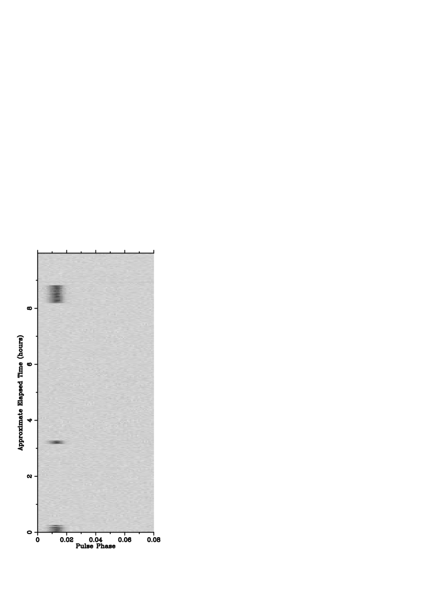
(b) 10 cm / Day 2.

Figure 5: The phase-resolved intensity (arbtirary units) obtained during the two days of long-track observations, demonstrating the stochastic nature of the intermittency.

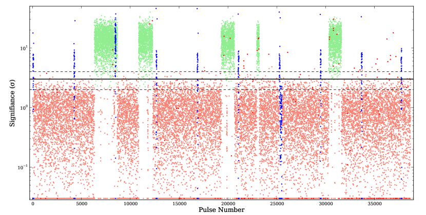
Figure 6: $\sqrt{\mathrm{TS}}$ for 20 cm single pulse profiles. “ON” (green) and “OFF” (salmon) are classified according to the algorithm described in the text. Values with $\sqrt{\mathrm{TS}}<0.1$ are set to 0.1 $\sigma$ for display purposes and appear at the bottom of the figure. Pulses affected by the presence of the calibrator are coloured in blue, while those flagged as suffering from impulsive RFI are drawn in red. The solid black line is drawn at 3$\sigma$, the dashed lines at 2$\sigma$ and 4$\sigma$. In rotations, the five active states measure 2363, 1436, 1352, 263, and 1320, the intervening inactive states 2172, 7019, 2285, and 7105, and the bookending inactive states $>$6320 and $>$7059.

3.5 Time-resolved Active States

3.5.1 Active/Inactive Duty Cycle

During the 20 cm observations of Day 1, the pulsar switched on for five discrete APs with durations given in Figure 6; see also Figure 5. Including only complete active and inactive intervals, the mean AP lasts 1347 rotations, or 1196 s, while the mean IP lasts 4645 rotations, or 4124 s, consistent with our estimates in §2.4, albeit with much poorer statistics. Since the bounding nulls must be at least as long as the observed values, including these intervals increases the mean null duration to $>$4729 s.

On Day 2 (10 cm and 50 cm observations), we observed only two full APs (durations of 450 s and 2220 s; see Figure 5) and one partial AP at the onset of the observation ($>$870 s). The IPs within the observation were much longer (9960 s and 16,980 s) than those of Day 1. The IP/AP duty cycle observed during the long track observations disfavour a memoryless activation process, as there appear to be no short IPs.

3.5.2 AP Nulling

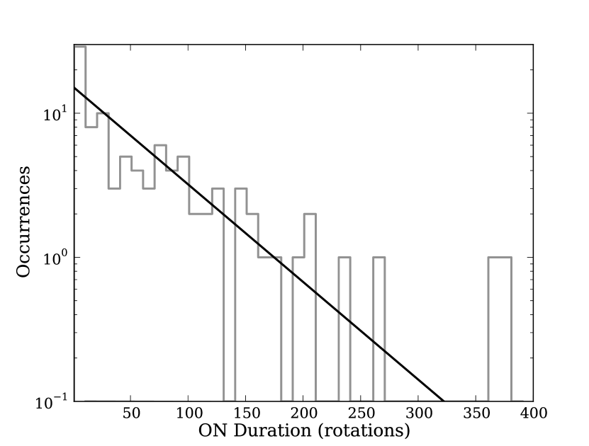
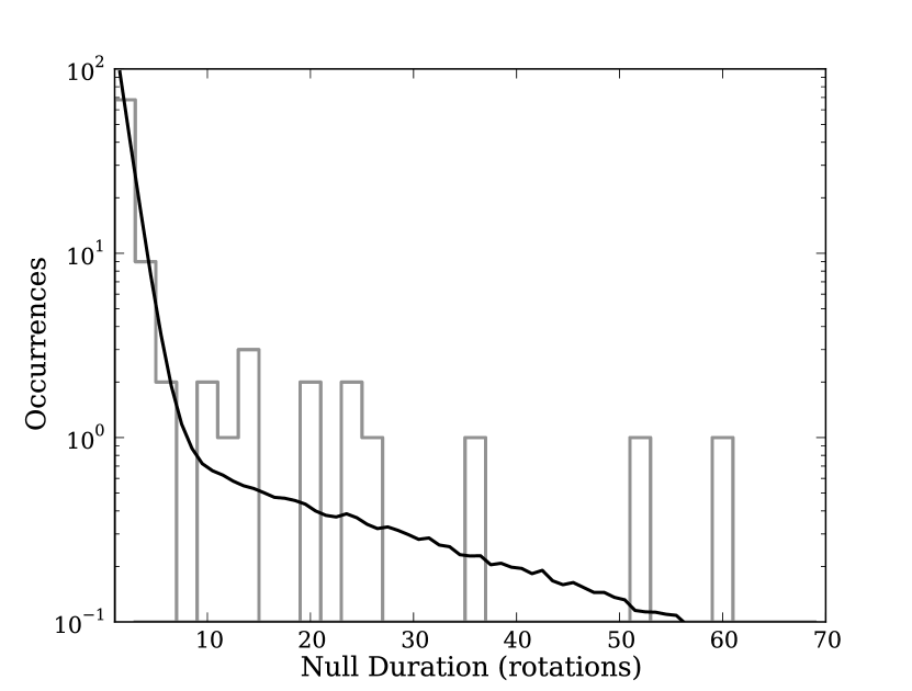
Figure 7: Duration of non-nulling (grey, left) and nulling (grey, right) intervals during active periods. The non-nulling durations are shown with the best-fit exponential distribution overplotted in black, while the model shown in black in the right panel is the mean value from simulations from a two-state Markov model described in §3.5.3.

Within APs, PSR J1717$-$4054 continues to null. To identify null pulses, we derived an analytic template from the high S/N 20 cm profile described above, and we fit this template to each single pulse. Although we noted some variation in pulse shape, the mean profile was generally an acceptable description of the single pulse emission. We estimated the baseline from the offpulse mean, and the phase was known from the timing solution, leaving the signal strength, $s$, of the template in each pulse as the only free parameter. We adopted twice the log likelihood ratio for $s=\hat{s}$, the best-fit value, versus $s=0$ as our test statistic (TS), setting $\mathrm{TS}=0$ when $\hat{s}<=0$. In the absence of a signal, $\mathrm{TS}=0$ half of the time, while the remaining $\mathrm{TS}>0$ values follow a $\chi^{2}$ distribution with one degree of freedom. Then, $\sqrt{\mathrm{TS}}=\sigma$, i.e. the chance probability to observe $\mathrm{TS}\geq\sigma$ is the tail probability of a standard normal distribution integrated from $Z=\sigma$.

By examining data from the long null periods, we found the mean TS to be about 10% higher than expectations, but that rescaling by $0.9$ gave excellent agreement with the expected $\chi^{2}$ distribution. This modified TS, expressed in $\sigma$ units, is calculated for each single pulse and shown in Figure 6. Note that we only expect about 3 pulses in 1000 from the IP to exceed a TS of 3$\sigma$, which is roughly the rate we observe. To identify nulls within the APs, we apply the following classification:

• any pulse with $\mathrm{TS}>4\sigma$ belongs to an AP, as the chance of a null pulse exceeding this threshold is negligible;

• any pulse with TS below $2\sigma$ is a null; although this threshold is arbitrary, since the TS distribution in the alternative hypothesis has an unknown distribution, we justify it below;

• if a pulse has $2\sigma<\mathrm{TS}<3\sigma$, it is a null unless both adjacent pulses are from an AP;

• if a pulse has $3\sigma<\mathrm{TS}<4\sigma$, it belongs to an AP unless both adjacent pulses are nulls.

Using this classification, within the APs, we observed a total of 6281 pulses and 458 nulls, for an active period nulling fraction of $6.8\pm 0.3$%.

3.5.3 AP Null Duration Distribution

The distribution of null and non-null durations within the APs is shown in Figure 7. The distribution of non-null durations is approximately exponential, indicating that the pulsar does not “remember” how long it has been shining since the previous null. The slight excess of short “on” states relative to the model may stem from incorrect classification of a pulse as a null (though see below).

The distribution of nulls, on the other hand, is poorly fit by an exponential, and appears to be bimodal. Short nulls of a few rotations (Type I as classified by Backer, 1970b) significantly outnumber the longer (Type II) nulls extending for tens of rotations. Since the TS distributions of null and non-null pulses are not perfectly separated, some of the Type I nulls may simply be faint pulses. To check this, we co-added the 52 single-pulse nulls and found TS$=3.58\sigma$, indicating that a few of the nulls may be pulses, but that the majority are bona fide nulls. A similar analysis of 16 two-pulse nulls yields TS$=0$, while co-adding Type II nulls with durations of $>5$ rotations yields TS$=3.1$, indicating the long nulls may include a few faint pulses.

To further characterize the nulling process, we attempted to model it as a three-state Markov process following Cordes (2013). In such a process, the probability for the system to switch from one state to another is described by a transition matrix $Q$. The diagonal entries $q_{ii}$ give the probability for the system to remain in its current state and are related to the mean occupancy time of a state; the off-diagonal elements are transition frequencies. In general, such a process produces monotonically decreasing distributions of state occupancy times, tending to exponential distributions as $q_{ii}\rightarrow 1$. Using the observed values for null duration and frequency, we adopted a transition matrix

$$Q=\begin{pmatrix}0.9844&0.0137&0.0019\\ 0.5848&0.4142&0.0000\\ 0.0386&0.0000&0.9614\end{pmatrix},$$

i.e. a single “on state” (state 0) and a short-lived (state 1) and a long-lived (state 2) null state. The observational indistinguishability of states 1 and 2 is represented by a forbidden transition $q_{12}=q_{21}=0$. We simulated many realisations of the process and show the resulting distribution of null durations in Figure 7. The three-state Markov model is largely acceptable, though it fails to reproduce the gap observed between the short-lived and long-lived nulls. (This is a general property of such models, as the probability density function for the duration of any state monotonically decreases.)

3.5.4 Single Pulse Flux Density Distribution

The value of $s$ we obtained to determine TS corresponds directly to the flux density of each single pulse, modulo some scatter from pulse-to-pulse profile variations. The distribution of AP pulse flux densities, excluding pulses affected by RFI and scaled to the measured mean flux (5.2 mJy), appears in Figure 8. The nulls form a narrow normal distribution peaked about zero. This distribution appears identical to the flux density distribution obtained from IPs (not shown), which is exceedingly gaussian and has an r.m.s. of 0.39 mJy. The flux density distribution from non-null pulses, with its high-flux tail, appears to be approximately lognormal, though we note there is a slight underrepresentation of faint pulses relative to that model. Because the variance of the IP distribution is small compared to the non-null distribution (r.m.s. 2.05 mJy), the observed distribution is a good proxy for the intrinsic distribution of single pulse fluxes.

3.5.5 Pulse-to-pulse Correlations

Finally, we searched the data for evidence of correlations between pulses, e.g. as from drifting subpulses. As the relatively modest S/N and the narrow pulse window preclude direct detection of subpulses, we instead searched directly for periodicity in the power spectral density (PSD) of the single pulse fluxes. However, the PSD of each of the APs was consistent with white noise, and we conclude there is no measurable correlation between pulses. Likewise, we looked for any correlation between null duration and the flux of the preceeding/following pulses, e.g. as in that of PSR B1944$+$17 (e.g. Deich et al., 1986). There is no evidence of correlation, save perhaps that the first pulse of an AP tends to be weaker than average.

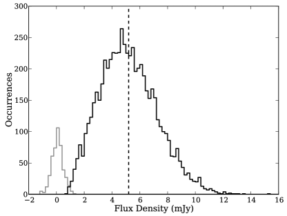
Figure 8: Distribution of observed single pulse flux densities; those identified as nulls are shown in grey, while those identified as non-nulls are drawn in black. The mean flux, 5.2 mJy, is indicated by the dashed vertical line.

4 Summary and Discussion

In summary, we find PSR J1717$-$4054 is well described as a four-state system: an “active” state (0) with nulls at two discrete timescales (1 and 2) and no evidence of complex pulse substructure or memory across nulls; and an “inactive state” (3) whose emission, if present, must be at least 1,000 times fainter than that of state 0. It remains unclear if any of the null states (1, 2, and 3) correspond to the same magnetospheric configuration. The stability of the pulsar’s flux density and profile over timescales of years, as well as the absence of pecularities in its timing solution, suggest the pulsar is stable when averaged over many state transitions, i.e. more than a few days.

The distribution of durations of both APs and IPs has a large scatter, but due to the lack of short APs and (especially) short IPs, each appears to have an intrinsic timescale—that is, neither switching process is memoryless. The complete APs and IPs in our two long-track observations have mean values of 1240 s and 7240 s, respectively, and standard deviations of 690 s and 5160 s, indicating a fairly white spectrum for the IPs and a redder spectrum for the APs. Both timescales are difficult to reconcile with any typical magnetospheric process, and a more likely scenario is a switch between two metastable states triggered by a quasiperiodic perturbation. For example, Cordes & Shannon (2008) have proposed that circumpulsar debris from supernova fallback disks might perturb a pulsar’s magnetosphere, particularly the outer gaps (Cheng, Ho & Ruderman, 1986) or the equatorial disk of return current (e.g. Spitkovsky, 2006). Such a disk could lie well below our limits on reflection (§3.2) but still source asteroids which plunge into the magnetosphere every few hours and provide enough ionized material to substantially alter the current flow. Although the ionized material would only persist for about a rotation, the magnetosphere would at that point have settled into a new metastable state. In this picture, short AP nulls are simply due to plasma fluctuations or patchy emission, an interpretation supported by the approximately exponential distribution of “on” intervals. The longer ($\sim$10 rotation) nulls, however, likely represent a state switch, and may represent an intermediate state between active and inactive states: if the long nulls and IPs correspond to identical magnetospheric configurations, the absence of nulls of of intermediate lengths (few hundred rotations) is puzzling.

Although we cannot directly measure the difference in spindown rate between APs and IPs, we can estimate the contribution of such switching to the r.m.s. of the TOA residuals to our timing solution (Figure 1). Following Equation 12 of Cordes (2013) and using the measured state durations of 1100 s (active) and 4300 s (inactive) and the corresponding state probabilities 0.2 and 0.8, the estimated contribution $\sigma\approx 1.7\,\mathrm{ms}\,\delta\dot{\nu}/\dot{\nu}$. For the observed r.m.s. $\approx 16$ ms, this implies $\delta\dot{\nu}/\dot{\nu}\approx 9$, somewhat larger than values measured from intermittent pulsars (1.5–2.5), implying other sources of timing noise are also important, though Timokhin (2010) suggests that relative spindown rates may depend sensitively on small changes in magnetosphere geometry.

With the measurement of $\dot{\nu}$ we can now place PSR J1717$-$4054 in the context of other nulling pulsars. Despite having one of the highest known NFs, the spindown luminosity ($2\times 10^{32}$ erg s^-1) and characteristic age (3.8 Myr) of PSR J1717$-$4054 are entirely unremarkable. C.f., e.g., Table 1 of Wang, Manchester & Johnston (2007). On the other hand, Biggs (1992), in an analysis of 43 nulling pulsars, found a strong (but scattered) correlation between NF and pulse period, and Wang, Manchester & Johnston (2007) observe a modest correlation with age. Thus, the high NF of PSR J1717$-$4054 is somewhat anomalous. As noted by Cordes & Shannon (2008), large NFs seems to occur at shallow magnetic inclinations, implying PSR J1717$-$4054 may have a magnetic inclination $<$45°. Excluding the very long nulling (intermittent) pulsars such as PSR B1931$+$24, PSR J1717$-$4054 also has one of the longest inactive periods. If, on the other hand, one only considers nulling within active periods, the NF drops to a much more modest 6.8%, in line with many of the other nullers.

It is useful to compare PSR J1717$-$4054 directly with a few other high NF pulsars with long nulls. In particular, recent work by Gajjar, Joshi & Wright (2014) details the properties of PSRs J1738$-$2330 and J1752$+$2359, both with NFs near 90%. Strikingly, both pulsars exhibit features that seem to be absent in our similarly sensitive observations: correlated burst onsets, a decline in flux over time within a burst, and evidence of emission during the long nulls. In contrast, PSR J1717$-$4054 seems simply to switch on and off. Likewise, PSR B1944$+$17 (Kloumann & Rankin, 2010) sports a high (nearly 70%) NF with nulls up to $\sim$100 periods. Its null frequency peaks at one rotation, however, suggesting the short nulls may be due to a carousel pattern. This may be the case for PSR J1717$-$4054, though we have no additional evidence through subpulse structure. Finally, it is also worth pointing out PSR J1502–5653, a scaled Doppelgänger of PSR J1717$-$4054; its $\mathrm{\dot{E}}$ and $\tau_{c}$ agree to within a factor of two, and its NF is similarly high, 93% (Wang, Manchester & Johnston, 2007). It, too, displays a pattern of IP/nulling AP, save with IP and AP durations scaled down by a factor of 10, making it a tempting target for long-track study.

In conclusion, we now have a detailed picture of PSR J1717$-$4054 on all timescales of interest and have also measured a panoply of important properties. Substantial advance—e.g., identifying pulse substructure—must likely await the the large collecting area of the SKA, though some interim progress might be made with, e.g., ultrawide bandwidth feeds, or with additional long-track observations. The identification of nulling at three timescales (few pulses, tens of pulses, and thousands of pulses) is challenging to interpret in any single picture, and we hope these observations will stimulate the introduction of new physical models for state switching.

References

- Baars et al. (1977) Baars J. W. M., Genzel R., Pauliny-Toth I. I. K., Witzel A., 1977, A&A, 61, 99
- Backer (1970a) Backer D. C., 1970a, Nature, 228, 752
- Backer (1970b) Backer D. C., 1970b, Nature, 228, 42
- Biggs (1992) Biggs J. D., 1992, ApJ, 394, 574
- Camilo et al. (2012) Camilo F., Ransom S. M., Chatterjee S., Johnston S., Demorest P., 2012, ApJ, 746, 63
- Cheng, Ho & Ruderman (1986) Cheng K. S., Ho C., Ruderman M., 1986, ApJ, 300, 500
- Cordes (2013) Cordes J. M., 2013, ApJ, 775, 47
- Cordes & Lazio (2002) Cordes J. M., Lazio T. J. W., 2002, ArXiv Astrophysics e-prints
- Cordes & Shannon (2008) Cordes J. M., Shannon R. M., 2008, ApJ, 682, 1152
- Deich et al. (1986) Deich W. T. S., Cordes J. M., Hankins T. H., Rankin J. M., 1986, ApJ, 300, 540
- Deshpande & Rankin (1999) Deshpande A. A., Rankin J. M., 1999, ApJ, 524, 1008
- Gaensler & Slane (2006) Gaensler B. M., Slane P. O., 2006, ARA&A, 44, 17
- Gajjar, Joshi & Wright (2014) Gajjar V., Joshi B. C., Wright G., 2014, MNRAS, 439, 221
- Granet et al. (2005) Granet C. et al., 2005, IEEE Antennas Propagation Magazine, 47, 13
- Herfindal & Rankin (2007) Herfindal J. L., Rankin J. M., 2007, MNRAS, 380, 430
- Hermsen et al. (2013) Hermsen W. et al., 2013, Science, 339, 436
- Hobbs et al. (2004) Hobbs G. et al., 2004, MNRAS, 352, 1439
- Hobbs et al. (2009) Hobbs G. et al., 2009, Publ. Astron. Soc. Australia, 26, 468
- Hobbs et al. (2011) Hobbs G. et al., 2011, Publ. Astron. Soc. Australia, 28, 202
- Hobbs, Edwards & Manchester (2006) Hobbs G. B., Edwards R. T., Manchester R. N., 2006, MNRAS, 369, 655
- Hollow et al. (2008) Hollow R. et al., 2008, in Astronomical Society of the Pacific Conference Series, Vol. 400, Preparing for the 2009 International Year of Astronomy: A Hands-On Symposium, Gibbs M. G., Barnes J., Manning J. G., Partridge B., eds., p. 190
- Hotan, van Straten & Manchester (2004) Hotan A. W., van Straten W., Manchester R. N., 2004, Publ. Astron. Soc. Australia, 21, 302
- Johnston et al. (1992) Johnston S., Lyne A. G., Manchester R. N., Kniffen D. A., D’Amico N., Lim J., Ashworth M., 1992, MNRAS, 255, 401
- Kloumann & Rankin (2010) Kloumann I. M., Rankin J. M., 2010, MNRAS, 408, 40
- Kramer et al. (2006) Kramer M., Lyne A. G., O’Brien J. T., Jordan C. A., Lorimer D. R., 2006, Science, 312, 549
- Lorimer et al. (2012) Lorimer D. R., Lyne A. G., McLaughlin M. A., Kramer M., Pavlov G. G., Chang C., 2012, ApJ, 758, 141
- Lyne et al. (2010) Lyne A., Hobbs G., Kramer M., Stairs I., Stappers B., 2010, Science, 329, 408
- Manchester et al. (2013) Manchester R. N. et al., 2013, Publ. Astron. Soc. Australia, 30, 17
- Phillips, Thorsett & Kulkarni (1993) Phillips J. A., Thorsett S. E., Kulkarni S. R., eds., 1993, Astronomical Society of the Pacific Conference Series, Vol. 36, Planets around pulsars; Proceedings of the Conference, California Inst. of Technology, Pasadena, Apr. 30-May 1, 1992
- Rankin & Wright (2008) Rankin J. M., Wright G. A. E., 2008, MNRAS, 385, 1923
- Spitkovsky (2006) Spitkovsky A., 2006, ApJ, 648, L51
- Staveley-Smith et al. (1996) Staveley-Smith L. et al., 1996, Publ. Astron. Soc. Australia, 13, 243
- Timokhin (2010) Timokhin A. N., 2010, MNRAS, 408, L41
- Unwin et al. (1978) Unwin S. C., Readhead A. C. S., Wilkinson P. N., Ewing W. S., 1978, MNRAS, 182, 711
- van Straten & Bailes (2011) van Straten W., Bailes M., 2011, Publ. Astron. Soc. Australia, 28, 1
- Wang, Manchester & Johnston (2007) Wang N., Manchester R. N., Johnston S., 2007, MNRAS, 377, 1383
- Wilson et al. (2011) Wilson W. E. et al., 2011, MNRAS, 416, 832
Acknowledgments
We thank the anonymous referee and the journal editors, whose effort and input improved this paper.
The Parkes radio telescope and Australia Telescope Compact Array are part of the Australia Telescope, which is funded by the Commonwealth Government for operation as a National Facility managed by CSIRO.
PULSE@Parkes is funded by CSIRO Astronomy and Space Science. We are grateful to the Australia-Japan Foundation, the Victorian Space Science Education Centre, SPICE at the University of Western Australia, the Astrophysics groups at the University of Cardiff and University of Oxford, ASTRON, NAOJ Mizusawa VLBI Observatory, Koriyama Space Park, Penrith Anglican College, and the University of Brownsville, Texas for support in funding and hosting sessions. The authors would like to acknowledge the more than 1,100 students from 93 schools who have taken part in sessions and contributed to the data gathering since the program’s inception in December 2007, as well as the CSIRO Astronomy and Space Science staff, visitors, and co-supervised PhD students whose volunteer participation has enriched the program.