Zeros of Networked Systems with Time-invariant Interconnections

Abstract

This paper studies zeros of networked linear systems with time-invariant interconnection topology. While the characterization of zeros is given for both heterogeneous and homogeneous networks, homogeneous networks are explored in greater detail. In the current paper, for homogeneous networks with time-invariant interconnection dynamics, it is illustrated how the zeros of each individual agent’s system description and zeros definable from the interconnection dynamics contribute to generating zeros of the whole network. We also demonstrate how zeros of networked systems and those of their associated blocked versions are related.

1 Introduction

Recent developments of enabling technologies such as communication systems, cheap computation equipment and sensor platforms have given great impetus to the creation of networked systems. Thus, this area has attracted significant attention worldwide and researchers have studied networked systems from different perspectives (see e.g. [26], [22], [28]). In particular, in view of the recent chain of events [14], [10] and [24], the issues of security and cyber threats to the networked systems have gained growing attention. This paper uses system theoretic approaches to deal with problems involved with the security of networks.

Recent works have shown that control theory can be used as an effective tool to detect and mitigate the effects of cyber attacks on the networked systems; see for example [20], [6], [16], [1], [27], [29] and the references listed therein. The authors of [29] have introduced the concept of zero-dynamics attacks and shown how attackers can use knowledge of networks’ zeros to produce control commands such that they are not detected as security threats. Thus, zeros of networks provide valuable information relevant to detecting cyber attacks. Though various aspects of the dynamics of networked systems have been extensively studied in the literature [23, 21, 11], to the authors’ best knowledge the zeros of networked systems have not been studied in any detail [35].

This paper examines the zeros of networked systems in more depth. Our focus is on networks of finite-dimensional linear dynamical systems that arise through static interconnections of a finite number of such systems. Such models arise naturally in applications of linear networked systems, e.g. for cyclic pursuit [19]; shortening flows in image processing [5], or for the discretization of partial differential equations [4].

Our ultimate goal is to analyze the zeros of networked systems with periodic, or more generally time-varying interconnection topology. An important tool for this analysis is blocking or lifting technique for networks with time-invariant interconnections. Note that blocking of linear time-invariant systems is useful in design of controllers for linear periodic systems as shown by [7] and [18]. References [3], [15], [34] and [8] have analyzed zeros of blocked systems obtained from blocking of time-invariant systems. Their works were extended by [34], [8]. However, these earlier contributions do not take any underlying network structure into consideration. In this paper, we introduce some results that provide a first step in that direction.

The structure of this paper is as follows. First, in Section 2 we introduce state-space and higher order polynomial system models for time-invariant networks of linear systems. A central result used is the strict system equivalence between these different system representations. Moreover, we completely characterize both finite and infinite zeros of arbitrary heterogeneous networks. For homogeneous networks of identical SISO systems more explicit results are provided in Section 3. Homogeneous networks with a circulant coupling topology are studied as well. In Section 4, a relation between the transfer function of the blocked system and the transfer function of the associated unblocked system is explained. We then relate the zeros of blocked networked systems to those of the corresponding unblocked systems, generalizing work by [34], [8],[33]. Finally, Section 5 provides the concluding remarks.

2 Problem Statement and Preliminaries

We consider networks of $N$ linear systems, coupled through constant interconnection parameters. Each agent is assumed to have the state-space representation as a linear discrete-time system

$$\begin{split}x_{i}(t+1)&=A_{i}x_{i}(t)+B_{i}v_{i}(t)\\ w_{i}(t)&=C_{i}x_{i}(t),\;i=1,\dots,N.\end{split}$$ (1)

Here, $A_{i}\in\mathbb{R}^{n_{i}\times n_{i}}$, $B_{i}\in\mathbb{R}^{n_{i}\times m_{i}}$ and $C_{i}\in\mathbb{R}^{p_{i}\times n_{i}}$ are the associated system matrices. We assume that each system is reachable and observable and that the agents are interconnected by static coupling laws

$$v_{i}(t)=\sum_{j=1}^{N}L_{ij}w_{j}(t)+R_{i}u(t)\in\mathbb{R}^{m_{i}}$$

with $L_{ij}\in\mathbb{R}^{m_{i}\times p_{j}}$, $R_{i}\in\mathbb{R}^{m_{i}\times m}$ and $u(t)\in\mathbb{R}^{m}$ denoting an external input applied to the whole network. Further, we assume that there is a $p$-dimensional interconnected output given by

$$y(t)=\sum_{i=1}^{N}S_{i}w_{i}(t)+Du(t)\;\mbox{ with }\;S_{i}\in\mathbb{R}^{p\times p_{i}},\;i=1,\dots,N.$$

Define $\overline{m}=\sum_{i=1}^{N}m_{i}$, $\overline{p}=\sum_{i=1}^{N}p_{i}$, $\overline{n}=\sum_{i=1}^{N}n_{i}$ and coupling matrices

$$L = (L_{ij})_{ij}\in\mathbb{R}^{\overline{m}\times\overline{p}}\quad R=\begin{pmatrix}R_{1}\\ \vdots\\ R_{N}\end{pmatrix}\in\mathbb{R}^{\overline{n}\times m}$$

$$S = (S_{1},\dots,S_{N})\in\mathbb{R}^{p\times\overline{p}}\quad D\in\mathbb{R}^{p\times m}$$

as well as node matrices

$$\begin{split}A&=\mbox{\rm diag}\,(A_{1},\ldots,A_{N}),\quad B=\mbox{\rm diag}\,(B_{1},\ldots,B_{N})\\ C&=\mbox{\rm diag}\,(C_{1},\ldots,C_{N}),\quad x(t):=\begin{pmatrix}x_{1}(t)\\ \vdots\\ x_{N}(t)\end{pmatrix}\in\mathbb{R}^{\overline{n}}.\end{split}$$ (2)

Then the closed-loop system is

$$\begin{split}x(t+1)&={\mathbf{A}}x(t)+{\mathbf{B}}u(t)\\ y(t)&={\mathbf{C}}x(t)+Du(t),\end{split}$$ (3)

with matrices

$$\mathbf{A}:=A+BLC\quad\mathbf{B}:=BR,\quad{\mathbf{C}}:=SC.$$ (4)

One can also start by assuming that each system (1) is defined in terms of Rosenbrock-type equations [25] i.e. by systems of higher order difference equations

$$\begin{array}[]{rcl}T_{i}(\sigma)\xi_{i}(t)&=&U_{i}(\sigma)v_{i}(t)\\ w_{i}(t)&=&V_{i}(\sigma)\xi_{i}(t).\end{array}$$ (5)

Here $\sigma$ denotes the forward shift operator that acts on sequences of vectors $(\xi(t))_{t}$ as $(\sigma\xi(t))=\xi(t+1)$. Furthermore, $T_{i},U_{i},V_{i}$ denote polynomial matrices of sizes $T_{i}(z)\in\mathbb{R}[z]^{r_{i}\times r_{i}},U_{i}(z)\in\mathbb{R}[z]^{r_{i}\times m_{i}}$ and $V_{i}(z)\in\mathbb{R}[z]^{p_{i}\times r_{i}}$, respectively. We always assume that $T_{i}(z)$ is nonsingular, i.e. that $\det T_{i}(z)$ is not the zero polynomial. Moreover, the system (5) is assumed to be strictly proper, i.e. we assume that the associated transfer function

$$\begin{split}G_{i}(z)&=V_{i}(z)T_{i}(z)^{-1}U_{i}(z)\end{split}$$ (6)

is strictly proper. Following Fuhrmann [12], any strictly proper system of higher order difference equations has an associated state-space realization $(A,B,C)$, the so-called shift realization, such that the polynomial matrices

$$\begin{pmatrix}zI-A&-B\\ C&0\\ \end{pmatrix},\quad\begin{pmatrix}T(z)&-U(z)\\ V(z)&0\\ \end{pmatrix}$$ (7)

are strict system equivalent [12]. If the first order representation (1) is strict system equivalent to the higher order system (5) then of course the associated transfer functions coincide, i.e. we have

$$\begin{split}C_{i}(zI-A_{i})^{-1}B_{i}&=V_{i}(z)T_{i}(z)^{-1}U_{i}(z).\end{split}$$ (8)

Throughout this paper we assume that the first order and higher order representations i.e. the systems (1) and (5), are chosen to be of minimal order, respectively. This is equivalent to the controllability and observability of the shift realizations (1) associated with these representations (5). It is also equivalent to the simultaneous left coprimeness of $T_{i}(z),U_{i}(z)$ and the right coprimeness of $T_{i}(z),V_{i}(z)$. Proceeding as above, define polynomial matrices

$$\begin{array}[]{rcl}T(z)&=&\mbox{\rm diag}\,(T_{1}(z),\ldots,T_{N}(z))\in\mathbb{R}[z]^{\overline{r}\times\overline{r}}\\ \end{array}$$ (9)

and similarly for $V(z)$ and $U(z)$. Here $\overline{r}=\sum_{i=1}^{N}r_{i}$. Using this notation, we write all $N$ systems of (5) in the matrix form as

$$\left(\begin{array}[]{c}0\\ I\\ \end{array}\right)w(t)=\left(\begin{array}[]{cc}T(\sigma)&-U(\sigma)\\ V(\sigma)&0\\ \end{array}\right)\left(\begin{array}[]{c}\xi(t)\\ v(t)\\ \end{array}\right),$$ (10)

where $w(t)=\left(\begin{array}[]{cccc}w_{1}(t)^{\top}&w_{2}(t)^{\top}&\ldots&w_{N}(t)^{\top}\\ \end{array}\right)^{\top}$ and similarly for $\xi(t)$ and $v(t)$. Then we have the left- and right coprime factorizations of the $\overline{p}\times\overline{m}$ node transfer function as

$$G(z)=C(zI-A)^{-1}B=V(z)T(z)^{-1}U(z).$$

The interconnections are given, as before, by

$$\begin{array}[]{rcl}v(t)&=&Lw(t)+Ru(t)\\ y(t)&=&Sw(t)+Du(t).\\ \end{array}$$

The resulting network representation then becomes

$$\left(\begin{array}[]{c}0\\ I\\ \end{array}\right)y(t)=\left(\begin{array}[]{cc}T(\sigma)-U(\sigma)LV(\sigma)&-U(\sigma)R\\ SV(\sigma)&D\\ \end{array}\right)\left(\begin{array}[]{c}\xi(t)\\ u(t)\\ \end{array}\right)$$ (11)

with the $p\times m$ network transfer function defined as

$$\begin{split}\Gamma(z)&=\mathbf{C}(zI-\mathbf{A})^{-1}\mathbf{B}+D\\ &=SV(z)(T(z)-U(z)LV(z))^{-1}U(z)R+D.\end{split}$$ (12)

The connection between the state-space and the polynomial matrix representations (3) and (11), respectively, is clarified by the following result. This theorem implies that important system-theoretic properties such as reachability and observability, as well as the poles and zeros of the networked system (3) can all be characterized by the polynomial system matrix (11).

Theorem 1 ([13]).

The interconnected systems (3) and (11) are strict system equivalent. In particular, for each $q\geq\max(\overline{n},\overline{r})$ there exist unimodular polynomial matrices $E(z),F(z)$ such that

$$\begin{split}&E(z)\begin{pmatrix}I_{q-\overline{n}}&0&0\\ 0&zI-\mathbf{A}&-\mathbf{B}\\ 0&\mathbf{C}&D\\ \end{pmatrix}F(z)=\\ &\begin{pmatrix}I_{q-\overline{r}}&0&0\\ 0&T(z)-U(z)LV(z)&-U(z)R\\ 0&SV(z)&D\\ \end{pmatrix}.\end{split}$$

As a consequence of Theorem 1 we derive a complete characterization for the zeros of the system (3). We first present an extension of the classical definition of the zeros [17] to the higher order system (5). Note that the normal rank $\mbox{\rm grk}\,\>G(z)$ of a rational matrix function $G(z)$ is defined as

$$\mbox{\rm grk}\,\;G(z)=\max\{\mbox{\rm rank}\,\;G(z)\;|\;z\in\mathbb{C},G(z)\neq\infty\}.$$

Definition 1.

Let $U(z),V(z),T(z)$ be polynomial matrices with $T(z)\in\mathbb{R}[z]^{\overline{r}\times\overline{r}}$ nonsingular such that the $\overline{p}\times\overline{m}$ node transfer function $V(z)T(z)^{-1}U(z)$ is strictly proper; let $D$ be a constant matrix. A finite zero of the polynomial system matrix

$$\Pi(z)=\begin{pmatrix}T(z)&-U(z)\\ V(z)&D\\ \end{pmatrix}$$ (13)

is any complex number $z_{0}\in\mathbb{C}$ such that

$$\mbox{\rm rank}\,\;\Pi(z_{0})<\mbox{\rm grk}\,\;\Pi(z)$$

holds. $\Pi(z)$ is said to have a zero at infinity if

$$\overline{r}+\mbox{\rm rank}\,\;D<\mbox{\rm grk}\,\;\Pi(z).$$

As a consequence of Fuhrmann’s result [12], a polynomial system matrix (13) has a finite or infinite zero if and only if the polynomial matrix

$$\Sigma(z)=\begin{pmatrix}zI-A&-B\\ C&D\\ \end{pmatrix}$$

of the associated shift realization $(A,B,C,D)$ has a finite or infinite zero. Theorem 1 thus leads to a complete characterization of the zeros for the interconnected system (3) as stated in the subsequent theorem. We emphasize that the characterization of the zeros in the subsequent Theorem 2 holds for any interconnection matrices and does not require any assumptions on reachability or observability of the network, except of those for the individual node systems.

Theorem 2 ([13]).

Consider the strictly proper node transfer function $G(z)$ with minimal representations (2) as

$$G(z)=C(zI-A)^{-1}B=V(z)T(z)^{-1}U(z).$$

Let $L,R,S,D$ be any arbitrary constant interconnection matrices of the proper dimensions and

$$\Gamma(z)=SV(z)(T(z)-U(z)LV(z))^{-1}U(z)R+D$$

denote the network transfer function. Assume that $G(z)$ is represented by a polynomial left coprime matrix fraction description (MFD) as

$$G(z)=D^{-1}_{L}(z)N_{L}(z).$$

Then

1. For all $z\in\mathbb{C}$

   $$\begin{split}&\mbox{\rm rank}\,\left(\begin{array}[]{cc}zI-\mathbf{A}&-\mathbf{B}\\ \mathbf{C}&D\end{array}\right)\\ &=\overline{n}-\overline{r}+\mbox{\rm rank}\,\left(\begin{array}[]{cc}T(z)-U(z)LV(z)&-U(z)R\\ SV(z)&D\\ \end{array}\right).\end{split}$$

2. For all $z\in\mathbb{C}$

   $$\begin{split}&\mbox{\rm rank}\,\left(\begin{array}[]{cc}zI-A-BLC&-BR\\ SC&D\end{array}\right)\\ &=\overline{n}-\overline{p}+\mbox{\rm rank}\,\left(\begin{array}[]{cc}D_{L}(z)-N_{L}(z)L&-N_{L}(z)R\\ S&D\\ \end{array}\right).\end{split}$$

3. $(\mathbf{A},\mathbf{B},\mathbf{C},D)$ has a finite zero at $z_{0}\in\mathbb{C}$ if and only if

   $$\begin{split}&\mbox{\rm rank}\,\left(\begin{array}[]{cc}T(z_{0})-U(z_{0})LV(z_{0})&-U(z_{0})R\\ SV(z_{0})&D\\ \end{array}\right)<\\ &\overline{r}+\mbox{\rm grk}\,\;\Gamma(z).\end{split}$$

4. $(A+BLC,BR,SC,D)$ has a zero at infinity if and only if

   $$\mbox{\rm rank}\,\;D<\mbox{\rm grk}\,\;\Gamma(z).$$

   In particular, if $D$ has full-row rank or full-column rank, then $(A+BLC,BR,SC,D)$ has no infinite zero.

3 Zeros of Homogeneous Networks

The preceding result has a nice simplification in the case of homogeneous networks of SISO agents, i.e. where the node systems $(A_{i},B_{i},C_{i})$ are single input single output systems with identical transfer function. Let us define the interconnection transfer function as

$$\phi(z)=S(zI-L)^{-1}R+D.$$

The next theorem relates the zeros of the system (3) to those of the interconnection dynamics defined by the quadruple $(L,R,S,D)$. Before we provide this main result, we need to state the following lemma regarding the generic rank of $\Gamma(z)$.

Lemma 1.

Assume that $(A_{i},b_{i},c_{i})$ are scalar SISO systems with identical transfer function $g(z)=c_{i}(zI-A_{i})^{-1}b_{i}$. Let $L,R,S,D$ denote any constant interconnection matrices of the proper dimensions and $\phi(z)=S(zI-L)^{-1}R+D$ be the interconnection transfer function. Then the following equality holds.

$$\mbox{\rm grk}\,\;\Gamma(z)=\mbox{\rm grk}\,\;\phi(z).$$

Proof. Consider any coprime factorization $g(z)=\frac{p(z)}{q(z)}$ of the strictly proper transfer function $g(z)$, having McMillan degree $n$. Define $h(z)=g(z)^{-1}=\frac{q(z)}{p(z)}$. We know that

$$\begin{split}\mbox{\rm grk}\,\;\Gamma(z)&=\mbox{\rm grk}\,\left(\begin{array}[]{cc}zI-\mathbf{A}&-\mathbf{B}\\ \mathbf{C}&D\end{array}\right)-nN\\ \end{split}$$ (14)

Then by applying the second part of Theorem 2, one obtains

$$\begin{split}&\mbox{\rm grk}\,\left(\begin{array}[]{cc}zI-\mathbf{A}&-\mathbf{B}\\ \mathbf{C}&D\end{array}\right)=\\ &N(n-1)+\mbox{\rm grk}\,\left(\begin{array}[]{cc}q(z)I_{N}-p(z)L&-p(z)R\\ S&D\\ \end{array}\right)=\\ &N(n-1)+\mbox{\rm grk}\,\left(\begin{array}[]{cc}h(z)I_{N}-L&-R\\ S&D\\ \end{array}\right)=\\ &N(n-1)+\mbox{\rm grk}\,\left(\begin{array}[]{cc}\eta I_{N}-L&-R\\ S&D\\ \end{array}\right)=\\ &Nn+\mbox{\rm grk}\,\;\phi(z).\end{split}$$ (15)

By substituting the last equality of (15) into (14), the result follows.

$\square\$

Theorem 3.

Assume that $(A_{i},b_{i},c_{i})$ are SISO systems with identical transfer function $g(z)=c_{i}(zI-A_{i})^{-1}b_{i}$.Then $(\mathbf{A},\mathbf{B},\mathbf{C},D)$ has a zero at infinity if and only if $(L,R,S,D)$ has a zero at infinity.

Proof. By Lemma 1, the network transfer function matrix $\Gamma(z)$ and the interconnection transfer matrix $\phi(z)$ have the same normal rank. Using the conclusion of Theorem 2 (part 4), the result follows. $\square\$

Theorem 3 shows that the infinite zero structure of a homogeneous network depends only upon the interconnection parameters and not on the specific details of the node transfer function. This is in contrast to the finite zero structure, as is shown by the following result.

Theorem 4.

Assume that $(A_{i},b_{i},c_{i})$ are SISO systems with identical transfer function $g(z)=c_{i}(zI-A_{i})^{-1}b_{i}$. Let $p(z)/q(z)$ be a coprime polynomial factorization of $g(z)$ and define $h(z)=g(z)^{-1}$. Let $(L,R,S,D)$ denote any constant interconnection matrices of the proper dimensions.

1. $(\mathbf{A},\mathbf{B},\mathbf{C},D)$ has a finite zero at $z_{0}\in\mathbb{C}$ with $p(z_{0})\neq 0$ if and only if $h(z_{0})\in\mathbb{C}$ is a finite zero of $(L,R,S,D)$.

2. $(\mathbf{A},\mathbf{B},\mathbf{C},D)$ has a finite zero at $z_{0}\in\mathbb{C}$ with $p(z_{0})=0$ if and only if $(L,R,S,D)$ has a zero at infinity.

Proof. We first prove the first part of the theorem. By Lemma 1 and Theorem 2, $z_{0}\in\mathbb{C}$ is a zero of $(\mathbf{A},\mathbf{B},\mathbf{C},D)$ if and only if

$$\mbox{\rm rank}\,\left(\begin{array}[]{cc}q(z_{0})I_{N}-p(z_{0})L&-p(z_{0})R\\ S&D\\ \end{array}\right)<N+\mbox{\rm grk}\,\;\phi(z).$$ (16)

For $p(z_{0})\neq 0$ this is equivalent to

$$\mbox{\rm rank}\,\left(\begin{array}[]{cc}h(z_{0})I_{N}-L&-R\\ S&D\\ \end{array}\right)<N+\mbox{\rm grk}\,\;\phi(z),$$

i.e. $h(z_{0})$ being a finite zero of $(L,R,S,D)$. For the second part note that $z_{0}\in\mathbb{C}$ is a zero of $(\mathbf{A},\mathbf{B},\mathbf{C},D)$ if and only if inequality (16) holds. If $p(z_{0})=0$, then by coprimeness of $p(z)$ and $q(z)$ we have $q(z_{0})\neq 0$ and therefore (16) is equivalent to

$$N+\mbox{\rm rank}\,D=\mbox{\rm rank}\,\left(\begin{array}[]{cc}q(z_{0})I_{N}&0\\ S&D\\ \end{array}\right)<N+\mbox{\rm grk}\,\;\phi(z).$$

This is equivalent to $\mbox{\rm rank}\,\;D<\mbox{\rm grk}\,\;\phi(z)$. Thus a zero of the node transfer function $g(z)$ is a zero of $(\mathbf{A},\mathbf{B},\mathbf{C},D)$ if and only if $(L,R,S,D)$ has a zero at infinity. This completes the proof. $\square\$

Now assume that $D$ has full-column rank or full-row rank. Then the homogeneous network realization $(\mathbf{A},\mathbf{B},\mathbf{C},D)$ has no zeros at infinity. Thus in this case the finite zeros of $(\mathbf{A},\mathbf{B},\mathbf{C},D)$ are exactly the preimages of the finite zeros of $(L,R,S,D)$ under the rational function $h(z)$. We conclude with a result that is useful for the design of networks with prescribed zero properties. The result below bears a certain similarity with a result by Fax and Murray [11]. As shown by them, a formation of $N$ identical vehicles can be analyzed for stability by analyzing a single vehicle with the same dynamics modified by only a scalar, which assumes values equal to the eigenvalues of the interconnection matrix. Such a result is to do with poles, linking those of the individual agent and the overall system via the eigenvalues (which are pole-like) of the interconnection matrix. Our result is to do with the zeros, but still links those of the individual agent, those of the interconnection matrix (suitably interpreted) and those of the whole system.

With the help of the preceding results, we can now study two other important properties of networks, namely, losslessness and passivity. It is well known, see e.g. [31] (Section II. B), that if all agent transfer function matrices and the system defined by the quadruple $(L,R,S,D)$ are lossless, then the system (3) is lossless. We now provide an improvement of this result for the case of SISO agents.

Recall that a strictly proper real rational transfer function $g(z)$ is called lossless [30] if all poles of $g(z)$ are in the open unit disc and $|g(z)|=1$ holds for all $|z|=1$. A key property used below is that $|g(z)|>1$ if $|z|<1$ and $|g(z)|<1$ if $|z|>1$.

Theorem 5.

Assume that $D$ has full-column rank or full-row rank. Then

1. The homogeneous network $(\mathbf{A},\mathbf{B},\mathbf{C},D)$ has no zeros at infinity. A complex number $z_{0}$ is a finite zero of $(\mathbf{A},\mathbf{B},\mathbf{C},D)$ if and only if $h(z_{0})\neq\infty$ is a finite zero of $(L,R,S,D)$.

2. Assume that the agent transfer function $g(z)$ is lossless. Then $(\mathbf{A},\mathbf{B},\mathbf{C},D)$ is a minimum phase network, i.e. all of its zeros have absolute value $<1$, if and only if $(L,R,S,D)$ is minimum phase.

Proof. The first claim is an immediate consequence of Theorem 4. If $g(z)$ is lossless then $|g(z)|<1$ holds if and and only if $|z|>1$. Thus $h(z)=1/g(z)$ maps the complement of the open unit disc onto itself. Thus $|z|\geq 1$ if and only if $|h(z)|\geq 1$. Therefore $(L,R,S,D)$ has a finite zero $\eta_{0}$ with $|\eta_{0}|\geq 1$ if and only if each $z$ with $h(z)=\eta_{0}$ satisfies $|z|\geq 1$ and is a zero of $(\mathbf{A},\mathbf{B},\mathbf{C},D)$. Note that for any finite $\eta_{0}$, there is necessarily a $z$ satisfying $h(z)=\eta_{0}$, since this is a polynomial equation for $z$. This proves the result. $\square\$

We now extend the second part of the above corollary for the choice of passive transfer functions [30]. Let us recall that $g(z)$ is passive if and only if

1. all poles of $g(z)$ are in $|z|\leq 1$

2. $|g(z)|\leq 1$ $\;\forall\;$ $|z|=1$.

This implies

1. $|g(z)|<1$ $\;\forall\;|z|>1$

2. If $|g(z)|>1$, then $|z|<1$.

Corollary 1.

Assume that $D$ has full-column rank or full-row rank and $g(z)$ is passive. Then $(\mathbf{A},\mathbf{B},\mathbf{C},D)$ is a minimum phase network, i.e. all of its zeros have absolute value $<1$, if $(L,R,S,D)$ is minimum phase.

Proof. Suppose $|z_{0}|$ is a finite zero of $\{A,B,C,D\}$. Then $h(z_{0})$ is a finite zero of $(L,S,R,D)$, i.e., $1/g(z_{0})$ is a finite zero of $(L,S,R,D)$. By the minimum phase assumption, $|1/g(z_{0})|<1$ or $|g(z_{0})|>1$. Passivity of $g(z_{0})$ thus implies $|z_{0}|<1$. $\square\$

3.1 Design of Networks

An important issue is the construction of network topologies so that the resulting network is zero-free, i.e. it does not have any finite zeros (but still may have a zero at infinity). We derive a simple sufficient condition for homogeneous networks. By Corollary 5, the homogeneous network $(\mathbf{A},\mathbf{B},\mathbf{C},D)$ is zero-free if and only if $(L,R,S,D)$ is zero-free. For simplicity, we assume that there is a single external input and a single external output associated with the network, i.e. $m=p=1$. Moreover, we assume $D=0$. Thus the interconnection transfer function $\phi(z)=S(zI_{N}-L)^{-1}R$ is scalar strictly proper rational. The next result characterizes which outputs of the SISO interconnected system lead to a network without finite zeros, for given state and input interconnection matrices.

Theorem 6 (SISO Design Condition).

Assume that $(A_{i},b_{i},c_{i})$ are identical minimal SISO systems with identical transfer function. Let $(L,R)$ be reachable with $L\in\mathbb{R}^{N\times N},R\in\mathbb{R}^{N}$. Then a network output $S\in\mathbb{R}^{1\times N}$ defines a minimal network realization $(\mathbf{A},\mathbf{B},\mathbf{C},0)$ without finite zeros if and only if $S(zI_{N}-L)^{-1}R$ has relative degree $N$.

Proof. By Corollary 5, the homogeneous network $(\mathbf{A},\mathbf{B},\mathbf{C},0)$ has no finite zeros if and only if this holds for $(L,R,S,0)$. In the SISO case this is equivalent to the transfer function $S(zI_{N}-L)^{-1}R$ having no zeros. By [13], $(\mathbf{A},\mathbf{B},\mathbf{C},0)$ is minimal if and only if $(L,R,S)$ is minimal. In either case, $S(zI_{N}-L)^{-1}R$ has McMillan degree $N$ and has no zeros if and only if the relative degree of $S(zI_{N}-L)^{-1}R$ is equal to $N$. $\square\$

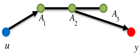
Figure 1: A homogenous network consisting of three SISO agents. The agents, the external input and measurement are depicted by green, blue and red circles, accordingly. The whole network has two zeros at -1 and 1 when all weights are set to unity.

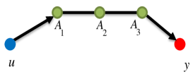
Figure 2: A homogenous network consisting of three SISO agents. The agents, the external input and measurement are depicted by green, blue and red circles, accordingly. The whole network is zero-free when all weights are set to unity.

The above theorem characterizes when the SISO networked systems are zero-free. We note that the condition is equivalent to the sytem-theoretic condition that the closed loop system $(\mathbf{A},\mathbf{B},\mathbf{C},0)$ is feedback irreducible; i.e. that $(\mathbf{A}+\mathbf{B}K,\mathbf{C})$ is observable for all state feedback matrices $K$.

The next example illustrates that the zeros of the system (3) may drastically change by replacing and adding a link.

Example 1.

Consider the network depicted in Fig. 1 where the nodes are simply double integrators. Note that there exist bidirectional links between the agents. By assuming a unit weight on each link, it is easy to verify that for such a network the interconnection matrices are $L=\left(\begin{array}[]{ccc}1&1&0\\ 1&0&1\\ 0&1&1\end{array}\right),R=\left(\begin{array}[]{c}1\\ 0\\ 0\end{array}\right)$ and $S=\left(\begin{array}[]{ccc}0&1&0\end{array}\right)$. Moreover, the interconnection dynamics has a single zero at $z=1$. Hence, by using Theorem 4 it is easy to see that the whole network has two zeros at $1$ and $-1$. One can also observe that by adding an extra link in Fig. 1 from agent $A_{3}$ to the measurement node, with the same set of interconnection matrices as before except for $S$ which assumes random values in its nonzero entries, the whole network becomes zero-free. The same result holds i.e. the resultant network is zero-free, when the topology is modified according to Fig. 2.

3.2 Circulant Homogeneous Networks

Homogeneous networks with special coupling structures appear in many applications, such as cyclic pursuit [19]; shortening flows in image processing [5] or the discretization of partial differential equations [4]. Here, we characterize the zeros for interconnections that have a circulant structure. A homogeneous network is called circulant if the state-to-state coupling matrix $L$ is a circulant, i.e.

$$\begin{split}L&=\rm{Circ}(c_{0},...,c_{N-1})\\ &=\begin{pmatrix}c_{0}&c_{1}&\cdots&c_{N-2}&c_{N-1}\\ c_{N-1}&c_{0}&c_{1}&\cdots&c_{N-2}\\ \vdots&\ddots&\ddots&\ddots&\vdots\\ c_{2}&\cdots&c_{N-1}&c_{0}&c_{1}\\ c_{1}&c_{2}&\cdots&c_{N-1}&c_{0}\end{pmatrix}.\end{split}$$

The book [9] provides algebraic background on the circulant matrices. A basic fact on circulant matrices is that they are simultaneously diagonalizable by the Fourier matrix

$$\Phi=\frac{1}{\sqrt{N}}\begin{pmatrix}1&1&1&\ldots&1\\ 1&\omega&\omega^{2}&\ldots&\omega^{N-1}\\ 1&\omega^{2}&\omega^{4}&\ldots&\omega^{2N-2}\\ \vdots&&&&\\ 1&\omega^{N-1}&\omega^{2N-2}&\ldots&\omega^{(N-1)^{2}}\end{pmatrix}\text{ ,}$$

where $\omega=e^{2\pi j/N}$ denotes a primitive $N-$th root of unity. Note, that $\Phi$ is both a unitary and a symmetric matrix. It is then easily seen that any circulant matrix $L$ has the form $L=\Phi\mbox{\rm diag}\,(p_{L}(1),p_{L}(\omega),\ldots,p_{L}(\omega^{N-1}))\Phi^{*},$ where $p_{L}(z):=\sum_{k=0}^{N-1}c_{k}z^{k-1}.$ As a consequence of the preceding analysis we obtain the following result.

Theorem 7.

Suppose that the system in (3) is a circulant homogeneous network. Let $D$ be full rank and $M=\mbox{\rm diag}\,(p_{L}(1),\ldots,p_{L}(\omega^{N-1}))$ and $w_{1},\ldots,w_{N}$ denote the complex roots of

$$\rm{det}\left(\begin{array}[]{cc}wI_{N}-M&-\Phi^{*}R\\ S\Phi&D\\ \end{array}\right)=0.$$

Then

$$\bigcup_{k=1}^{N}\{z\in\mathbb{C}\;|\;q(z)-w_{k}p(z)=0\}$$

are the finite zeros of the homogeneous network $(\mathbf{A},\mathbf{B},\mathbf{C},D)$.

Proof. By Theorem 4, we conclude that the system defined by $(\mathbf{A},\mathbf{B},\mathbf{C},D)$ has a finite nonzero zero if and only if the following matrix pencil has less than full rank

$$\left(\begin{array}[]{cc}h(z)I_{N}-L&-R\\ S&D\\ \end{array}\right).$$ (17)

Observe that the following equality holds

$$\begin{split}&\left(\begin{array}[]{cc}h(z)I_{N}-M&-\Phi^{*}R\\ S\Phi&D\\ \end{array}\right)=\\ &\left(\begin{array}[]{cc}\Phi^{*}&0\\ 0&I\\ \end{array}\right)\left(\begin{array}[]{cc}h(z)I_{N}-L&-R\\ S&D\\ \end{array}\right)\left(\begin{array}[]{cc}\Phi&0\\ 0&I\\ \end{array}\right).\end{split}$$ (18)

Note that multiplication of a matrix by non-singular matrices on the left and right respectively does not change the rank. This implies the result. $\square\$

4 Zeros of Blocked Networked Systems

The technique of blocking or lifting a signal is well-known in systems and control [7] and signal processing [30]. In systems theory, this method has been mostly exploited to transform linear discrete-time periodic systems into linear time-invariant systems in order to apply the well-developed tools for linear time-invariant systems; see [2] and the literature therein. Here, we show how this technique can be applied to the networked systems of the form

$$\begin{split}x(t+1)&={\mathbf{A}}x(t)+{\mathbf{B}}u(t)\\ y(t)&={\mathbf{C}}x(t)+Du(t),\end{split}$$ (19)

with matrices

$$\mathbf{A}:=A+BLC\quad\mathbf{B}:=BR,\quad{\mathbf{C}}:=SC.$$

and the network transfer function

$$\Gamma(z)=D+SC(zI-A-BLC)^{-1}BR.$$

Here $x(t)\in\mathbb{R}^{\overline{n}}$, $y(t)\in\mathbb{R}^{p}$ and $u(t)\in\mathbb{R}^{m}$ and $A=\mbox{\rm diag}\,(A_{1},\ldots,A_{N}),B=\mbox{\rm diag}\,(B_{1},\ldots,B_{N}),C=\mbox{\rm diag}\,(C_{1},\ldots,C_{N})$ are block-diagonal. Given an integer $T\geq 1$ as the block size, we define for $t=0,T,2T,\ldots$

$$\begin{split}U(t)&=\left(\begin{array}[]{cccc}{u(t)}^{\top}&{u(t+1)}^{\top}&\ldots&{u(t+T-1)}^{\top}\end{array}\right)^{\top},\\ Y(t)&=\left(\begin{array}[]{cccc}{y(t)}^{\top}&{y(t+1)}^{\top}&\ldots&{y(t+T-1)}^{\top}\end{array}\right)^{\top}.\end{split}$$

The blocked system then is defined as [2]

$$\begin{split}x(t+T)&={\mathbf{A}}_{b}x(t)+{\mathbf{B}}_{b}U(t)\\ Y(t)&={\mathbf{C}}_{b}x(t)+{\mathbf{D}}_{b}U(t),\end{split}$$ (20)

where

$${\mathbf{A}}_{b} = \mathbf{A}^{T},\quad{\mathbf{B}}_{b}=\left(\begin{array}[]{cccc}\mathbf{A}^{T-1}\mathbf{B}&\mathbf{A}^{T-2}\mathbf{B}&\ldots&\mathbf{B}\end{array}\right),$$ (22)

$${\mathbf{C}}_{b} = \left(\begin{array}[]{cccc}\mathbf{C}^{\top}&\mathbf{A}^{\top}\mathbf{C}^{\top}&\ldots&\mathbf{A}^{(T-1)^{\top}}\mathbf{C}^{\top}\end{array}\right)^{\top},$$ (24)

$${\mathbf{D}}_{b} = \left(\begin{array}[]{cccc}D&0&\ldots&0\\ \mathbf{C}\mathbf{B}&D&\ldots&0\\ \vdots&\vdots&\ddots&\vdots\\ \mathbf{C}\mathbf{A}^{T-2}\mathbf{B}&\mathbf{C}\mathbf{A}^{T-3}\mathbf{B}&\ldots&D\end{array}\right).$$ (29)

The transfer function $\Gamma_{b}(z^{T})={\mathbf{D}}_{b}+{\mathbf{C}}_{b}(z^{T}I-{\mathbf{A}}_{b})^{-1}{\mathbf{B}}_{b}$ of (19), see [2], [18], has the circulant-like structure as

$$\begin{pmatrix}H_{0}(z)&H_{T-1}(z)&\ldots&H_{2}(z)&H_{1}(z)\\ zH_{1}(z)&H_{0}(z)&H_{T-1}(z)&\dots&H_{2}(z)\\ \vdots&\ddots&\ddots&\ddots&\vdots\\ zH_{T-2}(z)&\dots&zH_{1}(z)&H_{0}(z)&H_{T-1}(z)\\ zH_{T-1}(z)&zH_{T-2}(z)&\dots&zH_{1}(z)&H_{0}(z)\end{pmatrix}$$

where $H_{0}(z)=D+{\mathbf{C}}(zI-{\mathbf{A}}^{T})^{-1}{\mathbf{A}}^{T-1}{\mathbf{B}}$ and $H_{k}(z)=\mathbf{C}(zI-\mathbf{A}^{T})^{-1}\mathbf{A}^{k-1}\mathbf{B},k=1,\dots,T-1$. It is worthwhile mentioning that the blocked transfer function has the structure of a generalized circulant matrix. The theory of generalized circulant matrices is very similar to that of classical circulant matrices; see [9]. Using such techniques we obtain the following result.

In order to deal with the zeros of the system (20), we first need to review the following result from [32], obtained by specializing Lemma 1 of [32] to the time-invariant case.

Lemma 2.

[32] Let $\widetilde{\mathbf{A}}_{b}=I_{T}\otimes\mathbf{A}$, $\widetilde{\mathbf{B}}_{b}=I_{T}\otimes\mathbf{B}$, $\widetilde{\mathbf{C}}_{b}=I_{T}\otimes\mathbf{C}$ and $\widetilde{\mathbf{D}}_{b}=I_{T}\otimes\mathbf{D}$. Furthermore, define $\mathbf{E}_{\zeta}\triangleq\left(\begin{array}[]{cccc}0&1&&0\\ 0&&\ddots&\\ \vdots&&\ddots&1\\ \zeta&0&&0\\ \end{array}\right)$, $\mathbf{E}_{\zeta}\in\mathbb{C}^{T\times T}$ and $\widetilde{\mathbf{E}}_{\zeta}=\mathbf{E}_{\zeta}\otimes I_{\bar{n}}$ where $\otimes$ denotes the Kronecker product and $\zeta$ denotes a complex number. Then there exist invertible matrices $T_{l}$ and $T_{r}$ and matrices $X$ and $Y$ such that for all $\zeta\in\mathbb{C}$

$$\begin{split}&\left(\begin{array}[]{ccc}I_{\bar{n}(T-1)}&0&0\\ 0&\zeta I-\mathbf{A}_{b}&-\mathbf{B}_{b}\\ 0&\mathbf{C}_{b}&\mathbf{D}_{b}\end{array}\right)=\\ &\left(\begin{array}[]{cc}T_{l}&0\\ X&I\end{array}\right)\left(\begin{array}[]{cc}\widetilde{\mathbf{E}}_{\zeta}-\widetilde{\mathbf{A}}_{b}&-\widetilde{\mathbf{B}}_{b}\\ \widetilde{\mathbf{C}}_{b}&\widetilde{\mathbf{D}}_{b}\end{array}\right)\left(\begin{array}[]{cc}T_{r}&Y\\ 0&I\end{array}\right).\end{split}$$ (30)

Using this lemma we introduce the following result.

Proposition 1.

Let $\Phi$ denote the Fourier matrix of the proper dimension and $\Gamma(z)=Q(z)^{-1}P(z)$ be a left coprime factorization of the network transfer function. Consider the system matrices

$$\begin{split}&\Sigma_{b}(z)=\begin{pmatrix}zI_{\overline{n}}-{\mathbf{A}}_{b}&-{\mathbf{B}}_{b}\\ {\mathbf{C}}_{b}&{\mathbf{D}}_{b}\end{pmatrix},\\ &\hat{\Sigma}_{b}(z)=\begin{pmatrix}I_{\overline{n}(T-1)}&0\\ 0&\Sigma_{b}(z)\end{pmatrix}.\end{split}$$

There exist invertible matrices $L(z)$ and $R(z)$ that are invertible for all nonzero complex numbers $z\in\mathbb{C}$ such that

$$\begin{split}&\hat{\Sigma}_{b}(z^{T})=\\ &{\scriptsize L(z)\begin{pmatrix}\begin{pmatrix}zI_{\overline{n}}-\mathbf{A}&-\mathbf{B}\\ \mathbf{C}&D\end{pmatrix}&&0\\ &\ddots&\\ 0&&\begin{pmatrix}\omega^{T-1}zI_{\overline{n}}-\mathbf{A}&-\mathbf{B}\\ \mathbf{C}&D\end{pmatrix}\end{pmatrix}R(z)}\end{split}$$ (31)

Proof. First, observe that the following equality holds

$$\mathbf{E}_{1}=\Phi\left(\begin{array}[]{llll}1&&&\\ &\omega&&\\ &&\ddots&\\ &&&\omega^{T-1}\end{array}\right)\Phi^{*},$$ (32)

where $\Phi$ is the Fourier matrix of the proper dimension. Furthermore, we have

$$\mathbf{E}_{\zeta}=z\Delta(z)\mathbf{E}_{1}\Delta(z)^{-1}.$$ (33)

where $\Delta(z)=\left(\begin{array}[]{llll}1&&&\\ &z&&\\ &&\ddots&\\ &&&z^{T-1}\end{array}\right)$.

Now by using (33) and (32), one can easily verify that the following equality holds

$$\begin{split}\widetilde{\mathbf{E}}_{\zeta}=&(\Delta(z)\Phi)\otimes I_{\bar{n}}\left(\begin{array}[]{llll}zI_{\bar{n}}&&&\\ &\omega zI_{\bar{n}}&&\\ &&\ddots&\\ &&&\omega^{T-1}zI_{\bar{n}}\end{array}\right)\\ &(\Delta(z)\Phi)^{-1}\otimes I_{\bar{n}}.\end{split}$$ (34)

Therefore, for any $\zeta\neq 0$, $z^{T}=\zeta$, we have $\bar{T}(z)\triangleq\Delta(z)\Phi\otimes I_{\bar{n}}$, $\bar{R}(z)\triangleq\Delta(z)\Phi\otimes I_{m}$ and $\bar{L}(z)\triangleq\Delta(z)\Phi\otimes I_{p}$. Hence,

$$\begin{split}&\left(\begin{array}[]{cc}\widetilde{\mathbf{E}}_{\zeta}-\widetilde{\mathbf{A}}_{b}&-\widetilde{\mathbf{B}}_{b}\\ \widetilde{\mathbf{C}}_{b}&\widetilde{\mathbf{D}}_{b}\end{array}\right)=\left(\begin{array}[]{r|lc}\bar{T}(z)&0\\ \hline\cr 0&\bar{L}(z)\end{array}\right)\\ &\left(\begin{array}[]{r|lc}\left(\begin{array}[]{ccc}zI-A&&0\\ &\ddots&\\ 0&&\omega^{T-1}zI-A\end{array}\right)&\left(\begin{array}[]{ccc}B&&0\\ &\ddots&\\ 0&&B\end{array}\right)\\ \\ \hline\cr\\ \left(\begin{array}[]{ccc}C&&0\\ &\ddots&\\ 0&&C\end{array}\right)&\left(\begin{array}[]{ccc}D&&0\\ &\ddots&\\ 0&&D\end{array}\right)\end{array}\right)\\ &\left(\begin{array}[]{r|lc}\bar{T}^{-1}(z)&0\\ \hline\cr 0&\bar{R}^{-1}(z)\end{array}\right).\end{split}$$ (35)

Now by substituting (LABEL:eq:nice) into the equation (30) and performing the required rows and columns reordering, the conclusion of the proposition becomes immediate.

$\square\$

The preceding results imply the following characterization of the finite zeros for the interconnected systems. Thus consider the interconnected system $(\mathbf{A},\mathbf{B},\mathbf{C},D)$ defined in (3). Let $(\mathbf{A_{b}},\mathbf{B_{b}},\mathbf{C_{b}},D_{b})$ denote the associated blocked system, defined as in (20) and (29).

Theorem 8.

A complex number $\zeta_{0}\neq 0$ is a finite zero of the blocked network $(\mathbf{A_{b}},\mathbf{B_{b}},\mathbf{C_{b}},D_{b})$ if and only if there exists $z_{0}\in\mathbb{C}$ with $z_{0}^{T}=\zeta_{0}$ such that $z_{0}$ is a finite zero of $(\mathbf{A},\mathbf{B},\mathbf{C},D)$.

Proof. Necessity. Suppose that $\zeta_{0}=z_{0}^{T}$ is a zero of the system matrix $\Sigma_{b}(\zeta)$, then by recalling the result of Proposition 1, one can easily see that one or more of diagonal blocks in (31) should have rank below their normal rank i.e. there exist at least one $T$-th root of $\zeta_{0}$ which is a zero of the unblocked system.
Sufficiency. Suppose that $z_{0}$ is a zero of the unblocked system (19). Then at least one of the diagonal blocks in (31) loses rank below its normal rank. Now, again by using (31), one can conclude that $\zeta_{0}=z_{0}^{T}$ is a zero of $\hat{\Sigma}_{b}(z)$. The latter implies that $\zeta_{0}$ must be a zero of the system $\eqref{eq:eq6}$.

$\square\$

The above theorem only treats the finite nonzero zeros. To treat the other cases i.e. zeros at the origin and infinity, we recall the following result from [33].

Proposition 2.

Consider the unblocked networked system (19) with transfer function $\Gamma(z)$ and the blocked networked system (20) with transfer function $\Gamma_{b}(\zeta)$. Suppose that the quadruple $(\mathbf{A},\mathbf{B},\mathbf{C},D)$ is minimal. Then

1. The system (19) has a zero at $z=\infty$ if and only if the system (20) has a zero at $\zeta=\infty$.

2. The system (19) has a zero at the origin if and only if the the system (20) has a zero at the origin.

This implies the next characterization of the zeros for the systems (19) and (20).

Theorem 9.

Let $D$ be full rank and $(\mathbf{A},\mathbf{B},\mathbf{C},D)$ a homogeneous network with SISO agents. Then the blocked network $(\mathbf{A_{b}},\mathbf{B_{b}},\mathbf{C_{b}},D_{b})$ has no zeros at infinity. The finite zeros of $(\mathbf{A_{b}},\mathbf{B_{b}},\mathbf{C_{b}},D_{b})$ are exactly all $\zeta=z^{T}$ such that $h(\omega^{k}z)$ is a finite zero of $(L,R,S,D)$ for some $0\leq k\leq T-1$.

Proof. The proof readily follows from Proposition 2 and the first part of Theorem 5. $\square\$

5 Conclusions

In this paper, we explored the zeros of networks of linear systems. It was assumed that the interaction topology is time-invariant. The zeros were characterized for both homogeneous and heterogeneous networks. In particular, it was shown that for homogeneous networks with full rank direct feedthrough matrix, the finite zeros of the whole network are exactly the preimages of interconnection dynamics zeros under the inverse of an agent transfer function. We then discussed the condition under which the networked systems have no finite nonzero zeros. Then generalized circulant matrices were used for a concise analysis of the finite nonzero zeros of blocked networked systems. Moreover, we recalled some results about their zeros at infinity and at the origin. It was shown that the networked systems have zeros at the origin (infinity) if and only if their associated blocked systems have zeros at the origin (infinity). As a part of our future work we will address open problems such as the consideration of periodically varying network topologies and MIMO dynamics for each agents. Furthermore, as explained in the illustrative example given in the current paper, adding and removing links can dramatically change the zero structure. Thus, another interesting research direction involves exploring how links in the networked systems can be systematically designed such that the resultant networked systems attain a particular zero dynamics.

References

• [1] S. Amin, A. A. Cárdenas, and S. Sastry. Safe and secure networked control systems under denial-of-service attacks. In Hybrid Systems: Computation and Control, pages 31–45. Springer, 2009.
• [2] S. Bittanti and P. Colaneri. Periodic Systems Filtering and Control. Communications and Control Engineering. Springer-Verlag, 2009.
• [3] P. Bolzern, P. Colaneri, and R. Scattolini. Zeros of discrete-time linear periodic systems. IEEE Transactions on Automatic Control, 31(11):1057–1058, 1986.
• [4] R. W. Brockett and J. L. Willems. Discretized partial differential equations: Examples of control systems defined on modules. Automatica, 10(5):507–515, 1974.
• [5] M. A. Bruckstein, G. Sapiro, and D. Shaked. Evolutions of planar polygons. International Journal of Pattern Recognition and Artificial Intelligence, 9(6):991–1014, 1995.
• [6] A. A. Cárdenas, S. Amin, Z. Lin, Y. Huang, C. Huang, and S. Sastry. Attacks against process control systems: risk assessment, detection, and response. In ACM Symposium on Information, Computer and Communications Security, pages 355–366, 2011.
• [7] T. Chen and B. A. Francis. Optimal Sampled-Data Control Systems. Springer-Verlag New York, Inc., Secaucus, NJ, USA, 1995.
• [8] W. Chen, B. D. O. Anderson, M. Deistler, and A. Filler. Properties of blocked linear systems. Automatica, 48(10):2520–2525, 2012.
• [9] P. J. Davis. Circulant matrices. John Wiley and Sons. New York, 1979.
• [10] N. Falliere, L. O. Murchu, and E. Chien. W32. stuxnet dossier. White paper, Symantec Corp., Security Response, 2011.
• [11] J. A. Fax and R. M. Murray. Information flow and cooperative control of vehicle formations. IEEE Transactions on Automatic Control, 49(9):1465–1476, 2004.
• [12] P. A. Fuhrmann. On strict system equivalence and similarity†. International Journal of Control, 25(1):5–10, 1977.
• [13] P. A. Fuhrmann and U. R. Helmke. Observability and strict equivalence of networked linear systems. Mathematics of Control, Signals, and Systems, 25(4):437–471, 2013.
• [14] S. Gorman. Electricity grid in us penetrated by spies. The Wall Street Journal, 8, 2009.
• [15] O. M. Grasselli and S. Longhi. Zeros and poles of linear periodic multivariable discrete-time systems. Circuits, Systems, and Signal Processing, 7:361–380, 1988.
• [16] A. Gupta, C. Langbort, and T. Basar. Optimal control in the presence of an intelligent jammer with limited actions. In IEEE Conference on Decision and Control, pages 1096–1101, 2010.
• [17] T. Kailath. Linear Systems. Prentice-Hall, New Jersey, 1980.
• [18] P. Khargonekar, K. Poolla, and A. Tannenbaum. Robust control of linear time-invariant plants using periodic compensation. IEEE Transactions on Automatic Control, 30(11):1088–1096, 1985.
• [19] J. A. Marshall, M. E. Broucke, and B. A. Francis. Formations of vehicles in cyclic pursuit. IEEE Transactions on Automatic Control, 49(11):1963–1974, 2004.
• [20] Y. Mo, T. H. H. Kim, K. Brancik, D. Dickinson, L. Heejo, A. Perrig, and B. Sinopoli. Cyber-physical security of a smart grid infrastructure. Proceedings of the IEEE, 100(1):195–209, 2012.
• [21] R. Olfati-Saber, J. A. Fax, and R. M. Murray. Consensus and cooperation in networked multi-agent systems. Proceedings of the IEEE, 95(1):215–233, 2007.
• [22] R. Olfati-Saber and R. M. Murray. Distributed cooperative control of multiple vehicle formations using structural potential functions. In IFAC World Congress, pages 346–352, 2002.
• [23] W. Ren, R. W. Beard, and E. M. Atkins. Information consensus in multivehicle cooperative control. IEEE Control Systems Magazine, 27(2):71–82, april 2007.
• [24] T. Rid. Cyber war will not take place. Journal of Strategic Studies, 35(1):5–32, 2012.
• [25] H. H. Rosenbrock. State-Space and Multivariable Theory. Nelson, London, UK, 1970.
• [26] B. Sinopoli, C. Sharp, L. Schenato, S. Schaffert, and S. Sastry. Distributed control applications within sensor networks. Proceedings of the IEEE, 91(8):1235–1246, 2003.
• [27] S. Sridhar, A. Hahn, and M. Govindarasu. Cyber-physical system security for the electric power grid. Proceedings of the IEEE, 100(1):210–224, 2012.
• [28] H. G. Tanner, A. Jadbabaie, and G. J. Pappas. Stable flocking of mobile agents part i: dynamic topology. In IEEE Conference on Decision and Control, pages 2016–2021, 2003.
• [29] A. Teixeira, I. Shames, H. Sandberg, and K.H. Johansson. Revealing stealthy attacks in control systems. In Allerton Conference on Communication, Control, and Computing, pages 1806–1813, 2012.
• [30] P. P. Vaidyanathan. Multirate Systems and Filter Banks. Prentice-Hall, Inc., Upper Saddle River, NJ, USA, 1993.
• [31] P. P. Vaidyanathan and Z. Doganata. The role of lossless systems in modern digital signal processing: A tutorial. IEEE Transactions on Education, 32(3):181–197, 1989.
• [32] A. Varga and P.  Van Dooren. Computing the zeros of periodic descriptor systems. Systems and Control Letters, 50(5):371–381, 2003.
• [33] M. Zamani, B. D. O. Anderson, U. R. Helmke, and W. Chen. On the zeros of blocked time-invariant systems. Systems and Control Letters, 62(7):597–603, 2013.
• [34] M. Zamani, W. Chen, B. D. O. Anderson, M. Deistler, and A. Filler. On the zeros of blocked linear systems with single and mixed frequency data. In IEEE Conference on Desicion and Control, pages 4312–4317, 2011.
• [35] M. Zamani, U. R. Helmke, and B. D. O. Anderson. zeros of networks of linear multi-agent systems: time-invariant interconnections. In IEEE Conference on Decision and Control, pages 5939–5944, 2013.