Effective field theory in larger clusters - Ising Model

Ümit Akıncı

Department of Physics, Dokuz Eylül University, TR-35160 Izmir, Turkey

1 Abstract

General formulation for the effective field theory with differential operator technique and the decoupling approximation with larger finite clusters (namely EFT-$N$ formulation) has been derived, for S-1/2 bulk systems. The effect of the enlarging this finite cluster on the results in the critical temperatures and thermodynamic properties have been investigated in detail. Beside the improvement on the critical temperatures, the necessity of using larger clusters, especially in nano materials have been discussed. With the derived formulation, application on the effective field and mean field renormalization group techniques also have been performed.

2 Introduction

Cooperative phenomena in magnetic systems are often investigated within some approximation methods in statistical physics. There are still a few exact results in the literature [1], since the partition function is not tractable in most of the systems. The most known example of this situation is that there is still no exact result for the most basic model of magnetic systems, namely Ising model [2] in three dimensions, although exact result for two dimensional system has been presented in 1944 [3]. There are numerous approximation and simulation methods for these systems. Each of these methods have their own advantages as well as disadvantages. A class of these approximation methods is called effective field theories (EFT) [4]. Recent developments in these formulations, especially in correlated effective theories can be found in Ref. [5].

Early attempts to solve Ising model yields mean field theories (MFT), which reduce the many particle Hamiltonian into one particle, with replacing the spin operators in the Hamiltonian with their thermal (or ensemble) averages. This means that neglecting all self-spin and multi-spin correlations in the system. After than, by handling the self-spin correlations, EFT formulations have been constructed. First successful variants of these approximations are Oguchi approximation [6] and Bethe-Peierls approximation (BPA) [7, 8]. After than, many variants of the EFT constructed with their own advantages, disadvantages and own limitations [5].

Most of the EFT formulations start by constructing a finite cluster within the system. Interactions between the spins which are located in this cluster are written exactly as much as possible and the coupling of this cluster with the outside of it is written approximately. The problem arises when we work with finite clusters which represent the whole system. Let us call the spins located in the chosen cluster as inner spins, spins located at the borders of the chosen finite cluster as border spins and all other spins as outer spins, i.e. outer spin is any spin which is outside of the chosen cluster. The interactions between the inner spins with other inner spins or border spins can be calculated with a given Hamiltonian of the system. The problem comes from the interactions of the border spins with their nearest neighbor outer spins. These interactions have to take into account an approximate way. In a typical MFT for these systems, this approximation can be made via replacing all these nearest neighbor outer spin operators with their thermal (or ensemble) average. Although in the spirit of the mean field approximation, reducing the many particle system to the one particle system, we may call aforementioned approximation for N-spin cluster as MFT-$N$.

On the other hand EFT can include the self-spin correlations in the formulation. Then, it is superior to the MFT. One class of the EFT for the Ising model start with a single-site kinematic relations, which gives the magnetization of the system, such as Callen identity [9] or Suzuki identity [10]. Although these types of identities are exact, since they are in a transcendental form, calculation with these identities requires some approximations. Most widely used method here is differential operator technique [11]. Neglecting the multi-spin correlations within this method, namely using decoupling approximation (DA) [12], it gives the results of the Zernike approximation [13]. In order to reduce that transcendental function given in the Callen identity to a polynomial form, there are also combinatorial techniques [14, 15], integral operator technique [16] and probability distribution technique [17].

On the other hand, larger clusters for obtaining critical properties of the Ising model for several lattices have been used. For instance, $2$-spin cluster (EFT-$2$) [18] and $4$-spin cluster (EFT-$4$) [19] have been successfully applied to the Ising systems. But, to the best of our knowledge, there is no general formulation for EFT-$N$ given. Besides, working with larger clusters is important for obtaining the critical temperature of the system within the renormalization group technique, which are within the mean field renormalization group (MFRG) [20] and effective field renormalization group (EFRG) [21, 22] techniques for the Ising model. Using larger clusters give more closer critical temperatures to the exact ones. For instance clusters up to number of 6 spins for the honeycomb lattice, number of 9 spins for the square lattice and 8 spins for the simple cubic lattice have been used within the EFRG and more accurate critical temperatures has been obtained [23].

As seen in this brief literature, working with larger clusters are important for obtaining more accurate results for the critical and thermodynamical properties of the Ising model. Since enlarging the cluster comes with some computational cost, it is important to answer the question: how large is it enough? Besides, as discussed in Ref. [24], for the Heisenberg model in nano materials, it is not an arbitrary choice to use larger clusters, but it is necessity in some of the systems. This point will be discussed again in later sections. In the light of these points, the aim of this work is to construct a general EFT-$N$ formulation for arbitrary lattice and compare the results of the solutions in different sized clusters and exact ones. For this aim, the paper is organized as follows: In Sec. 3 we briefly present the model and formulation. The results and discussions are presented in Sec. 4, and finally Sec. 5 contains our conclusions.

3 Model and Formulation

We start with a standard spin-1/2 Ising Hamiltonian with external magnetic field,

$$\mathcal{H}=-J{{\underset{<i,j>}{\overset{}{\displaystyle\sum}}}S_{i}S_{j}}-H{{\underset{i}{\overset{}{\displaystyle\sum}}}S_{i}},$$ (1)

where $S_{i}$ denotes the $z$ component of the Pauli spin operator at a site $i$, $J$stands for the exchange interactions between the nearest neighbor spins and $H$ is the longitudinal magnetic field at any site. The first summation is carried over the nearest neighbors of the lattice, while the second one is over all the lattice sites.

In a typical EFT-$N$ approximation, we start with constructing the $N$-spin cluster and writing $N$-spin cluster Hamiltonian as

$$\mathcal{H}^{(N)}=-J{{\underset{<i,j>}{\overset{}{\displaystyle\sum}}}S_{i}S_{j}}-{{\underset{i=1}{\overset{N}{\displaystyle\sum}}}h_{i}S_{i}},$$ (2)

where the first summation is over the nearest neighbor pairs of the inner and border spins, while the second summation is over all the inner and border spins. Here $h_{i}$ is the local field on a site $i$ and it denotes all the interactions between the border spin at a site $i$ and the outer nearest neighbor spins of it and magnetic field at a site $i$. We note here that, not all of the inner spins are the border spins. In this case in this summation some of the $h_{i}$ terms may be zero (for the inner spins that are not border spins at the same time). The term $h_{i}$ may be called as mean field or effective field which depends on how we handle it. Let the site $i$ has the number of $\delta_{i}$ nearest neighbor outer spins, then $h_{i}$ can be written as

$$h_{i}=J{{\underset{k=1}{\overset{\delta_{i}}{\displaystyle\sum}}}S_{i}^{(k)}}+H,$$ (3)

where $S_{i}^{(k)}$ denotes the $k^{\mathrm{th}}$ outer nearest neighbor of the spin $i$ and $\delta_{i}$ stands for the number of nearest neighbor outer spins of the spin $i$. Then we try to calculate the thermal average of the quantity $S_{i}$ via

$$\left\langle S_{i}\right\rangle=\left\langle\frac{Tr_{N}S_{i}\exp{\left(-\beta\mathcal{H}^{(N)}\right)}}{Tr_{N}\exp{\left(-\beta\mathcal{H}^{(N)}\right)}}\right\rangle.$$ (4)

In Eq. (4) $Tr_{N}$ stands for the partial trace over all the lattice sites which are belonging to the chosen cluster, $\beta=1/(k_{B}T)$ where $k_{B}$ is the Boltzmann constant, and $T$ is the temperature. Replacing $S_{i}$ with some other quantity related to the system will give the thermal expectation value of that quantity. Calculation with Eq. (4) requires the matrix representation of the related operators in chosen basis set, which can be denoted by $\{\psi_{i}\}$, where $i=1,2,\ldots 2^{N}$. Each of the element of this basis set can be represented by $\left|s_{1}s_{2}\ldots s_{N}\right\rangle$, where $s_{k}=\pm 1,(k=1,2,\ldots,N)$ is just one-spin eigenvalues of the $z$ component of the spin-1/2 Pauli spin operator. In this representation of the basis set, operators in the $N$-spin cluster act on a base via

$$\begin{array}[]{lcl}S_{i}\left|\ldots s_{i}\ldots\right\rangle&=&s_{i}\left|\ldots s_{i}\ldots\right\rangle\\ S_{i}S_{j}\left|\ldots s_{i}\ldots s_{j}\ldots\right\rangle&=&s_{i}s_{j}\left|\ldots s_{i}\ldots s_{j}\ldots\right\rangle.\end{array}$$ (5)

It is trivial from Eq. (5) that, matrix representation of the Eq. (2) is diagonal, then just calculating the $\left\langle\psi_{i}\left|-\beta\mathcal{H}^{(N)}\right|\psi_{i}\right\rangle$ then exponentiate it is enough for the calculating of Eq. (4). Let the diagonal elements of the matrix representation of $\mathcal{H}^{(N)}$ be

$$r_{i}=\left\langle\psi_{i}\left|\mathcal{H}^{(N)}\right|\psi_{i}\right\rangle,$$ (6)

and the diagonal elements of the matrix representation of the $S_{k}$ in the same basis set be

$$t_{i}^{(k)}=\left\langle\psi_{i}\left|S_{k}\right|\psi_{i}\right\rangle.$$ (7)

Eq. (4) can be written by using Eqs. (6) and (7) as

$$m_{k}=\left\langle S_{k}\right\rangle=\left\langle\frac{{{\underset{i=1}{\overset{2^{N}}{\displaystyle\sum}}}}t_{i}^{(k)}\exp{\left(-\beta r_{i}\right)}}{{{\underset{i=1}{\overset{2^{N}}{\displaystyle\sum}}}}\exp{\left(-\beta r_{i}\right)}}\right\rangle,k=1,2,\ldots,N.$$ (8)

The order parameter (i.e. magnetization) of the system can be defined by

$$m=\frac{1}{N}{{\underset{k=1}{\overset{N}{\displaystyle\sum}}}m_{k}}.$$ (9)

Eq. (8) can be written in a closed form as

$$m_{k}=\left\langle f_{k}\left(\beta,J,\{h_{i}\}\right)\right\rangle.$$ (10)

Here, $\{h_{i}\}$ is stands for the ordered array of the local fields ($h_{1},h_{2},\ldots,h_{N}$) for the $N$-spin cluster. Thus, the order parameter can be given by writing Eq. (10) into Eq. (9) as

$$m=\left\langle F\left(\beta,J,\{h_{i}\}\right)\right\rangle$$ (11)

where

$$F\left(\beta,J,\{h_{i}\}\right)=\frac{1}{N}{{\underset{k=1}{\overset{N}{\displaystyle\sum}}}}f_{k}\left(\beta,J,\{h_{i}\}\right)$$ (12)

and

$$f_{k}\left(\beta,J,\{h_{i}\}\right)=\frac{{{\underset{i=1}{\overset{2^{N}}{\displaystyle\sum}}}}t_{i}^{(k)}\exp{\left(-\beta r_{i}\right)}}{{{\underset{i=1}{\overset{2^{N}}{\displaystyle\sum}}}}\exp{\left(-\beta r_{i}\right)}}$$ (13)

which is nothing but the function given in Eq. (8).

In literature there are some methods related to evaluation of the thermal average in Eq. (11). Most basic evaluation of the thermal average is, taking the local fields as

$$h_{i}=\delta_{i}Jm+H$$ (14)

which will give the results of the MFT. It replaces the outer spin operators with their thermal (or ensemble) averages. Note that, translational invariance property of the lattice has been used. This means that all sites of the lattice are equivalent. With writing Eq. (14) into Eq. (11) we can get the MFT-$N$ equation as

$$m=F\left(\beta,J,\{\delta_{i}Jm+H\}\right).$$ (15)

Using MFT means neglecting the self-spin correlations as well as multi-spin correlations. We note that, the dependence of the function on the $\beta$ and $J$ will not be shown in the reminder of the text.

On the other hand, formulations that give better results than the MFT are presented. One of the class that includes the self spin correlations in the formulation is EFT. The evolution of Eq. (11) is possible in different ways such as differential operator technique [11], integral operator technique [16] and probability distribution technique [17].

In order to get the explicit form of the order parameter expression we still have to use some approximations, due to the intractability of this expression. All approximations produce results within different accuracy. For instance, evaluating Eq. (11) with using differential operator technique and DA [12] will give results of Zernike approximation[13]. This approximation is most widely used for these type of systems within the EFT formulations. Thus, we want to try using this approximation in larger clusters. Our strategy will be to start with $1$ and $2$-spin clusters and then generalize the formulation to the $N$-spin cluster. We mention that most of the studies in related literature concerns with $1$ or $2$-spin cluster, although limited works using $4$-spin cluster have also been presented, such as Ref. [19].

3.1 $1$-spin cluster

The basis set of the $1$-spin cluster is $\{\left|1\right\rangle,\left|-1\right\rangle\}$. Calculation of Eq. (11) by using this basis set will give

$$m=\left\langle\tanh{\left(\beta h_{1}\right)}\right\rangle.$$ (16)

With using differential operator technique [11], Eq. (16) can be written as

$$m=\left\langle\exp{\left(h_{1}\nabla_{1}\right)}\right\rangle F(x_{1})|_{x=0},$$ (17)

where $\nabla_{1}=\frac{\partial}{\partial x_{1}}$ is the differential operator and the function is given by

$$F(x_{1})=\tanh{\left(\beta x_{1}\right)}.$$ (18)

The effect of the exponential differential operator on an arbitrary function $f(x_{1})$ is defined by

$$\exp{\left(a_{1}\nabla_{1}\right)}f(x_{1})=f(x_{1}+a_{1}),$$ (19)

where $a_{1}$ is an arbitrary constant.

By writing Eq. (3) into Eq. (17) for $1$-spin cluster, we can write Eq. (17), with the defined operator

$$\theta_{j}^{(i,k)}=\exp{\left(J\nabla_{j}S_{i}^{(k)}\right)}=\left[\cosh{\left(J\nabla_{j}\right)}+S_{i}^{(k)}\sinh{\left(J\nabla_{j}\right)}\right]$$ (20)

as

$$m=\left\langle{{\underset{k=1}{\overset{\delta_{1}}{\displaystyle\prod}}}}\theta_{1}^{(1,k)}\right\rangle F(x_{1})|_{x_{1}=0}.$$ (21)

Expansion of Eq.(21) contains multi-spin correlations between the spin $1$ and the nearest neighbors of it. With the help of the DA, we can obtain tractable form of this expansion, via neglecting these multi spin correlations [12]

$$\left\langle S_{1}^{(1)}S_{1}^{(2)}\ldots S_{1}^{(n)}\right\rangle=\left\langle S_{1}^{(1)}\right\rangle\left\langle S_{1}^{(2)}\right\rangle\ldots\left\langle S_{1}^{(n)}\right\rangle$$ (22)

for $n=3,4,\ldots,\delta_{1}$. On the other hand, the translational invariance of the lattice dictates the equivalence of any two sites in the lattice i.e.,

$$m=\left\langle S_{1}\right\rangle=\left\langle S_{1}^{(1)}\right\rangle=\left\langle S_{1}^{(2)}\right\rangle=\ldots=\left\langle S_{1}^{(\delta_{1})}\right\rangle.$$ (23)

Using these properties given in Eqs. (22) and (23) in Eq. (21), we arrive the expression for the order parameter as

$$m=\left[\phi_{1}\right]^{\delta_{1}}F(x_{1})|_{x_{1}=0}$$ (24)

where

$$\phi_{i}=\left[\cosh{\left(J\nabla_{i}\right)}+m\sinh{\left(J\nabla_{i}\right)}\right].$$ (25)

Now, writing hyper trigonometric functions in Eq. (25) in terms of the exponentials, then inserting Eq. (25) into Eq. (24) then performing the Binomial expansions, we arrive the expression of the order parameter as

$$m={{\underset{n_{1}=0}{\overset{\delta_{1}}{\displaystyle\sum}}}D_{n_{1}}m^{n_{1}}}$$ (26)

where

$$D_{n_{1}}={{\underset{r_{1}=0}{\overset{\delta_{1}-n_{1}}{\displaystyle\sum}}}}{{\underset{s_{1}=0}{\overset{n_{1}}{\displaystyle\sum}}}}E_{r_{1}s_{1}}^{(\delta_{1},n_{1})}F\left[\left(\delta_{1}-2r_{1}-2s_{1}\right)J\right]$$ (27)

and

$$E_{r_{1}s_{1}}^{(\delta_{1},n_{1})}=\frac{1}{2^{\delta_{1}}}\left(\begin{array}[]{c}\delta_{1}\\ n_{1}\end{array}\right)\left(\begin{array}[]{c}\delta_{1}-n_{1}\\ r_{1}\end{array}\right)\left(\begin{array}[]{c}n_{1}\\ s_{1}\end{array}\right)\left(-1\right)^{s_{1}}.$$ (28)

This is the well known and widely used method, namely EFT with differential operator technique and DA. This method creates polynomial form of the expression Eq. (16) as Eq. (26), as order parameter. As we can see from the Eq. (27), in this process we have to evaluate the function defined in Eq. (18) many times at the same point through running the summations in Eq. (27), hence the argument of the function $\left(\delta_{1}-2r_{1}-2s_{1}\right)J$ gets the same value many times. This point seems not to be create any problem, since we are faced with simple function as defined in Eq. (18) and the evaluation of the function at the same argument cannot create significant extra time cost. But when we go to larger clusters we cannot calculate the analytical form of the function, then we have to make some matrix operations in order to get the evaluation of the function at a certain point. This may take some time. For this reason let us use another form of the order parameter expression. For this aim let us write Eq. (25) as

$$\phi_{i}=\left[\left(1+m\right)\exp{\left(J\nabla_{i}\right)}+\left(1-m\right)\exp{\left(-J\nabla_{i}\right)}\right].$$ (29)

Using this form of the operator in Eq.(24) with Binomial expansion will yield an alternative form of the order parameter as

$$m={{\underset{t_{1}=-\delta_{1}}{\overset{\prime\delta_{1}}{\displaystyle\sum}}}C_{t_{1}}F\left(t_{1}J\right)}$$ (30)

where $\prime$ denotes the increment of the dummy indices by $2$ and where

$$C_{t_{1}}=\left(\begin{array}[]{c}\delta_{1}\\ (\delta_{1}-t_{1})/2\end{array}\right)A^{(\delta_{1}+t_{1})/2}B^{(\delta_{1}-t_{1})/2}$$ (31)

and

$$A=\frac{1}{2}\left(1+m\right),\quad B=\frac{1}{2}\left(1-m\right).$$ (32)

We note that, Eq. (30) is identical to Eq.(26). The difference is in their form which means to evaluate the function at a certain point only once when the summation in Eq. (30) is running.

3.2 $2$-spin cluster

The basis set for the $2$-spin cluster is $\{\left|11\right\rangle,\left|1-1\right\rangle,\left|-11\right\rangle,\left|-1-1\right\rangle\}$. If we evaluate Eq. (9) in this basis set, we arrive the expression of the order parameter as

$$m=\left\langle\frac{\sinh{\left[\beta\left(h_{1}+h_{2}\right)\right]}}{\cosh{\left[\beta\left(h_{1}+h_{2}\right)\right]}+\exp{\left(-2\beta J\right)\cosh{\left[\beta\left(h_{1}-h_{2}\right)\right]}}}\right\rangle$$ (33)

which is nothing but the expression obtained in Ref. [18].

If we write Eq. (33) as in Eq. (21) we get,

$$m=\left\langle{{\underset{k=1}{\overset{\delta_{1}}{\displaystyle\prod}}}}{{\underset{l=1}{\overset{\delta_{2}}{\displaystyle\prod}}}}\theta_{1}^{(1,k)}\theta_{2}^{(2,l)}\right\rangle F(x_{1},x_{2})|_{x_{1}=0,x_{2}=0},$$ (34)

where the function is defined by

$$F(x_{1},x_{2})=\frac{\sinh{\left[\beta\left(x_{1}+x_{2}\right)\right]}}{\cosh{\left[\beta\left(x_{1}+x_{2}\right)\right]}+\exp{\left(-2\beta J\right)\cosh{\left[\beta\left(x_{1}-x_{2}\right)\right]}}}.$$ (35)

By applying the same procedure between Eqs. (21) and (24) to Eq. (34) we get an expression

$$m=\left[\phi_{1}\right]^{\delta_{1}}\left[\phi_{2}\right]^{\delta_{2}}F(x_{1},x_{2})|_{x_{1}=0,x_{2}=0},$$ (36)

then the expression corresponding to Eq. (26) in $2$-spin cluster will be

$$m={{\underset{n_{1}=0}{\overset{\delta_{1}}{\displaystyle\sum}}}}{{\underset{n_{2}=0}{\overset{\delta_{2}}{\displaystyle\sum}}}}D_{n_{1}n_{2}}m^{n_{1}+n_{2}},$$ (37)

where

$$D_{n_{1}n_{2}}={{\underset{r_{1}=0}{\overset{\delta_{1}-n_{1}}{\displaystyle\sum}}}}{{\underset{s_{1}=0}{\overset{n_{1}}{\displaystyle\sum}}}}{{\underset{r_{2}=0}{\overset{\delta_{2}-n_{2}}{\displaystyle\sum}}}}{{\underset{s_{2}=0}{\overset{n_{2}}{\displaystyle\sum}}}}E_{r_{1}s_{1}}^{(\delta_{1},n_{1})}E_{r_{2}s_{2}}^{(\delta_{2},n_{2})}F\left[\left(\delta_{1}-2r_{1}-2s_{1}\right)J,\left(\delta_{2}-2r_{2}-2s_{2}\right)J\right].$$ (38)

The coefficients $E_{r_{1}s_{1}}^{(\delta_{1},n_{1})}$ and $E_{r_{2}s_{2}}^{(\delta_{2},n_{2})}$ have been defined in Eq. (28). On the other hand, $2$-spin cluster counterpart of Eq. (30) can be found within the same procedure as the $1$-spin cluster and it is given by

$$m={{\underset{t_{1}=-\delta_{1}}{\overset{\prime\delta_{1}}{\displaystyle\sum}}}}{{\underset{t_{2}=-\delta_{2}}{\overset{\prime\delta_{2}}{\displaystyle\sum}}}}C_{t_{1}}C_{t_{2}}F\left(t_{1}J,t_{2}J\right),$$ (39)

in which $\prime$ symbol denotes the increment of the dummy indices by $2$. The coefficients in Eq. (39) have been defined in Eq. (31).

3.3 $N$-spin cluster

For the $N$-spin cluster, the magnetization expressions are given in Eq. (11) in a closed form. $N$-spin cluster is constructed in such a way that is, the total number of inner and border spins are to be $N$. The spin at a site $i$, $S_{i}$ has the number of $\delta_{i}$ outer spins as its nearest neighbors.

As in $1$-spin cluster (Eq. (21)) or $2$-spin cluster (Eq. (34)), here we can write the magnetization as

$$m=\left\langle{{\underset{k_{1}=1}{\overset{\delta_{1}}{\displaystyle\prod}}}}{{\underset{k_{2}=1}{\overset{\delta_{2}}{\displaystyle\prod}}}}\ldots{{\underset{k_{N}=1}{\overset{\delta_{N}}{\displaystyle\prod}}}}\theta_{1}^{(1,k_{1})}\theta_{2}^{(2,k_{2})}\ldots\theta_{N}^{(N,k_{N})}\right\rangle F(\{x_{i}\})|_{\{x_{i}=0\}},$$ (40)

where $\{x_{i}\}$ stands for the ordered array $x_{1},x_{2},\ldots,x_{N}$ for the $N$-spin cluster. The function $F(\{x_{i}\})$ is nothing but just the replacement of all $h_{i}$ terms by $x_{i}$, in Eq. (12). We note that, expression given by Eq. (40) is valid for the lattices that any inner and border spin has no common outer neighbors. This means that this form of the formulation cannot give correct results for some certain lattices such as Kagome lattice.

After expanding Eq. (40) and applying the DA, we get an expression for the order parameter as

$$m={{\underset{k=1}{\overset{N}{\displaystyle\prod}}}}\left[\left(\phi_{k}\right)^{\delta_{k}}\right]F(\{x_{i}\})|_{\{x_{i}\}=0},$$ (41)

then the expression corresponding to Eq. (37) for $N$-spin cluster will be

$$m={{\underset{n_{1}=0}{\overset{\delta_{1}}{\displaystyle\sum}}}}{{\underset{n_{2}=0}{\overset{\delta_{2}}{\displaystyle\sum}}}}\ldots{{\underset{n_{N}=0}{\overset{\delta_{N}}{\displaystyle\sum}}}}D_{\{n_{i}\}}m^{n_{1}+n_{2}+\ldots+n_{N}},$$ (42)

where $\{n_{i}\}$ stands for the ordered array $n_{1},n_{2},\ldots,n_{N}$ for the $N$-spin cluster. The coefficient is just the generalization of the coefficient given in Eq. (38) for $2$-spin cluster to the $N$-spin cluster and it is given by

$$D_{\{n_{i}\}}={{\underset{\{r_{i}=0\}}{\overset{\{\delta_{i}-n_{i}\}}{\displaystyle\sum}}}}{{\underset{\{s_{i}=0\}}{\overset{\{n_{i}\}}{\displaystyle\sum}}}}\left[{{\underset{k=1}{\overset{N}{\displaystyle\prod}}}}E_{r_{k}s_{k}}^{(\delta_{k},n_{k})}\right]F\left(\{\left(\delta_{i}-2r_{i}-2s_{i}\right)J\}\right).$$ (43)

Here, number of $2N$ summations present, which are running from $r_{i}=0$ to $\delta_{i}-n_{i}$ and $s_{i}=0$ to $n_{i}$, where $i=1,2,\ldots,N$. Also the term $\left(\delta_{i}-2r_{i}-2s_{i}\right)J$ represents the $i^{\mathrm{th}}$ argument of the function, where $i=1,2,\ldots,N$. The coefficients $E_{r_{k}s_{k}}^{(\delta_{k},n_{k})}$ in Eq. (43) are given as in Eq. (28).

By using a similar procedure for obtaining Eq. (39) from Eq. (36), we can get from Eq. (41)

$$m={{\underset{t_{1}=-\delta_{1}}{\overset{\prime\delta_{1}}{\displaystyle\sum}}}}{{\underset{t_{2}=-\delta_{2}}{\overset{\prime\delta_{2}}{\displaystyle\sum}}}}\ldots{{\underset{t_{N}=-\delta_{N}}{\overset{\prime\delta_{N}}{\displaystyle\sum}}}}\left[{{\underset{k=1}{\overset{N}{\displaystyle\prod}}}}C_{t_{k}}\right]F\left(\{t_{k}J\}\right),$$ (44)

where again $\prime$ denotes the increment of the dummy indices by $2$. The coefficients in Eq. (44) have been defined in Eq. (31).

Thus, we can calculate the order parameter of the system in EFT-$N$ approximation from Eq. (42) or the equivalent form of it given in Eq. (44), while within the MFA-$N$ approximation the magnetization will be calculated from Eq. (15). Besides, many of the thermodynamic functions can be obtained by solving Eqs. (42) or (44). For instance, static hysteresis loops can be obtained by obtaining the magnetization for different magnetic field values ($H$) and the characteristics of them can be determined such as hysteresis loop area, coercive field or remanent magnetization. In addition, magnetic susceptibility of the system can be obtained by numerical differentiation of the magnetization with respect to the magnetic field.

Calculation with MFA-$N$ is rather clear but we need more elaboration on the calculation with Eq. (44). Eq. (44) contains number of $N$ summations which run on the array of the dummy indices $\{t_{k}\}\rightarrow\left(t_{1},t_{2},\ldots,t_{N}\right)$. The dummy index of $t_{k}$ takes the values of $-\delta_{k},-\delta_{k}+2,\ldots,\delta_{k}-2,\delta_{k}$, i.e. number of $\delta_{k}+1$ different values. Thus, Eq. (44) contains number of ${{\underset{k=1}{\overset{N}{\displaystyle\prod}}}}\left(\delta_{k}+1\right)$ terms to be summed. Remembering that, $\delta_{k}$ was the number of outer nearest neighbor spins of the spin labeled by $S_{k}$. Any term in summation in Eq. (44), has two parts which are being producted. First part is product of the coefficients $C_{t_{k}}$ which can be calculated from Eq. (31). The other part is the function evaluated at an ordered array $\{t_{k}\}$ and this part can be calculated from Eq. (12). But in order to make calculations for any cluster, the crucial point is to construct the configurations of the evaluation points of the function, i.e. constructing the set of $\left(t_{1},t_{2},\ldots,t_{N}\right)$ from all possible values of any $t_{k}$. The configuration set will have the number of ${{\underset{k=1}{\overset{N}{\displaystyle\prod}}}}\left(\delta_{k}+1\right)$ different configurations of ordered array $\{t_{k}\}$.

Similar strategy is valid for the calculation of Eq. (42). But it can be seen from Eqs. (42) and (43) that, the number of configurations in which the function is evaluated is higher than the procedure of calculation with Eq. (44). As explained in Sec. 3.1, it will be better to use Eq. (44) instead of Eq. (42) for the time saving during the numerical processes.

For obtaining the critical temperature of the system within the EFT-$N$ or MFT-$N$ formulations given by Eqs. (42) or (44) and Eq. (15), respectively, linearized (in $m$) forms of that expressions have to be obtained. Since in the vicinity of the (second order) critical point, magnetization is very small, the solutions of the linearized equations for the temperature with nonzero magnetization will give the critical temperature. As usual, let us take into account the expression of the magnetization in a form

$$m={{\underset{n=0}{\overset{N}{\displaystyle\sum}}}A_{n}m^{n}}$$ (45)

then the linearized form of Eq. (45) i given by

$$\left(1-A_{1}\right)m=0.$$ (46)

Note that due to the time reversal symmetry of the system (i.e. $H=0$ in Eq. (1)) $A_{0}=0$ has to be satisfied. The temperature found from the solution of Eq. (46) (i.e. the solution of $A_{1}=1$) is critical temperature of the system. Then it is important to obtain the coefficient $A_{1}$ for the $N$-spin cluster from Eqs. (42) or (44), in order to get the critical temperature of the system within the EFT-$N$ formulation. It is also important to get this coefficient for the calculation within the EFRG, since the critical temperature can be obtained by equating the coefficients $A_{1}$ with two different sized clusters [22].

From the linearized form of Eq. (44), the coefficient $A_{1}$ can be obtained as

$$A_{1}^{EFT-N}=\left(\frac{1}{2}\right)^{\Delta}{{\underset{t_{1}=-\delta_{1}}{\overset{\prime\delta_{1}}{\displaystyle\sum}}}}{{\underset{t_{2}=-\delta_{2}}{\overset{\prime\delta_{2}}{\displaystyle\sum}}}}\ldots{{\underset{t_{N}=-\delta_{N}}{\overset{\prime\delta_{N}}{\displaystyle\sum}}}}\left[{{\underset{k=1}{\overset{N}{\displaystyle\prod}}}}\left(\begin{array}[]{c}\delta_{k}\\ (\delta_{k}-t_{k})/2\end{array}\right)\right]\tau F\left(\{t_{k}J\}\right)$$ (47)

where

$$\Delta={{\underset{l=1}{\overset{N}{\displaystyle\sum}}}\delta_{l}},\quad\tau={{\underset{l=1}{\overset{N}{\displaystyle\sum}}}t_{l}}.$$ (48)

On the other hand, linearization of Eq. (15) will give $A_{1}$ for the MFT-$N$ approximation as

$$A_{1}^{MFT-N}=\left.\frac{\partial F\left(\beta,J,\{\delta_{i}Jm\}\right)}{\partial m}\right|_{m=0}.$$ (49)

4 Results and Discussion

In this section, we want to present the effect of the working with larger clusters on the critical temperatures and some thermodynamic properties of different lattices. For this aim we work on the two of the two dimensional lattices, namely honeycomb and square lattices and as an example of the three dimensional lattice, simple cubic lattice. All these lattices have S-1/2 spins on their sites. Let us define scaled temperature as $t=k_{B}T/J$ and scaled critical temperature as $t_{c}=k_{B}T_{c}/J$, where $T_{c}$ is the critical temperature. Critical temperature within the EFT-$N$ formulation can be obtained from the numerical solution of $A_{1}^{EFT-N}=1$ and within the MFT-$N$ formulation from $A_{1}^{MFT-N}=1$, where $A_{1}^{EFT-N}$ and $A_{1}^{MFT-N}$ are defined by Eqs. (47) and (49), respectively. On the other hand, within the MFRG [20] and EFRG methods [22], critical temperatures can be obtained from equations $A_{1}^{MFT-N}=A_{1}^{MFT-N^{\prime}}$ and $A_{1}^{EFT-N}=A_{1}^{EFT-N^{\prime}}$ for different cluster sizes (number of spins which are inside and on the border in constructed cluster) $N$ and $N^{\prime}$, respectively.

4.1 Critical Temperatures

In Fig. (1) we can see (a) the geometry of the honeycomb lattice and (b) the variation of the critical temperature of the two dimensional honeycomb lattice with the cluster size. Here $N$-spin cluster has been constructed with the spins numbered from $1$ to $N$ in Fig. (1) (a). Firstly, we can see from Fig. (1) (b) that, enlarging the cluster gives lower critical temperatures. At the same time, lower values of the critical temperatures mean that, more closer critical temperatures to the exact results. For this lattice, the cluster size of $N=12$ in the EFT-$N$ formulation gives the results of the BPA. Although the enlarging cluster lowers the critical temperatures, this decreasing behavior of the critical temperature when the size of the cluster rises, is not monotonic. The same situation can be seen in Figs. (2) (b) and (3) (b) for the square and the simple cubic lattices, respectively. The cluster sizes of the square and simple cubic lattices which can give the results of BPA within the EFT-$N$ formulation are $N=6$ and $N=13$ respectively. Of course, when the coordination number of the lattice rises, numerical calculations of EFT-$N$ for larger clusters becomes harder. This comes from the rising number of evaluation points of the function given in Eq. (47). These numbers can be seen in Table 1.

In order to investigate the behavior of the critical temperature with the cluster size ($N$), we have fitted the critical temperatures to the sizes of the cluster. It seems that the function $t_{c}(N)=aN^{-b}$ is suitable form to mimic this behavior seen in Figs. (1)-(3) (b). Here, $a=t_{c}(1)$ means that the one spin cluster result for the critical temperature with the method related to the curve, i.e. for the MFT, $a=3.0,4.0,6.0$ while for the EFT $a=2.104,3.090,5.073$ [12] for the honeycomb, square and simple cubic lattices, respectively. After the fitting procedure we can find answers to the questions such as, how large cluster is enough for obtaining the results of the BPA, which cluster size gives the result that infinitely close to the exact result? Of course both of the methods cannot give the exact results even if the cluster is really large, but finite. But, obtaining the answer of the second question will give hints about the accuracy of the results when the cluster size rises.

Fitting results of results of the both of the approximations (MFT-$N$ and EFT-$N$) can be seen in Tables 3.2 and 3.3, respectively. According to this fitting procedure, size of the cluster that gives the results of the BPA ($N_{BPA}$) and results that infinitely close to the exact result ($N_{exact}$) also given in tables. It is not surprising to see that, EFT-$N$ reaches more quickly to the results of BPA than the MFT-$N$, while enlarging the cluster. For instance for the square lattice, MFT-$37$ gives the BPA result while in case of EFT, EFT-$6$ gives that result. But the interesting point is in the values of $N_{exact}$. The values of the $N_{exact}$ of the MFT are lower than that of the EFT, for all lattices. It can be seen in fitting results in $b$ values in Tables 3.2 and 3.3 that the critical temperature values of the MFT-$N$ decreases more quickly than the results of the EFT-$N$. But since the MFT-$N$ curves starts with higher values than the EFT-$N$ curves (i.e. the values of the $a$ parameters of the MFT-$N$ is higher than the EFT-$N$), EFT-$N$ curves reach more quickly to the level of BPA. But the higher rate of decrease of the curves MFT-$N$ results to reaching the infinitely close to the exact results before the curves of EFT-$N$.

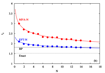
Figure 1: (a) Schematic representation of the honeycomb lattice (b) the variation of the critical temperature with the size of the cluster, for the honeycomb lattice. Exact result ($1.519$) [25] and the result of the BPA ($1.821$) [26] also shown as horizontal lines. Results are shown by points and also fitted curve of the form $aN^{-b}$ depicted both of the methods MFA-$N$ and EFT-$N$.

Table 1: Number of elements in configuration set $\{t_{k}\}$ for Eq. (47), for the honeycomb ($z=3$), square ($z=4$) and simple cubic ($z=6$) lattices.

$N$	$z=3$	$z=4$	$z=6$
$1$	$4$	$5$	$7$
$2$	$9$	$16$	$36$
$3$	$18$	$48$	$180$
$4$	$36$	$81$	$625$
$5$	$72$	$216$	$3000$
$6$	$64$	$324$	$10000$
$7$	$96$	$864$	$32000$
$8$	$192$	$972$	$65536$

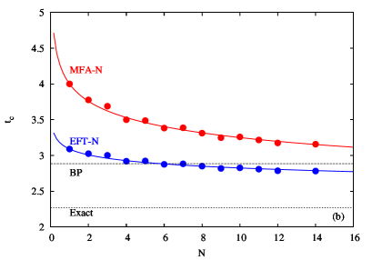
Figure 2: (a) Schematic representation of the square lattice (b) the variation of the critical temperature with the size of the cluster, for the square lattice. Exact result ($2.269$) [27] and the result of the BPA ($2.885$) [26] also shown as horizontal lines. Results are shown by points and also fitted curve of the form $aN^{-b}$ depicted for both of the methods MFA-$N$ and EFT-$N$.

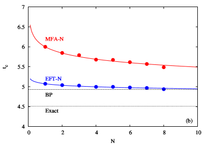
Figure 3: (a) Schematic representation of the simple cubic lattice (b) the variation of the critical temperature with the size of the cluster, for the simple cubic lattice. Exact result ($4.511$) [25] and the result of the BPA ($4.933$) [26] also shown as horizontal lines. Results are shown by points and also fitted curve of the form $aN^{-b}$ depicted both of the methods MFA-$N$ and EFT-$N$.

Table 2: $t_{c}=aN^{-b}$ least squares fitting results for the MFT-$N$ formulation

Lattice ($z$)	$b$	Sum of squares of residuals	$N_{BP}$	$N_{exact}$
$3$	$0.1262$	$0.0110$	$52$	$217$
$4$	$0.0901$	$0.0095$	$37$	$537$
$6$	$0.0384$	$0.0055$	$164$	$1691$

Table 3: $t_{c}=aN^{-b}$ least squares fitting results for the EFT-$N$ formulation

Lattice ($z$)	$b$	Sum of Squares of residuals	$N_{BP}$	$N_{exact}$
$3$	$0.0584$	$0.0034$	$12$	$259$
$4$	$0.0389$	$0.0036$	$6$	$2868$
$6$	$0.0108$	$0.0009$	$13$	$51478$

As explained above, enlarging the cluster yields more accurate results for the critical temperatures. But on some problems we have to use larger clusters, even though we do not need the more accurate results. Both of the approximations in $1$-spin cluster cannot distinguish of some different lattice types. Most trivial example is EFT-$1$ formulation can not distinguish the simple cubic lattice from the triangular lattice, since both of the lattices have coordination number (number of nearest neighbors) 6 and EFT-$1$ uses only the coordination numbers. This deficiency may yield some dramatic results. In order to explain this point, suppose that we have a magnetic system with a geometry given as Fig. (4). System is infinitely long about the $z$ axis and finite in $xy$ plane. With this geometry we can model the single walled nanotube. In this form there are number of 6 spins in each plane. Beside the present interaction between this nearest neighbor spins in one plane, also there are interactions with nearest neighbor spins in the lower and upper planes. Let us call $L=6$ as the size of the nanotube, which is the number of spins in each $xy$ plane. While in Fig. (4) the size of the nanotube is 6, there can exist bigger or lower sizes. For instance $L=3$ is a three-leg spin tube [28]. Regardless of the size of the nanotube, if we solve this system with EFT-$1$, we obtain the results of the square lattice. Because of Eq. (26) (or Eq. (30)) contains only the coordination number as a representation of the geometry of the system. Then we have to enlarge the cluster. One of the reasonable choice is to construct a finite cluster from the $L$ spins, which are in the same plane. We can see the results for the critical temperatures for this system in Fig. (5). Constructed cluster sizes and the size of the nanotube are the same, i.e. results taken from the $L$-spin cluster, where the cluster consists of the spins that belong to the one plane of the system. MFA-$1$ and EFT-$1$ results have been shown by horizontal lines in Fig. (5) with the values $t_{c}=4.000$ and , $t_{c}=3.090$ respectively. As seen in Fig. (5), critical temperature rises when the size of the nanotube gets bigger, as physically expected. But as seen in Fig. (5), 1-spin cluster formulations cannot give this situation.

Lastly, EFRG calculations on S-1/2 Ising systems can be easily done by using Eq. (47). As an example of this, we have depicted the variation of the critical temperature of the square lattice (obtained within the EFRG formulation) with some selected cluster sizes in Fig. 6. As seen in Fig. 6 that, critical temperatures obtained from both of the methods (namely, EFRG and MFRG) approach to the exact result, while the size of the clusters rise. Results for MFRG-$(2,1)$ ($t_{c}=2.885$), EFRG-$(2,1)$ ($t_{c}=2.794$) are the same as given in Refs. [29] and [22], respectively. On the other hand, the results of EFRG-$(9,8)$ ($t_{c}=2.450$) and EFRG-$(12,11)$ ($t_{c}=2.408$) are lower than the obtained value of EFRG-$(9,6)$ ($t_{c}=2.572$) in Ref. [23]. To the best of our knowledge, these last two results have not been obtained within the EFRG yet.

Figure 4: Schematic representation of the single-walled nanotube with size $L=6$.

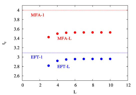
Figure 5: Variation of the critical temperature of the single-walled nanotube with the size of the nanotube, for both formulations MFA-$L$ and EFT- $L$. The results of the MFA-$1$ and EFT- $1$ also shown with horizontal lines.

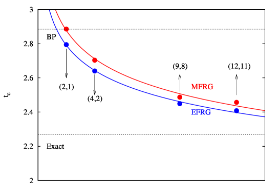
Figure 6: Critical temperatures of the S-1/2 Ising model on square lattice obtained from EFRG and MFRG methods. Cluster sizes that used in both methods shown in parenthesis. The horizontal lines named as BP and Exact are the results of BPA and exact calculations.

4.2 Thermodynamic Properties

In this section we want to investigate the effect of the enlarging the cluster on the thermodynamic properties of the system. Since different lattices have similar behaviors then we restrict ourselves in only square lattice.

Magnetization can be calculated from Eq. (44) as explained in Sec. 3. The differentiation of Eq. (44) with respect to magnetic field will give the magnetic susceptibility ($\chi$) of the system. Besides, internal energy of the system (denoted as $u$, which is scaled by $J$) can be calculated as the same way of magnetization. The only difference is the starting point of the calculation i.e. in Eq. (8), instead of $S_{k}$ there will be terms like $S_{k}S_{l}$ which are the nearest neighbors of the chosen cluster. Again, differentiation of this expression with respect to the temperature will give the specific heat (denoted by $c$, which is again scaled by $J$).

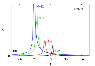
Figure 7: Variation of the (a) zero-field magnetization and (b) zero-field magnetic susceptibility of the S-1/2 Ising model on a square lattice, with the formulation EFT-$N$ and for selected values of cluster sizes, $N=2,4,9,12$.

In order to see the effect of the enlarging cluster within the EFT-$N$ formulation, we depict the variation of the magnetization and the magnetic susceptibility of the system at zero magnetic field, with the temperature for different cluster sizes in Fig. 7. As seen in Fig. 7 (a) the magnetization behaviors with the temperature are the same for all of the clusters. The only difference comes from the critical temperature, in which the magnetization reaches to value of zero. As the size of the cluster increases, the critical temperature decreases, as shown also in Fig. 2 (b). This decreasing behavior of the critical temperature shows itself also in the behavior of the magnetic susceptibility. As seen in Fig. 7 (b), while the size of the cluster increases, the peaks of the susceptibility curves grow as well as they shift to the right of the $(\chi-t)$ plane, i.e. lower temperature regions. As we can see from 7 (b) that, enlarging cluster gives more realistic results for the magnetic susceptibility, since the divergence behavior of the magnetic susceptibility at a critical temperature appears more strongly as the size of the cluster rises.

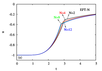
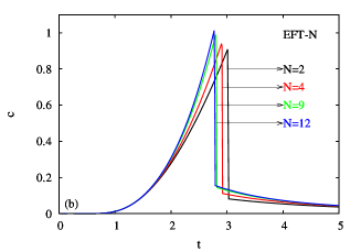
Figure 8: Variation of the (a) internal energy and (b) specific heat of the S-1/2 Ising model on a square lattice, with the formulation EFT-$N$ and for selected values of cluster sizes, $N=2,4,9,12$.

We can make similar conclusions about the behavior of the internal energy and the specific heat of the system, when the size of the cluster rises within the EFT-$N$ formulation. We can see from Fig. 8 (a) that, the change in the behavior of the internal energy with temperature, occurs at lower values of the temperature as the cluster size rises, since enlarging cluster causes to decline of the critical temperature. The same thing shows itself in Fig. 8 (b) also, which is the variation of the specific heat with the temperature for some selected values of the cluster sizes. The peaks, which occurs at the critical temperature, getting higher when the cluster size rises.

All these comments suggest that, within the EFT-$N$ formulation, enlarging the cluster also will give more realistic results in the thermodynamic properties of the system. As in the effect of the enlarging cluster on the critical temperatures of the system, while rising the size of the cluster, the difference between the successive curves getting smaller.

5 Conclusion

In conclusion, a general formulation for the EFT with differential operator technique and DA (as well as MFT) with larger finite clusters has been derived. Enlarging the finite cluster yields different formulations which are called EFT-$N$ (or MFT-$N$) for the $N$-spin cluster. The formulation is limited to the S-1/2 Ising model on completely translationally invariant lattices.

It has been shown that, application of the EFT-$N$ and MFT-$N$ formulations on several lattices yield more accurate results in critical temperatures as well as the thermodynamic properties of the system, when the size of the cluster rises. Comparisons of the results in the critical temperatures have been made with the results of the BPA and exact ones. It has been shown that EFT-$6$ and MFT-$37$ results and EFT-$13$ and MFT-$164$ results in the critical temperature, gives the results of the BPA for the square and simple cubic lattices, respectively. We note here that, constructing process of the finite cluster with $N$ spins can be made in several ways. Different geometrical clusters which have the same number of spins will give different results.

Besides, the limitations of the derived formulation have been discussed, since enlarging the cluster yield more and more numerical computations, and then takes more and more time. Anyway, we can say that the formulation derived in this work can be applied to any cluster size, in principle.

Besides all of these, derived formulation can be used in EFRG (and MFRG) formulations. The effect of the enlarging cluster on the critical temperatures of the square lattice within EFRG formulation has been also discussed, with applying the formulation. The simplest possible MFRG formulation gives the results of the BPA in the critical temperature, while the EFRG results lie always below of the MFRG results, as expected.

In addition to all of these observations, necessity of the using $N$-spin cluster formulations in some systems (such as nano magnetic systems) has been discussed. Constructing EFT-$N$ formulation for the magnetic nano materials will be the topic of the future work.

We hope that the results obtained in this work may be beneficial form both theoretical and experimental point of view.

References

- [1] R. J. Baxter, Exactly Solved Models in Statistical Mechanics (London: Academic Press, 1982).
- [2] E. Ising, Zeitschrift für Physik, 31, (1925) 253.
- [3] L. Onsager, Phys. Rev. 65, 117 (1944)
- [4] J. S. Smart, Effective Field Theories of Magnetism, Saunders, London, 1966.
- [5] S. Mukhopadhyay, I. Chatterjee, Journal of Magnetism and Magnetic Materials 270 (2004) 247
- [6] T. Oguchi, Progr. Theoret. Phys. (Kyoto) 13 (1955) 148.
- [7] H. A. Bethe, Proc. Roy. Soc., London A 150 (1935) 552.
- [8] R. F. Peierls, Proc. Canbridge Phil. Soc. 32 (1936) 477.
- [9] H. B. Callen, Phys. Lett. 4 (1963) 161.
- [10] M. Suzuki, Phys. Lett. 19 (1965) 267.
- [11] R. Honmura, T. Kaneyoshi, J. Phys. C 12 (1979) 3979.
- [12] T. Kaneyoshi, Acta Phys. Pol. A 83 (1993) 703.
- [13] F. Zernike, Physica 7 (1940) 565.
- [14] N. Matsudaira, J. Phys. Soc. Japan 35 (1973) 1593.
- [15] N. Boccara, Phys. Lett. A 94 (1983) 185.
- [16] T. Balcerzak, J. Magn. Magn. Mater. 97, 152 (1991).
- [17] M. Saber, Chin. J. Phys. 35 (1997) 577.
- [18] A. Bobák, M. Jaščur Phys. Stat. Sol. B 135, (1986) K9.
- [19] O. R. Salmon , J. R. de Sousa and F. D. Nobre Physics Letters A 373 (2009) 2525
- [20] J.O. Indekeu, A. Maritan, A.C. Stella, J. Phys. A 15 (1982) L291.
- [21] V. Ilkovič, Phys. Stat. Sol. (B), 166 (1991) K31.
- [22] I.P. Fittipaldi, D.F. de Albuquerque, J. Magn. Magn. Mater. 107 (1992) 236.
- [23] D.F. de Albuquerque, E. Santos-Silva, N.O. Moreno J. Magn. Magn. Mater. L63 (2009) 321.
- [24] Ü. Akıncı arXiv:1308.2511v2 (2014).
- [25] M.E. Fisher, Rep. Prog. Phys. 30, (1967) 615.
- [26] T. Kaneyoshi, Physica A 269, (1999) 344.
- [27] L. Onsager, Phys. Rev. 65, (1944) 197.
- [28] T. Sakai, M. Sato , K. Okamoto, K. Okunishi and C. Itoi J. Phys.: Condens. Matter 22 (2010) 403201
- [29] J.O. Indekeu, A. Martian, A.L. Stella, Phys. Rev. B 35 (1987) 305.