A multilevel Monte Carlo method for computing failure probabilities

Abstract

We propose and analyze a method for computing failure probabilities of systems modeled as numerical deterministic models (e.g., PDEs) with uncertain input data. A failure occurs when a functional of the solution to the model is below (or above) some critical value. By combining recent results on quantile estimation and the multilevel Monte Carlo method we develop a method which reduces computational cost without loss of accuracy. We show how the computational cost of the method relates to error tolerance of the failure probability. For a wide and common class of problems, the computational cost is asymptotically proportional to solving a single accurate realization of the numerical model, i.e., independent of the number of samples. Significant reductions in computational cost are also observed in numerical experiments.

1 Introduction

This paper is concerned with the computational problem of finding the probability for failures of a modeled system. The model input is subject to uncertainty with known distribution and a failure is the event that a functional (quantity of interest, QoI) of the model output is below (or above) some critical value. The goal of this paper is to develop an efficient and accurate multilevel Monte Carlo (MLMC) method to find the failure probability. We focus mainly on the case when the model is a partial differential equation (PDE) and we use terminology from the discipline of numerical methods for PDEs. However, the methodology presented here is also applicable in a more general setting.

A multilevel Monte Carlo method inherits the non-intrusive and non-parametric characteristics from the standard Monte Carlo (MC) method. This allows the method to be used for complex black-box problems for which intrusive analysis is difficult or impossible. The MLMC method uses a hierarchy of numerical approximations on different accuracy levels. The levels in the hierarchy are typically directly related to a grid size or timestep length. The key idea behind the MLMC method is to use low accuracy solutions as control variates for high accuracy solutions in order to construct an estimator with lower variance. Savings in computational cost are achieved when the low accuracy solutions are cheap and are sufficiently correlated with the high accuracy solutions. MLMC was first introduced in [8] for stochastic differential equations as a generalization of a two-level variance reduction technique introduced in [15]. The method has been applied to and analyzed for elliptic PDEs in [3, 2, 17]. Further improvements of the MLMC method, such as work on optimal hierarchies, non-uniform meshes and more accurate error estimates can be found in [13, 4]. In the present paper, we are not interested in the expected value of the QoI, but instead a failure probability, which is essentially a single point evaluation of the cumulative distribution function (cdf). For extreme failure probabilities, related methods include importance sampling [12], importance splitting [11], and subset simulations [1]. Works more related to the present paper include non-parameteric density estimation for PDE models in [7], and in particular [6]. In the latter, the selective refinement method for quantiles was formulated and analyzed.

In this paper, we seek to compute the cdf at a given critical value. The cdf at the critical value can be expressed as the expectation value of a binomially distributed random variable $Q$ that is equal to $1$ if the QoI is smaller than the critical value, and $0$ otherwise. The key idea behind selective refinement is that realizations with QoI far from the critical value can be solved to a lower accuracy than those close to the critical value, and still yield the same value of $Q$. The random variable $Q$ lacks regularity with respect to the uncertain input data, and hence we are in an unfavorable situation for application of the MLMC method. However, with the computational savings from the selective refinement it is still possible to obtain an asymptotic result for the computational cost where the cost for the full estimator is proportional to the cost for a single realization to the highest accuracy.

The paper is structured as follows. Section 2 presents the necessary assumptions and the precise problem description. It is followed by Section 3 where our particular failure probability functional is defined and analyzed for the MLMC method. In Section 4 and Section 5 we revisit the multilevel Monte Carlo and selective refinement method adapted to this problem and in Section 6 we show how to combine multilevel Monte Carlo with the selective refinement to obtain optimal computational cost. In Section 7 we give details on how to implement the method in practice. The paper is concluded with two numerical experiments in Section 8.

2 Problem formulation

We consider a model problem $\mathcal{M}$, e.g., a (non-)linear differential operator with uncertain data. We let $u$ denote the solution to the model

$$\mathcal{M}(\omega,u)=0,$$

where the data $\omega$ is sampled from a space $\Omega$. In what follows we assume that there exists a unique solution $u$ given any $\omega\in\Omega$ almost surely. It follows that the solution $u$ to a given model problem $\mathcal{M}$ is a random variable which can be parameterized in $\omega$, i.e., $u=u(\omega)$.

The focus of this work is to compute failure probabilities, i.e., we are not interested in some pointwise estimate of the expected value of the solution, $\mathbb{E}\mathopen{}\mathclose{{}\left[u}\right]$, but rather the probability that a given QoI expressed as a functional, $X(u)$ of the solution $u$, is less (or greater) than some given critical value $y$. We let $F$ denote the cdf of the random variable $X=X(\omega)$. The failure probability is then given by

$$p=F(y)=\Pr(X\leq y).$$ (1)

The following example illustrates how the problem description relates to real world problems.

Example 1.

As an example, geological sequestration of carbon dioxide (CO_2) is performed by injection of CO_2 in an underground reservoir. The fate of the CO_2 determines the success or failure of the storage system. The CO_2 propagation is often modeled as a PDE with random input data, such as a random permeability field. Typical QoIs include reservoir breakthrough time or pressure at a fault. The value $y$ corresponds to a critical value which the QoI may not exceed or go below. In the breakthrough time case, low values are considered failure. In the pressure case, high values are considered failure. In that case one should negate the QoI to transform the problem to the form of equation (1).

The only regularity assumption on the model is the following Lipschitz continuity assumption of the cdf, which is assumed to hold throughout the paper.

Assumption 2.

For any $x,y\in\mathbb{R}$,

$$|F(x)-F(y)|\leq C_{L}|x-y|.$$ (2)

To compute the failure probability we consider the binomially distributed variable $Q=\mathbbm{1}{(X\leq y)}$ which takes the value $1$ if $X\leq y$ and $0$ otherwise. The cdf can be expressed as the expected value of $Q$, i.e., $p=F(y)=\mathbb{E}\mathopen{}\mathclose{{}\left[Q}\right]$. In practice we construct an estimator $\widehat{Q}$ for $\mathbb{E}\mathopen{}\mathclose{{}\left[Q}\right]$, based on approximate sample values from $X$. As such, $\widehat{Q}$ often suffers from numerical bias from the approximation in the underlying sample. Our goal is to compute the estimator $\widehat{Q}$ to a given root mean square error (RMSE) tolerance $\epsilon$, i.e., to compute

$$e\mathopen{}\mathclose{{}\left[\widehat{Q}}\right]=\mathopen{}\mathclose{{}\left(\mathbb{E}\mathopen{}\mathclose{{}\left[\mathopen{}\mathclose{{}\left(\widehat{Q}-\mathbb{E}\mathopen{}\mathclose{{}\left[Q}\right]}\right)^{2}}\right]}\right)^{1/2}=\mathopen{}\mathclose{{}\left(\mathbb{V}\mathopen{}\mathclose{{}\left[\widehat{Q}}\right]+\mathopen{}\mathclose{{}\left(\mathbb{E}\mathopen{}\mathclose{{}\left[\widehat{Q}-Q}\right]}\right)^{2}}\right)^{1/2}\leq\epsilon$$

to a minimal computational cost. The equality above shows a standard way of splitting the RMSE into a stochastic error and numerical bias contribution.

The next section presents assumptions and results regarding the numerical discretization of the particular failure probability functional $Q$.

3 Approximate failure probability functional

We will not consider a particular approximation technique for computing $\widehat{Q}$, but instead make some abstract assumptions on the underlying discretization. We introduce a hierarchy of refinement levels $\ell=0,1,\ldots$ and let $X^{\prime}_{\ell}$ and $Q^{\prime}_{\ell}=\mathbbm{1}{(X^{\prime}_{\ell}\leq y)}$ be an approximate QoI of the model, and approximate failure probability, respectively, on level $\ell$. One possible and natural way to define the accuracy on level $\ell$ is by assuming

$$\mathopen{}\mathclose{{}\left|X-X^{\prime}_{\ell}}\right|\leq\gamma^{\ell},$$ (3)

for some $0<\gamma<1$. This means the error of all realizations on level $\ell$ are uniformly bounded by $\gamma^{\ell}$. In a PDE setting, typically an a priori error bound or a posteriori error estimate,

$$\mathopen{}\mathclose{{}\left|X(\omega)-X_{h}(\omega)}\right|\leq C(\omega)h^{s},$$

can be derived for some constants $C(\omega)$, $s$, and a discretization parameter $h$. Then we can choose $X^{\prime}_{\ell}=X_{h}$ with $h=\mathopen{}\mathclose{{}\left(C(\omega)^{-1}\gamma^{\ell}}\right)^{1/s}$ to fulfill (3).

For an accurate value of the failure probability functional the condition in (3) is unnecessarily strong. This functional is very sensitive to perturbations of values close to $y$, but insensitive to perturbations for values far from $y$. This insensitivity can be exploited. We introduce a different approximation $X_{\ell}$, and impose the following, relaxed, assumption on this approximation of $X$, which allows for larger errors far from the critical value $y$. This assumption is illustrated in Figure 1.

Assumption 3.

The numerical approximation $X_{\ell}$ of $X$ satisfies

$$\mathopen{}\mathclose{{}\left|X-X_{\ell}}\right|\leq\gamma^{\ell}\quad\text{ or }\quad\mathopen{}\mathclose{{}\left|X-X_{\ell}}\right|<\mathopen{}\mathclose{{}\left|X_{\ell}-y}\right|$$ (4)

for a fix $0<\gamma<1$.

Figure 1: Illustration of condition (4). The numerical error is allowed to be larger than $\gamma^{\ell}$ far away from $y$.

We define $Q_{\ell}=\mathbbm{1}{(X_{\ell}\leq y)}$ analogously to $Q^{\prime}_{\ell}$. Let us compare the implications of the two conditions (3) and (4) on the quality of the two respective approximations. Denote by $X^{\prime}_{\ell}$ and $Q^{\prime}_{\ell}$ stochastic variables obeying the error bound (3) and its corresponding approximate failure functional, respectively, and let $X_{\ell}$ obey (4). In a practical situation, Assumption 3 is fulfilled by iterative refinements of $X_{\ell}$ until condition (4) is satisfied. It is natural to use a similar procedure to achieve the stricter condition (3) for $X^{\prime}_{\ell}$. We express this latter assumption of using similar procedures for computing $X_{\ell}$ and $X^{\prime}_{\ell}$ as

$$|X-X_{\ell}|\leq\gamma^{\ell}\text{ implies }X^{\prime}_{\ell}=X_{\ell},$$ (5)

i.e., for outcomes where $X_{\ell}$ is solved to accuracy $\gamma^{\ell}$, $X^{\prime}_{\ell}$ is equal to $X_{\ell}$. Under that assumption, the following lemma shows that it is not less probable that $Q_{\ell}$ is correct than that $Q^{\prime}_{\ell}$ is.

Lemma 4.

Let $X^{\prime}_{\ell}$ and $X_{\ell}$ fulfill (3) and (4), respectively, and assume (5) holds. Then $\Pr(Q_{\ell}=Q)\geq\Pr(Q^{\prime}_{\ell}=Q)$.

Proof.

We split $\Omega$ into the events $A=\{\omega\in\Omega:|X-X_{\ell}|\leq\gamma^{\ell}\}$ and its complement $\Omega\setminus A$. For $\omega\in A$, using (5), we conclude that $Q^{\prime}_{\ell}=Q_{\ell}$, hence

$$\Pr(Q_{\ell}=Q\;|\;A)=\Pr(Q^{\prime}_{\ell}=Q\;|\;A).$$

For $\omega\notin A$, we have $|X-X_{\ell}|>\gamma^{\ell}$, and from (4) that $|X-X_{\ell}|<|X_{\ell}-y|$, i.e., $Q_{\ell}=Q$ and hence

$$\Pr(Q_{\ell}=Q\;|\;\Omega\setminus A)=1.$$

Since $\Pr(Q^{\prime}_{\ell}=Q\;|\;\Omega\setminus A)\leq 1$, we get $\Pr(Q_{\ell}=Q)\geq\Pr(Q^{\prime}_{\ell}=Q)$. ∎

Under Assumption 3 we can prove the following lemma on the accuracy of the failure probability function $Q_{\ell}$.

Lemma 5.

Under Assumption 2 and 3, the statements

M1

$\mathopen{}\mathclose{{}\left|\mathbb{E}\mathopen{}\mathclose{{}\left[Q_{\ell}-Q}\right]}\right|\leq C_{1}\gamma^{\ell}$,

M2

$\mathbb{V}\mathopen{}\mathclose{{}\left[Q_{\ell}-Q_{\ell-1}}\right]\leq C_{2}\gamma^{\ell}$ for $\ell\geq 1$,

are satisfied where $C_{1}$ and $C_{2}$ do not depend on $\ell$.

Proof.

We split $\Omega$ into the events $B=\{\omega\in\Omega:\gamma^{\ell}\geq|X_{\ell}-y|\}$ and its complement $\Omega\setminus B$. In $\Omega\setminus B$, we have $Q_{\ell}=Q$, since $|X-X_{\ell}|<|X_{\ell}-y|$ from (4). Also, we note that the event $B$ implies $|X-X_{\ell}|\leq\gamma^{\ell}$, hence $|X-y|\leq 2\gamma^{\ell}$. Then,

$$|\mathbb{E}\mathopen{}\mathclose{{}\left[Q_{\ell}-Q}\right]| =\mathopen{}\mathclose{{}\left|\int_{B}Q_{\ell}(\omega)-Q(\omega)\,\mathrm{d}P(\omega)}\right|\leq\int_{B}1\,\mathrm{d}P(\omega)$$

$$\leq\Pr(|X-y|\leq 2\gamma^{\ell})=F(y-2\gamma^{\ell})-F(y+2\gamma^{\ell})$$

$$\leq 4C_{L}\gamma^{\ell},$$

which proves M1. M2 follows directly from M1, since

$$\mathbb{V}\mathopen{}\mathclose{{}\left[Q_{\ell}-Q_{\ell-1}}\right] =\mathbb{E}\mathopen{}\mathclose{{}\left[(Q_{\ell}-Q_{\ell-1})^{2}}\right]-\mathbb{E}\mathopen{}\mathclose{{}\left[Q_{\ell}-Q_{\ell-1}}\right]^{2}$$

$$\leq\mathbb{E}\mathopen{}\mathclose{{}\left[Q_{\ell}-2Q_{\ell}Q_{\ell-1}+Q_{\ell-1}}\right]$$

$$\leq\mathopen{}\mathclose{{}\left|\mathbb{E}\mathopen{}\mathclose{{}\left[Q_{\ell}-Q}\right]}\right|+\mathopen{}\mathclose{{}\left|2\mathbb{E}\mathopen{}\mathclose{{}\left[Q_{\ell}Q_{\ell-1}-Q}\right]}\right|+\mathopen{}\mathclose{{}\left|\mathbb{E}\mathopen{}\mathclose{{}\left[Q_{\ell-1}-Q}\right]}\right|$$

$$\leq 2\mathopen{}\mathclose{{}\left|\mathbb{E}\mathopen{}\mathclose{{}\left[Q_{\ell}-Q}\right]}\right|+2\mathopen{}\mathclose{{}\left|\mathbb{E}\mathopen{}\mathclose{{}\left[Q_{\ell-1}-Q}\right]}\right|$$

$$\leq C_{2}\gamma^{\ell},$$

where $(Q_{\ell})^{2}=Q_{\ell}$ was used. ∎

Interesting to note with this particular failure probability functional is that the convergence rate in M2 cannot be improved if the rate in M1 is already sharp, as the following lemma shows.

Lemma 6.

Let $0<\gamma<1$ be fixed. If there is a $0<c\leq 1$ such that the failure probability functional satisfies

$$c\gamma^{\ell}\leq|\mathbb{E}\mathopen{}\mathclose{{}\left[Q_{\ell}-Q}\right]|\leq C_{1}\gamma^{\ell}$$

for all $\ell=0,\ldots$, then

$$\mathbb{V}\mathopen{}\mathclose{{}\left[Q_{\ell}-Q_{\ell-1}}\right]\leq C_{2}\gamma^{\beta\ell},$$

where $\beta=1$ is sharp in the sense that the relation will be violated for sufficiently large $\ell$, if $\beta>1$.

Proof.

Assume that $\mathbb{V}\mathopen{}\mathclose{{}\left[Q_{\ell}-Q_{\ell-1}}\right]\leq C\gamma^{\beta\ell}$ for for some constant $C$ and $\beta>1$. For two levels $\ell$ and $k$, we have that

$$|\mathbb{E}\mathopen{}\mathclose{{}\left[Q_{\ell}-Q_{k}}\right]| \geq\mathopen{}\mathclose{{}\left||\mathbb{E}\mathopen{}\mathclose{{}\left[Q_{\ell}-Q}\right]|-|\mathbb{E}\mathopen{}\mathclose{{}\left[Q_{k}-Q}\right]|}\right|\geq\mathopen{}\mathclose{{}\left(c-\gamma^{\ell-k}}\right)\gamma^{k}.$$

Choosing $\ell$ and $k$ such that $\ell>k$ and $c-\gamma^{\ell-k}>0$ yields

$$\mathopen{}\mathclose{{}\left(c-\gamma^{\ell-k}}\right)\gamma^{k} \leq|\mathbb{E}\mathopen{}\mathclose{{}\left[Q_{\ell}-Q_{k}}\right]|\leq\sum_{j=k}^{\ell-1}|\mathbb{E}\mathopen{}\mathclose{{}\left[Q_{j+1}-Q_{j}}\right]|\leq\sum_{j=k}^{\ell-1}\mathbb{E}\mathopen{}\mathclose{{}\left[(Q_{j+1}-Q_{j})^{2}}\right]$$

$$=\sum_{j=k}^{\ell-1}\mathopen{}\mathclose{{}\left(\mathbb{V}\mathopen{}\mathclose{{}\left[Q_{j+1}-Q_{j}}\right]+\mathopen{}\mathclose{{}\left(\mathbb{E}\mathopen{}\mathclose{{}\left[Q_{j+1}-Q_{j}}\right]}\right)^{2}}\right)$$

$$\leq\sum_{j=k}^{\ell-1}\mathopen{}\mathclose{{}\left(C\gamma^{\beta j}+\mathcal{O}(\gamma^{2j})}\right)\leq\widetilde{C}\gamma^{\beta k}+\mathcal{O}(\gamma^{2k}).$$

For $\ell,k\to\infty$ we have a contradiction and hence $\beta\leq 1$, which proves that the bound can not be improved. ∎

4 Multilevel Monte Carlo method

In this section, we present the multilevel Monte Carlo method in a general context. Because of the low convergence rate of the variance in M2, the MLMC method does not perform optimally for the failure probability functional. The results presented here will be combined with the results from Section 5 to derive a new method to compute failure probabilities efficiently in Section 6.

The (standard) MC estimator at refinement level $\ell$ of $\mathbb{E}\mathopen{}\mathclose{{}\left[Q}\right]$ using a sample $\{\omega^{i}_{\ell}\}_{i=1}^{N_{\ell}}$, reads

$$\widehat{Q}^{MC}_{N_{\ell},\ell}=\frac{1}{N_{\ell}}\sum_{i=1}^{N_{\ell}}Q_{\ell}(\omega^{i}_{\ell}).$$

Note that the subscripts $N_{\ell}$ and $\ell$ control the statistical error and numerical bias, respectively. The expected value and variance of the estimator $\widehat{Q}^{MC}_{N_{\ell},\ell}$ are $\mathbb{E}\mathopen{}\mathclose{{}\left[\widehat{Q}^{MC}_{N_{\ell},\ell}}\right]=\mathbb{E}\mathopen{}\mathclose{{}\left[Q_{\ell}}\right]$ and $\mathbb{V}\mathopen{}\mathclose{{}\left[\widehat{Q}^{MC}_{N_{\ell},\ell}}\right]=N_{\ell}^{-1}\mathbb{V}\mathopen{}\mathclose{{}\left[Q_{\ell}}\right]$, respectively. Referring to the goal of the paper, we want the MSE (square of the RMSE) to satisfy

$$e\mathopen{}\mathclose{{}\left[\widehat{Q}^{MC}_{N_{\ell},\ell}}\right]^{2}=N_{\ell}^{-1}\mathbb{V}\mathopen{}\mathclose{{}\left[Q_{\ell}}\right]+\mathopen{}\mathclose{{}\left(\mathbb{E}\mathopen{}\mathclose{{}\left[Q_{\ell}-Q}\right]}\right)^{2}\leq\epsilon^{2}/2+\epsilon^{2}/2=\epsilon^{2},$$

i.e., both the statistical error and the numerical error should be less than $\epsilon^{2}/2$. The MLMC method is a variance reduction technique for the MC method. The MLMC estimator $\widehat{Q}^{ML}_{\{N_{\ell}\},L}$ at refinement level $L$ is expressed as a telescoping sum of $L$ MC estimator correctors:

$$\widehat{Q}^{ML}_{\{N_{\ell}\},L}=\sum_{\ell=0}^{L}\frac{1}{N_{\ell}}\sum_{i=1}^{N_{\ell}}\mathopen{}\mathclose{{}\left(Q_{\ell}(\omega^{i}_{\ell})-Q_{\ell-1}(\omega^{i}_{\ell})}\right),$$

where $Q_{-1}=0$. There is one corrector for every refinement level $\ell=0,\ldots,L$, each with a specific MC estimator sample size $N_{\ell}$. The expected value and variance of the MLMC estimator are

$$\mathbb{E}\mathopen{}\mathclose{{}\left[\widehat{Q}^{ML}_{\{N_{\ell}\},L}}\right] =\sum_{\ell=0}^{L}\mathbb{E}\mathopen{}\mathclose{{}\left[Q_{\ell}-Q_{\ell-1}}\right]=\mathbb{E}\mathopen{}\mathclose{{}\left[Q_{L}}\right]\quad\text{and}$$ (6)

$$\mathbb{V}\mathopen{}\mathclose{{}\left[\widehat{Q}^{ML}_{\{N_{\ell}\},L}}\right] =\sum_{\ell=0}^{L}N_{\ell}^{-1}\mathbb{V}\mathopen{}\mathclose{{}\left[Q_{\ell}-Q_{\ell-1}}\right],$$

respectively. Using (6) the MSE for the MLMC estimator can be expressed as

$$e\mathopen{}\mathclose{{}\left[\widehat{Q}^{ML}_{\{N_{\ell}\},L}}\right]^{2} =\sum_{\ell=0}^{L}N_{\ell}^{-1}\mathbb{V}\mathopen{}\mathclose{{}\left[Q_{\ell}-Q_{\ell-1}}\right]+\mathopen{}\mathclose{{}\left(\mathbb{E}\mathopen{}\mathclose{{}\left[Q_{L}-Q}\right]}\right)^{2},$$

and can be computed at expected cost

$$\mathcal{C}\mathopen{}\mathclose{{}\left[\widehat{Q}^{ML}_{\{N_{\ell}\},L}}\right]=\sum_{\ell=0}^{L}N_{\ell}c_{\ell},$$

where $c_{\ell}=\mathcal{C}\mathopen{}\mathclose{{}\left[Q_{\ell}}\right]+\mathcal{C}\mathopen{}\mathclose{{}\left[Q_{\ell-1}}\right]$. Here, by $\mathcal{C}\mathopen{}\mathclose{{}\left[\cdot}\right]$ we denote the expected computational cost to compute a certain quantity. Given that the variance of the MLMC estimator is $\epsilon^{2}/2$ the expected cost is minimized by choosing

$$N_{\ell}=2\epsilon^{-2}\sqrt{\mathbb{V}\mathopen{}\mathclose{{}\left[Q_{\ell}-Q_{\ell-1}}\right]/c_{\ell}}\sum_{k=0}^{L}\sqrt{\mathbb{V}\mathopen{}\mathclose{{}\left[Q_{k}-Q_{k-1}}\right]c_{k}}$$ (7)

(see Appendix A), and hence the total expected cost is

$$\mathcal{C}\mathopen{}\mathclose{{}\left[\widehat{Q}^{ML}_{\{N_{\ell}\},L}}\right]=2\epsilon^{-2}\mathopen{}\mathclose{{}\left(\sum_{\ell=0}^{L}\sqrt{\mathbb{V}\mathopen{}\mathclose{{}\left[Q_{\ell}-Q_{\ell-1}}\right]c_{\ell}}}\right)^{2}.$$ (8)

If the product $\mathbb{V}\mathopen{}\mathclose{{}\left[Q_{\ell}-Q_{\ell-1}}\right]c_{\ell}$ increases (or decreases) with $\ell$ then dominating term in (8) will be $\ell=L$ (or $\ell=0$). The values $N_{\ell}$ can be estimated on the fly in the MLMC algorithm using (7) while the cost $c_{\ell}$ can be estimated using an a priori model. The computational complexity to obtain a RMSE less than $\epsilon$ of the MLMC estimator for the failure probability functional is given by the theorem below. In the following, the notation $a\lesssim b$ stands for $a\leq Cb$ with some constant $C$ independent of $\epsilon$ and $\ell$.

Theorem 7.

Let Assumption 2 and 3 hold (so that Lemma 5 holds) and $\mathcal{C}\mathopen{}\mathclose{{}\left[Q_{\ell}}\right]\lesssim\gamma^{-r\ell}$. Then there exists a constant $L$ and a sequence $\{N_{\ell}\}$ such that the RMSE is less than $\epsilon$, and the expected cost of the MLMC estimator is

$$\mathcal{C}\mathopen{}\mathclose{{}\left[\widehat{Q}^{ML}_{\{N_{\ell}\},L}}\right]\lesssim\begin{cases}\epsilon^{-2}&\quad r<1\\ \epsilon^{-2}(\log\epsilon^{-1})^{2}&\quad r=1\\ \epsilon^{-1-r}&\quad r>1.\\ \end{cases}$$ (9)

Proof.

For a proof see, e.g., [3, 8]. ∎

The most straight-forward procedure to fulfill Assumption 3 in practice is to refine all samples on level $\ell$ uniformly to an error tolerance $\gamma^{\ell}$, i.e., to compute $X^{\prime}_{\ell}$ introduced in Section 3, for which $\mathopen{}\mathclose{{}\left|X-X^{\prime}_{\ell}}\right|\leq\gamma^{\ell}$. Typical numerical schemes for computing $X^{\prime}_{\ell}$ include finite element, finite volume, or finite difference schemes. Then the expected cost $\mathcal{C}\mathopen{}\mathclose{{}\left[Q^{\prime}_{\ell}}\right]$ typically fulfill

$$\mathcal{C}\mathopen{}\mathclose{{}\left[Q^{\prime}_{\ell}}\right]=\gamma^{-q\ell},$$ (10)

where $q$ depends on the physical dimension of the computational domain, the convergence rate of the solution method, and computational complexity for assembling and solving the linear system. Note that one unit of work is normalized according to equation (10). Using Theorem 7, with $Q^{\prime}_{\ell}$ instead of $Q_{\ell}$ (which is possible, since $Q^{\prime}_{\ell}$ trivially fulfills Assumption 3) we obtain a RMSE of the expected cost less than $\epsilon^{-1-q}=\epsilon^{-1}\mathcal{C}\mathopen{}\mathclose{{}\left[Q^{\prime}_{\ell}}\right]$ for the case $q>1$.

In the next section we describe how the selective refinement algorithm computes $X_{\ell}$ (hence $Q_{\ell}$) that fulfills Assumption 3 to a lower cost than its fully refined equivalent $X^{\prime}_{\ell}$. The theorem above can then be applied with $r=q-1$ instead of $r=q$.

5 Selective refinement algorithm

In this section we modify the selective refinement algorithm proposed in [6] for computing failure probabilities (instead of quantiles) and for quantifying the error using the RMSE. The selective refinement algorithm computes $X_{\ell}$ so that

$$\mathopen{}\mathclose{{}\left|X-X_{\ell}}\right|\leq\gamma^{\ell}\quad\text{ or }\quad\mathopen{}\mathclose{{}\left|X-X_{\ell}}\right|<\mathopen{}\mathclose{{}\left|X_{\ell}-y}\right|$$

in Assumption 3 is fulfilled without requiring the stronger (full refinement) condition

$$\mathopen{}\mathclose{{}\left|X-X_{\ell}}\right|\leq\gamma^{\ell}.$$

In contrast to the selective refinement algorithm in [6], Assumption 3 can be fulfilled by iterative refinement of realizations over all realizations independently. This allows for an efficient totally parallell implementation. We are particularly interested in quantifying the expected cost required by the selective refinement algorithm, and showing that the $X_{\ell}$ resulting from the algorithm fulfills Assumption 3.

Algorithm 1 exploits the fact that $Q_{\ell}=Q$ for realizations satisfying $|X-X_{\ell}|<|X_{\ell}-y|$. That is, even if the error of $X_{\ell}$ is greater than $\gamma^{\ell}$, it might be sufficiently accurate to yield the correct value of $Q_{\ell}$. The algorithm works on a per-realization basis, starting with an error tolerance $1$. The realization is refined iteratively until Assumption 3 is fulfilled. The advantage is that many samples can be solved only with low accuracy and hence the average cost per $Q_{\ell}$ is reduced. Lemma 8 shows that $X_{\ell}$ computed using Algorithm 1 satisfies Assumption 3.

Algorithm 1 Selective refinement algorithm

1:Input arguments: level $\ell$, realization $i$, critical value $y$, and tolerance factor $\gamma$

2:Compute $X_{\ell}(\omega^{i}_{\ell})$ to tolerance $1$

3:Let $j=0$

4:while $j\leq\ell$ and $\gamma^{j}>|X_{\ell}(\omega^{i}_{\ell})-y|$ do

5:     Recompute $X_{\ell}(\omega^{i}_{\ell})$ to tolerance $\gamma^{j}$

6:     Let $j=j+1$

7:end while

8:Final $X_{\ell}(\omega^{i}_{\ell})$ is the result

Lemma 8.

Approximations $X_{\ell}$ computed using Algorithm 1 satisfy Assumption 3.

Proof.

At each iteration in the while-loop of Algorithm 1, $\gamma^{j}$ is the error tolerance of $X_{\ell}(\omega^{i}_{\ell})$, i.e., $|X(\omega^{i}_{\ell})-X_{\ell}(\omega^{i}_{\ell})|\leq\gamma^{j}$. The stopping criterion hence implies Assumption 3 for $X_{\ell}(\omega^{i}_{\ell})$. ∎

The expected cost for computing $Q_{\ell}$ using Algorithm 1 is given by the following lemma.

Lemma 9.

The expected cost to compute the failure probability functional using Algorithm 1 can be bounded as

$$\mathcal{C}\mathopen{}\mathclose{{}\left[Q_{\ell}}\right]\lesssim\sum_{j=0}^{\ell}\gamma^{(1-q)j}.$$

Proof.

Consider iteration $j$, i.e., when $X_{\ell}(\omega^{i}_{\ell})$ has been computed to tolerance $\gamma^{j-1}$. We denote by $E_{j}$ the probability that a realization enters iteration $j$. For $j\leq\ell$,

$$\Pr(E_{j}) =\Pr(y-\gamma^{j-1}\leq X_{\ell}\leq y+\gamma^{j-1})$$

$$\leq\Pr(y-2\gamma^{j-1}\leq X\leq y+2\gamma^{j-1})$$

$$=F(y+2\gamma^{j-1})-F(y-2\gamma^{j-1})$$

$$\leq 4C_{L}\gamma^{j-1}.$$

Every realization is initially solved to tolerance $1$. Using that the cost for solving a realization to tolerance $\gamma^{j}$ is $\gamma^{-qj}$, we get that the expected cost is

$$\mathcal{C}\mathopen{}\mathclose{{}\left[Q_{\ell}}\right]=1+\sum_{j=1}^{\ell}\Pr(E_{j})\gamma^{-qj}\leq 1+\sum_{j=1}^{\ell}4C_{L}\gamma^{j-1}\gamma^{-qj}\lesssim\sum_{j=0}^{\ell}\gamma^{(1-q)j}$$

which concludes the proof. ∎

6 Multilevel Monte Carlo using the selective refinement strategy

Combining the MLMC method with the algorithm for selective refinement there can be further savings in computational cost. We call this method multilevel Monte Carlo with selective refinement (MLMC-SR). In particular, for $q>1$ we obtain from Lemma 9 that the expected cost for one sample can be bounded as

$$\mathcal{C}\mathopen{}\mathclose{{}\left[Q_{\ell}}\right]\lesssim\sum_{j=0}^{\ell}\gamma^{(1-q)j}\lesssim\gamma^{(1-q)\ell}.$$ (11)

Applying Theorem 7 with $r=q-1$ yields the following result.

Theorem 10.

Let Assumption 2 and Assumption 3 hold (so that Lemma 5 holds) and suppose that Algorithm 1 is executed to compute $Q_{\ell}$. Then there exists a constant $L$ and a sequence $\{N_{\ell}\}$ such that the RMSE is less than $\epsilon$, and the expected cost for the MLMC estimator with selective refinement is

$$\mathcal{C}\mathopen{}\mathclose{{}\left[\widehat{Q}^{ML}_{\{N_{\ell}\},L}}\right]\lesssim\begin{cases}\epsilon^{-2}&\quad q<2\\ \epsilon^{-2}(\log\epsilon^{-1})^{2}&\quad q=2\\ \epsilon^{-q}&\quad q>2.\end{cases}$$ (12)

Proof.

For $q>1$, follows directly from Theorem 7 since Lemma 5 holds with $r=q-1$. For $q\leq 1$, we use the rate $\epsilon^{-2}$ from the case $1<q<2$, since the cost cannot be worsened by making each sample cheaper to compute. ∎

In a standard MC method we have $\epsilon^{-2}\sim N$ where $N$ is the number of samples and $\epsilon^{-q}\sim\mathcal{C}\mathopen{}\mathclose{{}\left[Q^{\prime}_{L}}\right]$ where $\mathcal{C}\mathopen{}\mathclose{{}\left[Q^{\prime}_{L}}\right]$ is the expected computational cost for solving one realization on the finest level without selective refinement. The MLMC-SR method then has the following cost,

$$\mathcal{C}\mathopen{}\mathclose{{}\left[\widehat{Q}^{ML}_{\{N_{\ell}\},L}}\right]\lesssim\begin{cases}N&\quad q<2\\ \mathcal{C}\mathopen{}\mathclose{{}\left[Q^{\prime}_{L}}\right]&\quad q>2.\end{cases}$$ (13)

A comparison of MC, MLMC with full refinement (MLMC), and MLMC with selective refinement (MLMC-SR), is given in Table 1. To summarize, the best possible scenario is when the cost is $\epsilon^{-2}$, which is equivalent with a standard MC method where all samples can be obtained with cost $1$. This complexity is obtained for the MLMC method when $q<1$ and for the MLMC-SR method when $q<2$. For $q>2$ the MC method has the same complexity as solving $N$ problem on the finest level $N\mathcal{C}\mathopen{}\mathclose{{}\left[Q^{\prime}_{L}}\right]$, MLMC has the same cost as $N^{1/2}$ problem on the finest level $N^{1/2}\mathcal{C}\mathopen{}\mathclose{{}\left[Q^{\prime}_{L}}\right]$, and MLMC-SR method as solving one problem on the finest level $\mathcal{C}\mathopen{}\mathclose{{}\left[Q^{\prime}_{L}}\right]$.

Method	$0\leq q<1$	$1<q<2$	$q>2$
MC	$\epsilon^{-2-q}$	$\epsilon^{-2-q}$	$\epsilon^{-2-q}$
MLMC	$\epsilon^{-2}$	$\epsilon^{-1-q}$	$\epsilon^{-1-q}$
MLMC-SR	$\epsilon^{-2}$	$\epsilon^{-2}$	$\epsilon^{-q}$

Table 1: Comparison of work between MC, MLMC with full refinement (MLMC), and MLMC with selective refinement (MLMC-SR) for different $q$.

7 Heuristic algorithm

In this section, we present a heuristic algorithm for the MLMC method with selective refinement. Contrary to Theorem 10, this algorithm does not guarantee that the RMSE is $\mathcal{O}(\epsilon)$, since we in practice lack a priori knowledge of the constants $C_{1}$ and $C_{2}$ in Lemma 5. Instead, the RMSE needs to be estimated. Recall the split of the MSE into a numerical and statistical contribution:

$$\mathopen{}\mathclose{{}\left(\mathbb{E}\mathopen{}\mathclose{{}\left[Q-\widehat{Q}}\right]}\right)^{2}\leq\frac{1}{2}\epsilon^{2}\quad\text{and}\quad\mathbb{V}\mathopen{}\mathclose{{}\left[\widehat{Q}}\right]\leq\frac{1}{2}\epsilon^{2}.$$ (14)

With $\widehat{Q}$ being the multilevel Monte Carlo estimator $\widehat{Q}^{ML}_{\{N_{\ell}\},L}$, we here present heuristics for estimating the numerical and statistical error of the estimator.

For both estimates and $\ell\geq 1$, we make use of the trinomially distributed variable $Y_{\ell}(\omega)=Q_{\ell}(\omega)-Q_{\ell-1}(\omega)$. We denote the probabilities for $Y_{\ell}$ to be $-1$, $0$ and $1$ by $p_{-1}$, $p_{0}$ and $p_{1}$, respectively. For convenience, we drop the index $\ell$ for the probabilities, however, they do depend on $\ell$. In order to estimate the numerical bias $\mathbb{E}\mathopen{}\mathclose{{}\left[Q-\widehat{Q}^{ML}_{\{N_{\ell}\},L}}\right]=\mathbb{E}\mathopen{}\mathclose{{}\left[Q-Q_{L}}\right]$, we assume that ${\bf M1}$ holds approximately with equality, i.e., $\mathopen{}\mathclose{{}\left|\mathbb{E}\mathopen{}\mathclose{{}\left[Q-Q_{\ell}}\right]}\right|\approx C_{1}\gamma^{\ell}$. Then the numerical bias can be overestimated, $|\mathbb{E}\mathopen{}\mathclose{{}\left[Q-Q_{\ell}}\right]|\leq|\mathbb{E}\mathopen{}\mathclose{{}\left[Y_{\ell}}\right]|(\gamma^{-1}-1)^{-1}$, since

$$\mathopen{}\mathclose{{}\left|\mathbb{E}\mathopen{}\mathclose{{}\left[Y_{\ell}}\right]}\right| =\mathopen{}\mathclose{{}\left|\mathbb{E}\mathopen{}\mathclose{{}\left[Q_{\ell}-Q}\right]-\mathbb{E}\mathopen{}\mathclose{{}\left[Q_{\ell-1}-Q}\right]}\right|$$

$$\geq\mathopen{}\mathclose{{}\left||\mathbb{E}\mathopen{}\mathclose{{}\left[Q_{\ell}-Q}\right]|-|\mathbb{E}\mathopen{}\mathclose{{}\left[Q_{\ell-1}-Q}\right]|}\right|$$

$$\approx\mathopen{}\mathclose{{}\left|C_{1}\gamma^{\ell}-C_{1}\gamma^{\ell-1}}\right|$$

$$=C_{1}\gamma^{\ell}(\gamma^{-1}-1).$$

Hence, we concentrate our effort on estimating $|\mathbb{E}\mathopen{}\mathclose{{}\left[Y_{\ell}}\right]|$.

It has been observed that the accuracy of sample estimates of mean and variance of $Y_{\ell}$ might deteriorate for deep levels $\ell\gg 1$, and a continuation multilevel Monte Carlo method was proposed in [4] as a remedy for this. That idea could be applied and specialized for this functional to obtain more accurate estimates. However, in this work we use the properties of the trinomially distributed $Y_{\ell}$ to construct a method with optimal asymptotic behavior, possibly with increase of computational cost by a constant.

We consider the three binomial distributions $[Y_{\ell}=1]$, $[Y_{\ell}=-1]$ and $[Y_{\ell}\neq 0]$ which have parameters $p_{1}$, $p_{-1}$ and $p_{1}+p_{-1}$, respectively ($[\cdot]$ is the Iverson bracket notation). These parameters can be used in estimates for both the expectation value and variance of the trinomially distributed $Y_{\ell}$. Considering a general binomial distribution $B(n,p)$, we want to estimate $p$. For our distributions, as the level $\ell$ increases, $p$ approaches zero, why we are concerned with finding stable estimates for small $p$. It is important that the parameter is not underestimated, since it is used to control the numerical bias and statistical error and could then cause premature termination. We propose an estimation method that is easy to implement, and that will overestimate the parameter in case of accuracy problems, rather than underestimate it, while keeping the asymptotic rates given in Lemma 5 for the estimators.

The standard unbiased estimator of $p$ is $\hat{p}=xn^{-1}$, where $x$ is the number of observed successes. The proposed alternative (and biased) estimator is $\tilde{p}=(x+k)(n+k)^{-1}$ for a $k>0$. This corresponds to a Bayesian estimate with prior beta distribution with parameters $(k+1,1)$. Observing that

$$|\mathbb{E}\mathopen{}\mathclose{{}\left[Y_{\ell}}\right]| =|p_{1}-p_{-1}|,$$ (15)

$$\mathbb{V}\mathopen{}\mathclose{{}\left[Y_{\ell}}\right] =p_{1}+p_{-1}-(p_{1}-p_{-1})^{2}$$

and considering Lemma 5 (assuming equality with the rates), we conclude that all three parameters $p\propto\gamma^{\ell}$ (where $\propto$ means asymptotically proportional to, for $\ell\gg 1$). With the standard estimator $\hat{p}$, the relative variance can be expressed as $\mathbb{V}\mathopen{}\mathclose{{}\left[\hat{p}}\right](\mathbb{E}\mathopen{}\mathclose{{}\left[\hat{p}}\right])^{-2}$. This quantity should be less than one for an accurate estimate. We now examine its asymptotic behavior. The parameter $n$ is the optimal number of samples at level $\ell$ (equation (7)) and can be expressed as

$$n\propto\gamma^{\frac{1}{2}\ell q-\frac{1}{2}L(2+q)},$$ (16)

where we used that $\epsilon\propto\gamma^{L}$, $\mathcal{C}\mathopen{}\mathclose{{}\left[Y_{\ell}}\right]\propto\gamma^{(1-q)\ell}$ and $\mathbb{V}\mathopen{}\mathclose{{}\left[Y_{\ell}}\right]\propto\gamma^{\ell}$. Then we have

$$\frac{\mathbb{V}\mathopen{}\mathclose{{}\left[\hat{p}}\right]}{\mathbb{E}\mathopen{}\mathclose{{}\left[\hat{p}}\right]^{2}} =\frac{n^{-1}p(1-p)}{p^{2}}=\frac{1-p}{np}\propto\gamma^{\frac{2+q}{2}(L-\ell)}.$$

In particular, for $\ell=L$, the relative variance is asymptotically constant, but we don’t know a priori how big this constant is. When it is large (greater than $1$), the relative variance of $\hat{p}$ might be very large. An analogous analysis on $\tilde{p}$ yields

$$\frac{\mathbb{V}\mathopen{}\mathclose{{}\left[\tilde{p}}\right]}{\mathbb{E}\mathopen{}\mathclose{{}\left[\tilde{p}}\right]^{2}} =\frac{(n+k)^{-2}np(1-p)}{(n+k)^{-2}(np+k)^{2}}=\frac{np(1-p)}{(np+k)^{2}}\leq\frac{np}{(np+k)^{2}}.$$ (17)

Maximizing the bound in (17) with respect to $np$, gives

$$\frac{\mathbb{V}\mathopen{}\mathclose{{}\left[\tilde{p}}\right]}{\mathbb{E}\mathopen{}\mathclose{{}\left[\tilde{p}}\right]^{2}} \leq\frac{1}{4k}.$$

Choosing for instance $k=1$ gives a maximum relative variance of $1/4$. Choosing a larger $k$ gives larger bias, but smaller relative variance. The bias of this estimator is significant if $np\ll k$, however, that is the case when we have too few samples to estimate the parameter accurately, and then $\tilde{p}$ instead acts as a bound. The estimate $\tilde{p}$ keeps the asymptotic behavior $\mathbb{E}\mathopen{}\mathclose{{}\left[\tilde{p}}\right]\propto\gamma^{\ell}$, since

$$\mathbb{E}\mathopen{}\mathclose{{}\left[\tilde{p}}\right] =\frac{np+k}{n+k}\propto\frac{np+k}{n}=p+\frac{k}{n}\propto p,$$

where we use that $n$ dominates $k$ for large $\ell$.

Now, estimating the parameters $p_{1}$, $p_{-1}$ and $p_{1}+p_{-1}$ as $\tilde{p}_{1}$, $\tilde{p}_{-1}$ and $\tilde{p}_{\pm 1}$, respectively, using the estimator $\tilde{p}$ above (note that the sum $p_{1}+p_{-1}$ is estimated separately from $p_{1}$ and $p_{-1}$) we can bound (approximately) the expected value and variance of $Y_{\ell}$ in (15):

$$|\mathbb{E}\mathopen{}\mathclose{{}\left[Y_{\ell}}\right]| \leq\max(p_{1},p_{-1})\approx\max(\tilde{p}_{1},\tilde{p}_{-1})$$ (18)

and

$$\mathbb{V}\mathopen{}\mathclose{{}\left[Y_{\ell}}\right] \leq p_{1}+p_{-1}\approx\tilde{p}_{\pm 1}$$ (19)

for $\ell\geq 1$. For $\ell=0$, the sample size is usually large enough to use the sample mean and variance as accurate estimates. Since the asymptotic behavior of $\tilde{p}$ is $\gamma^{\ell}$, the rates in Lemma 5 still holds and Theorem 10 applies (however, with approximate quantities).

The algorithm for the MLMC method using selective refinement is presented in Algorithm 2. The termination criterion is the same as was used in the standard MLMC algorithm [8], i.e.,

$$\max(\gamma|\mathbb{E}\mathopen{}\mathclose{{}\left[Y_{L-1}}\right]|,|\mathbb{E}\mathopen{}\mathclose{{}\left[Y_{L}}\right]|)<\frac{1}{\sqrt{2}}(\gamma^{-1}-1)\epsilon,$$ (20)

where $|\mathbb{E}\mathopen{}\mathclose{{}\left[Y_{L-1}}\right]|$ and $|\mathbb{E}\mathopen{}\mathclose{{}\left[Y_{L}}\right]|$ are estimated using the methods presented above. A difference from the standard MLMC algorithm is that the initial sample size for level $L$ is $N_{L}=N\gamma^{-L}$ instead of $N_{L}=N$, for some $N$. This is what is predicted by equation (16) and is necessary to provide accurate estimates of the expectation value and variance of $Y_{\ell}$ for deep levels. Other differences from the standard MLMC algorithm is that the selective refinement algorithm (Algorithm 1) is used to compute $\widehat{Q}^{MC}_{N_{\ell},L}$, and that the estimates of expectation value and variance of $Y_{\ell}$ are computed according to the discussion above.

Algorithm 2 MLMC method using selective refinement

1:Pick critical value $y$, cost model parameter $q$, tolerance factor $\gamma$, initial number of samples $N$, parameter $k$, and final tolerance $\epsilon$

2:Set $L=0$

3:loop

4:     Let $N_{L}=N\gamma^{-L}$ and compute $\widehat{Q}^{MC}_{N_{\ell},L}$ using selective refinement (Algorithm 1)

5:     Estimate $\mathbb{V}\mathopen{}\mathclose{{}\left[Q_{\ell}-Q_{\ell-1}}\right]$ using (18)

6:     Estimate the optimal $\{N_{\ell}\}_{\ell=0}^{L}$ using (7) and cost model (11)

7:      Compute $\widehat{Q}^{MC}_{N_{\ell},\ell}$ for all levels $\ell=0,\ldots,L$ using selective refinement (Algorithm 1)

8:     Estimate $\mathbb{E}\mathopen{}\mathclose{{}\left[Q_{\ell}-Q_{\ell-1}}\right]$ using (19)

9:     Terminate if converged by checking inequality (20)

10:     Set L = L + 1

11:end loop

12:The MLMC-SR estimator is $\widehat{Q}^{ML}_{\{N_{\ell}\},L}=\sum_{\ell=1}^{L}\widehat{Q}^{MC}_{N_{\ell},\ell}$

8 Numerical experiments

Two types of numerical experiments are presented in this section. The first experiment (in Section 8.1) is performed on a simple and cheap model $\mathcal{M}$ so that the asymptotic results of the computational cost, derived in Theorem 10, can be verified. The second experiment (in Section 8.2) is performed on a PDE model $\mathcal{M}$ to show the method’s applicability to realistic problems. In our experiments we made use of the software FEniCS [16] and SciPy [14].

8.1 Failure probability of a normal distribution

In this first demonstrational experiment, we let the quantity of interest $X$ belong to the standard normal distribution and we seek to find the probability of $X\leq y=0.8$. The true value of this probability is $\Pr(X\leq 0.8)=\Phi(0.8)\approx 0.78814$ and we hence have a reliable reference solution. We define approximations $X_{h}$ of $X$ as follows. First, we let our input data $\omega$ belong to the standard normal distribution, and let $X(\omega)=\omega$. Then, we let $X_{h}(\omega)=\omega+h(2U(\omega,h)-1+b)/(1+b)$, where $b=0.1$ and $U(\omega,h)$ is a uniformly distributed random number between $0$ and $1$. Since we have an error bound $|X_{h}-X|\leq h$, the selective refinement algorithm (Algorithm 1) can be used to construct a function $X_{\ell}$ satisfying Assumption 3. With this setup it is very cheap to compute $X_{h}$ to any accuracy $h$, however, for illustrational purposes we assume a cost model $\mathcal{C}\mathopen{}\mathclose{{}\left[X_{h}}\right]=h^{-q}$ with $q=1$, $2$, and $3$ to cover the three cases in Theorem 10.

For the three values of $q$, and eight logarithmically distributed values of $\epsilon$ between $10^{-3}$ and $10^{-1}$, we performed $100$ runs of Algorithm 2. All parameters used in the simulations are presented in Table 2.

Parameter	Value
$y$	$0.8$
$q$	$1$, $2$, $3$
$\gamma$	$0.5$
$N$	$10$
$k$	$1$
$\epsilon$	$(10^{-3},10^{-1})$

Table 2: Parameters used for the demonstrational experiment.

For convenience, we denote by $\widehat{Q}_{i}$ the MLMC-SR estimator $\widehat{Q}^{ML}_{\{N_{\ell}\},L}$ of the failure probability from run $i=1,\ldots,M$ with $M=100$. For each tolerance $\epsilon$ and cost parameter $q$, we estimated the RMSE of the MLMC-SR estimator by

$$e\mathopen{}\mathclose{{}\left[\widehat{Q}^{ML}_{\{N_{\ell}\},L}}\right]=\mathopen{}\mathclose{{}\left(\mathbb{E}\mathopen{}\mathclose{{}\left[\mathopen{}\mathclose{{}\left(\widehat{Q}^{ML}_{\{N_{\ell}\},L}-\mathbb{E}\mathopen{}\mathclose{{}\left[Q}\right]}\right)^{2}}\right]}\right)^{1/2}\approx\mathopen{}\mathclose{{}\left(\frac{1}{M}\sum_{i=1}^{M}\mathopen{}\mathclose{{}\left(\widehat{Q}_{i}-\mathbb{E}\mathopen{}\mathclose{{}\left[Q}\right]}\right)^{2}}\right)^{1/2}.$$

Also, for each of the eight tolerances $\epsilon$, we computed the run-specific estimation errors $|\widehat{Q}_{i}-\mathbb{E}\mathopen{}\mathclose{{}\left[Q}\right]|$, $i=1,\ldots,M$. In Figure 2 we present three plots of the RMSE vs. $\epsilon$, one for each value of $q$. We can see that the method yields solutions with the correct accuracy.

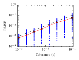
(a) Case q = 1.

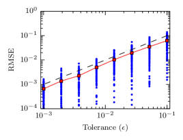
(b) Case q = 2.

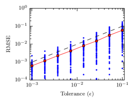
(c) Case q = 3.

(d) Legend.

Figure 2: RMSE (square markers and line) plotted vs. tolerance for the experiment described in Section 8.1. The dashed line is the tolerance $\epsilon$ and the dots are the individual errors for the $100$ runs at each tolerance.

In order to verify Theorem 10, we estimated the expected cost for each tolerance $\epsilon$ and value of $q$ by computing the mean of the total cost over the $100$ runs. The cost for each realization was computed using the cost model in equation (10). The cost for realizations differs not only between levels $\ell$, but also within a level $\ell$ owing to the selective refinement algorithm. For each run $i$, the costs of all realizations were summed to obtain the total cost for that run. We computed a mean of the total costs for the $100$ runs. A plot of the result can be found in Figure 3. As the tolerance $\epsilon$ decreases the expected cost approaches the rates given in Theorem 10. The reference costs are multiplied by constants to align well with the estimated expected costs.

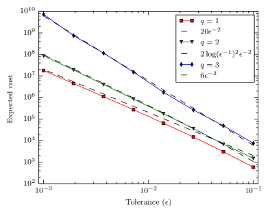
Figure 3: Computed mean total cost (diamond, triangle, square markers and lines) plotted with theoretical reference cost (dashed lines) for the experiment described in Section 8.1. The reference costs for the three values of $q$ are: $20\epsilon^{-2}$ for $q=1$; $2\log(\epsilon^{-1})^{2}\epsilon^{-2}$ for $q=2$; and $6\epsilon^{-3}$ for $q=3$.

8.2 Single-phase flow in media with lognormal permeability

We consider Darcy’s law on a unit square $[0,1]^{2}$ on which we have impearmeable upper and lower boundaries, high pressure on the left boundary ($\Gamma_{1}$) and low pressure on the right boundary ($\Gamma_{2}$). We define the spaces $H^{1}_{f}(\mathscr{D})=\{v\in H^{1}(\mathscr{D}):v|_{\Gamma_{1}}=f\text{ and }v|_{\Gamma_{2}}=0\}$, and let $n$ denote the unit normal of $\mathscr{D}$.

The weak form of the partial differential equation reads: find $u\in H^{1}_{1}(\mathscr{D})$ such that

$$(a(\omega,\cdot)\nabla u,\nabla v)=0\quad\text{ in }\mathscr{D},$$ (21)

for all $v\in H_{0}^{1}(\mathscr{D})$, and $a$ is a stationary log-normal distributed random field

$$a(\omega,\cdot)=\exp(\kappa(\omega,\cdot)),$$ (22)

over $\mathscr{D}$, where $\kappa(\cdot,x)$ has zero mean and is normal distributed with exponential covariance, i.e., for all $x_{1},x_{2}\in\mathscr{D}$ we have that

$$\mathbb{V}\mathopen{}\mathclose{{}\left[\kappa(\cdot,x_{1})\kappa(\cdot,x_{2})}\right]=\sigma^{2}\exp\mathopen{}\mathclose{{}\left(\frac{-\|x_{1}-x_{2}\|_{2}}{\rho}}\right).$$ (23)

We choose $\sigma=1$ and $\rho=0.1$ in the numerical experiment.

We are interested in the boundary flux on the right boundary, i.e., the functional $X(\omega)=\int_{\Gamma_{2}}n\cdot a(\omega)\nabla u\,\mathrm{d}x=(a(\omega,\cdot)\nabla u,\nabla g)$, for any $g\in H^{1}(\mathscr{D})$, $g|_{\Gamma_{1}}=0$ and $g|_{\Gamma_{2}}=1$. The last equality comes by a generalized Green’s identity, see [10, Chp. 1, Corollary 2.1].

To generate realizations of $a(\omega,\cdot)$, the circulant embedding method introduced in [5] is employed. The mesh resolution for the input data of the realizations generated on level $\ell$ in the MLMC-SR algorithm is chosen such that the finest mesh needed on level $\ell$ is not finer than the chosen mesh. For a fixed realization on level $\ell$ we don’t know how fine data we need, because of the selective refinement procedure. This means that the complexity obtained for the MLMC-SR algorithm do not apply for the generation of data. The circulant embedding method has log-linear complexity. A remedy for the complexity of generating realizations is to use a truncated Karhunen-Loève expansion that can easily be refined. However, numerical experiments show that we are in a regime where the time spent on generating realizations using circulant embedding is negligible compared to the time spent in the linear solvers.

The PDE is discretized using a FEM-discretization with linear Lagrange elements. We have a family of structured nested meshes $\mathcal{T}_{h_{m}}$, where a mesh $h_{m}$ is the maximum element diameter of the given mesh. The data $a(\omega,\cdot)$ is defined in the grid points of the meshes. Using the circulant embedding we get an exact representation of the stochastic field in the grid points of the given mesh. This can be interpreted as not making any approximation of the stochastic field but instead making a quadrature error when computing the bilinear form.

The functional for a discretization on mesh $m$ is defined as $X_{h_{m}}(\omega)=(a(\omega,\cdot)\nabla u_{h_{m}},\nabla g)$. The convergence rates in energy norm for log-normal data is $h^{1/2-\delta}$ for any $\delta>0$ [2]. Using postprocessing, it can be shown that the error in the functional converges twice as fast [9], i.e, $|X_{h_{m}}-X_{h_{m}}(\omega)|\leq Ch^{s-2\delta}$ for $s=1$. We use a multigrid solver that has linear $\alpha=1$ (up to $\log$-factors) complexity. The work for one sample can then be computed as $\gamma^{-q\ell}$ where $\gamma^{\ell}$ is the numerical bias tolerance for the sample and $q\approx 2\alpha/s=2$, which was also verified numerically. The error is estimated using the dual solution computed on a finer mesh. Since it can be quite expensive to solve a dual problem for each realization of the data, the error in the functional can also be computed by estimating the constant $C$ and $s$ either numerically or theoretically.

We choose $\gamma=0.5$, $N=10$, and $k=1$ in the the MLMC-SR algorithm, see Section 7 for more information on the choices of parameters. The problem reads: find the probability $p$ for $X\leq y=1.5$ to the given RMSE $\epsilon$. We compute $p$ for $\epsilon=10^{-1}$, $10^{-1.5}$, and $10^{-2}$. All parameters used in the simulation are presented in Table 3.

Parameter	Value
$y$	$1.5$
$q$	$2$
$\gamma$	$0.5$
$N$	$10$
$k$	$1$
$\epsilon$	$10^{-1},10^{-1.5},10^{-2}$
$\rho$	$0.1$
$\sigma$	$1$

Table 3: Parameters used for the single-phase flow experiment. The parameters $y,q,\gamma,N,k,\epsilon$ are used in the MLMC-SR algorithm and $\rho$, $\sigma$ to define the log-normal field.

To verify the accuracy of the estimator we compute $100$ simulations of the MLMC-SR estimator for each RMSE $\epsilon$ and present the sample standard deviation (square root of the sample variance) of the MLMC-SR estimators in Table 4.

$\epsilon$	Mean $p$	Sample std	Target std ($\epsilon/\sqrt{2}$)
$10^{-1}$	$0.8834$	$6.472\cdot 10^{-2}$	$7.071\cdot 10^{-2}$
$10^{-1.5}$	$0.8890$	$1.873\cdot 10^{-2}$	$2.236\cdot 10^{-2}$
$10^{-2}$	$0.8933$	$5.557\cdot 10^{-2}$	$7.071\cdot 10^{-3}$

Table 4: The mean failure probability $p$ and sample standard deviation (std) is computed using 100 MLMC-SR estimators and compared to the target std which is the statistical part of the RMSE error $\epsilon$.

We see that in all the three cases the sample standard deviation is smaller than the statistical contribution $\epsilon/\sqrt{2}$ of the RMSE $\epsilon$. Since the exact flux is unknown, the numerical contribution in the estimator has to be approximated to be less than $\epsilon/\sqrt{2}$ as well, which is done in the termination criterion of the MLMC-SR algorithm so it is not presented here. The mean number of samples computed to the different tolerances on each level of the MLMC-SR algorithm is computed from 100 simulations of the MLMC-SR estimator for $\epsilon=10^{-2}$ and are shown in Table 5.

$\ell$	$0$	$1$	$2$	$3$	$4$
Mean $N_{\ell}$	$16526.81$	$9045.41$	$4524.83$	$1471.63$	$738.63$
$j=0$	$16526.81$	$4520.99$	$2265.23$	$734.21$	$366.9$
$j=1$		$4524.42$	$1486.62$	$484.11$	$244.69$
$j=2$			$772.98$	$232.33$	$116.77$
$j=3$				$20.98$	$9.76$
$j=4$					$0.51$

Table 5: The distribution of realizations solved to different tolerance levels $j$ for the case $\epsilon=10^{-2}$. The table is based on the mean of $100$ runs.

The table shows that the selective refinement algorithm only refines a fraction of all problems to the highest accuracy level $j=\ell$. Using a MLMC method (without selective refinement) $N_{\ell}$ problem would be solved to the highest accuracy level. Using the cost model $\gamma^{-q\ell}$ for $\epsilon=10^{-2}$ we gain a factor $\sim 6$ in computational cost for this particular problem using MLMC-SR compared to MLMC. From Theorem 10 the computational cost for MLMC-SR and MLMC increase as $\epsilon^{-2}\log(\epsilon^{-1})^{2}$ and $\epsilon^{-3}$, respectively.

Appendix A Derivation of optimal level sample size

To determine the optimal sample level size $N_{\ell}$ in equation (7), we minimize the total cost keeping the variance of the MLMC estimator equal to $\epsilon^{2}/2$, i.e.,

min $$\sum_{\ell=0}^{L}N_{\ell}c_{\ell}$$ (24)

subject to $$\sum_{\ell=0}^{L}N_{\ell}^{-1}\mathbb{V}\mathopen{}\mathclose{{}\left[Y_{\ell}}\right]=\epsilon^{2}/2,$$

where $Y_{\ell}=Q_{\ell}-Q_{\ell-1}$. We reformulate the problem using a Lagrangian multiplier $\mu$ for the constraint. Define the objective function

$$g(N_{\ell},\mu)=\sum_{\ell=0}^{L}N_{\ell}c_{\ell}+\mu\mathopen{}\mathclose{{}\left(\sum_{\ell=0}^{L}N_{\ell}^{-1}\mathbb{V}\mathopen{}\mathclose{{}\left[Y_{\ell}}\right]-\epsilon^{2}/2}\right).$$ (25)

The solution is a stationary point $(N_{\ell},\mu)$ such that $\nabla_{N_{\ell},\mu}g(N_{\ell},\mu)=0$. Denoting by $\hat{N}_{\ell}$ and $\hat{\mu}$ the components of the gradient, we obtain

$$\nabla_{N_{\ell},\mu}g(N_{\ell},\mu)=\mathopen{}\mathclose{{}\left(c_{\ell}-\mu N_{\ell}^{-2}\mathbb{V}\mathopen{}\mathclose{{}\left[Y_{\ell}}\right]}\right)\hat{N}_{\ell}+\mathopen{}\mathclose{{}\left(\sum_{\ell=0}^{L}N_{\ell}^{-1}\mathbb{V}\mathopen{}\mathclose{{}\left[Y_{\ell}}\right]-\epsilon^{2}/2}\right)\hat{\mu}.$$ (26)

Choosing $N_{\ell}=\sqrt{\mu\mathbb{V}\mathopen{}\mathclose{{}\left[Y_{\ell}}\right]/c_{\ell}}$ makes the $\hat{N}_{\ell}$ components zero. The $\hat{\mu}$ component is zero when $\sum_{\ell=0}^{L}N_{\ell}^{-1}\mathbb{V}\mathopen{}\mathclose{{}\left[Y_{\ell}}\right]=\epsilon^{2}/2$. Plugging in $N_{\ell}$ yields $2\epsilon^{-2}\sum_{\ell=0}^{L}\sqrt{\mathbb{V}\mathopen{}\mathclose{{}\left[Y_{\ell}}\right]c_{\ell}}=\sqrt{\mu}$ and hence the optimal sample size is

$$N_{\ell}=2\epsilon^{-2}\sqrt{\mathbb{V}\mathopen{}\mathclose{{}\left[Y_{\ell}}\right]/c_{\ell}}\sum_{k=0}^{L}\sqrt{\mathbb{V}\mathopen{}\mathclose{{}\left[Y_{k}}\right]c_{k}}.$$ (27)

References

- [1] S.-K. Au and J. L. Beck. Estimation of small failure probabilities in high dimensions by subset simulation. Probabilistic Engineering Mechanics, 16(4):263–277, 2001.
- [2] J. Charrier, R. Scheichl, and A. L. Teckentrup. Finite element error analysis of elliptic PDEs with random coefficients and its application to multilevel Monte Carlo methods. SIAM J. Numer. Anal., 51(1):322–352, 2013.
- [3] K. A. Cliffe, M. B. Giles, R. Scheichl, and A. L. Teckentrup. Multilevel Monte Carlo methods and applications to elliptic PDEs with random coefficients. Comput. Vis. Sci., 14(1):3–15, 2011.
- [4] N. Collier, A.-L. Haji-Ali, F. Nobile, E. von Schwerin, and R. Tempone. A Continuation Multilevel Monte Carlo algorithm. ArXiv e-prints:1402.2463, 2014.
- [5] C. Dietrich and G. Newsam. Fast and exact simulation of stationary gaussian processes through circulant embedding of the covariance matrix. SIAM J. Sci. Comput., 18(4):1088–1107, 1997.
- [6] D. Elfverson, D. Estep, F. Hellman, and A Mlqvist. Quantile bounds for numerical models with data uncertainty. Preprint, 2014.
- [7] D. Estep, A. Mlqvist, and S. Tavener. Nonparametric density estimation for randomly perturbed elliptic problems. I. Computational methods, a posteriori analysis, and adaptive error control. SIAM J. Sci. Comput., 31(4):2935–2959, 2009.
- [8] M. B. Giles. Multilevel Monte Carlo path simulation. Oper. Res., 56(3):607–617, 2008.
- [9] M. B. Giles and E. Süli. Adjoint methods for PDEs: a posteriori error analysis and postprocessing by duality. Acta Numer., 11:145–236, 2002.
- [10] V. Girault and P.-A. Raviart. Finite element methods for Navier-Stokes equations, volume 5 of Springer Series in Computational Mathematics. Springer-Verlag, Berlin, 1986. Theory and algorithms.
- [11] P. Glasserman, P. Heidelberger, P. Shahabuddin, and T. Zajic. Splitting for rare event simulation: analysis of simple cases. In Proceedings of the 1996 Winter Simulation Conference, pages 302–308, 1996.
- [12] P. Glynn. Importance sampling for monte carlo estimation of quantiles. In Mathematical Methods in Stochastic Simulation and Experimental Design: Proc. 2nd St. Petersburg Workshop on Simulation (Publishing House of Saint Petersburg University), pages 180–185, 1996.
- [13] A.-L. Haji Ali, F. Nobile, E. von Schwerin, and R. Tempone. Optimization of mesh hierarchies in Multilevel Monte Carlo samplers. ArXiv e-prints:1403.2480, 2014.
- [14] E. Jones, T. Oliphant, P. Peterson, et al. SciPy: Open source scientific tools for Python, 2001–. [Online; accessed 2014-08-22].
- [15] A. Kebaier. Statistical romberg extrapolation: a new variance reduction method and applications to options pricing. Annals of Applied Probability, 14(4):2681–2705, 2005.
- [16] A. Logg, K.-A. Mardal, and G. Wells. Automated Solution of Differential Equations by the Finite Element Method, volume 84 of Lecture Notes in Computational Science and Engineering. Springer, Berlin Heidelberg, 2012.
- [17] A. L. Teckentrup, R. Scheichl, M. B. Giles, and E. Ullmann. Further analysis of multilevel Monte Carlo methods for elliptic PDEs with random coefficients. Numer. Math., 125(3):569–600, 2013.