Numerical simulations of nonlinear modes in mica: past, present and future

Abstract.

We review research on the role of nonlinear coherent phenomena (e.g breathers and kinks) in the formation linear decorations in mica crystal. The work is based on a new model for the motion of the mica hexagonal K layer, which allows displacement of the atoms from the unit cell. With a simple piece-wise polynomial inter-particle potential, we verify the existence of localized long-lived breathers in an idealized lattice at 0^∘K. Moreover, our model allows us to observe long-lived localized kinks. We study the interactions of such localized modes along a lattice direction, and in addition demonstrate fully two dimensional scattering of such pulses for the first time. For large interatomic forces we observe a spreading horseshoe-shaped wave, a type of shock wave but with a breather profile.

1. Introduction

The role of nonlinear localized coherent phenomena for the formation of anomalous structures in crystalline materials remains unclear, despite a number of efforts over the last two decades. In this article, we begin with a short survey of the state of the art in research on this topic. This serves to introduce a number of relevant issues in relation to atomistic models, including the work of Marín et al. on breathers [16] in the K layer in mica.

From a heavily simplified perspective, there are three types of localized excitations in dispersive nonlinear systems. These are (in 1D) solitons, kinks, and breathers, as illustrated in Fig. 1.

• Soliton. Strongly localized package (lump) of energy, can move large distances with no distortion, very stable even under collisions or perturbations.

• Kink. Similar to a soliton, but with different boundary conditions as $x\rightarrow\pm\infty$. May be even more stable due to topological conservation laws.

• Breather. A more complicated form of nonlinear wave. It looks like a soliton modulated by an internal carrier wave. Not common in continuous systems but more frequently seen in discrete systems.

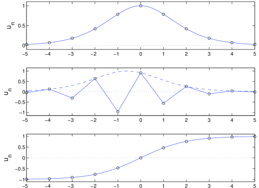
Figure 1. Solitons, breathers and kinks, in 1D discrete lattices.

Note that breathers are also known as Intrinsic Localized Modes (ILMs). M. Russell’s quodon discussed in this article is now believed to be a breather.

Breathers in discrete systems were first studied by Ovchinnikov [19], but this pioneering paper was overlooked for many years. Ovchinnikov also considered the mobility of such objects.

Independently in the early ’80s, breathers were studied in the Discrete Nonlinear Schrödinger (DNLS) equation.

$${\rm i}\frac{\textrm{d}A_{j}}{\textrm{d}t}+(A_{j-1}-2A_{j}+A_{j+1})+\gamma|A_{j}|^{2}A_{j}=0\;,$$

where $A_{j}(t)$ is the complex oscillator amplitude at the $j$th lattice site. An early application of the DNLS equation was as a simple model for so-called Davydov solitons on a protein molecule. Arguably the first paper on the single breather in the system was due to Scott and MacNeil [23] (although such states were still called solitons in the early papers).

Figure 2. Breather, DNLS equation.

Fig. 2 shows a stationary breather on the DNLS lattice. The time dependence in the DNLS model for stationary solutions is extremely simple: $A_{n}(t)=\phi_{n}\exp(i\omega t)$. The amplitude goes to zero exponentially as $|n|\rightarrow\infty$. Eilbeck, Lomdahl and Scott took the first tentative step towards a 2D theory of breathers in the DNLS model by considering two coupled chains in a study of a crystal called Acetanilide (ACN) which modelled protein structure [7]. This work found examples of staggered breathers (i.e. breather energies spread over two or more sites) and the use of path-following from what is now called the anti-continuum limit. They also considered more complex non-chain geometries, finding many exact solutions on small graphs [8]. In the course of work in this area, a relatively long-lived example of a moving breathers in a 1D discrete systems was found [6], see Fig. 3.

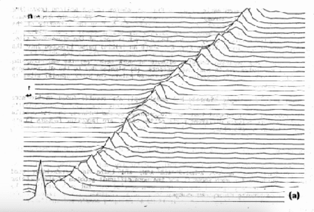
Figure 3. Moving breather in a simple model system (DNLS). Here energy is plotted rather than complex amplitude.

Many workers found other examples of discrete breathers in various systems (see [10, 11] for reviews). In 1994, MacKay and Aubry found a general mathematical proof for the existence of stationary breathers in a quite general class of systems [14]. For mobile breathers in the DNLS equation, Feddersen found a very accurate numerical description of travelling wave solutions in 1991 [9, 5].

The study of kinks in continuum and discrete models is a large subject in its own right. A good early paper by Peyrard and Kruskal [20], on kinks in a highly discrete sine-Gordon model, is a nice introduction. Some results on the numerical studies of solitons in discrete systems will be found in [5].

1.1. Solitons, kinks and breathers in 2D

It is not difficult to generalise soliton or kink equations to give models which have plane wave solutions in 2D, see Fig. 4.

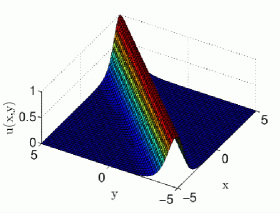
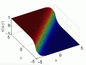
Figure 4. Soliton on the left, kink on the right.

However there is a problem - the wave front has a finite energy density so the infinite wave front has infinite energy. What we need is a localized pulse with finite energy.

Schematically we can envisage pulses such as that shown in Fig. 5.

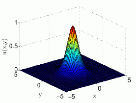
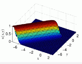
Figure 5. Localized soliton (left), candidate for a kink on the right, travelling from left to right.

The soliton looks reasonable, but for topological reasons the kink has an infinite “side wall” dislocation which may lead to infinite energy. The tail can be truncated–but this brings us back to a soliton-type wave. The challenge then is to develop a suitable model for a kink or soliton solution in a 2D system, or failing that to find breather solutions.

1.1.1. Derrick’s theorem

In a simple single component homogeneous scalar continuum field theory, we have a non-existence proof for stationary solitons due to Derrick (see [15]). The simple idea is to start by supposing that, for example, our $n$-dimensional Hamiltonian is

$$E(\phi) = \int\left(W(\phi)\nabla(\phi)\cdot\nabla(\phi)+U(\phi)\right)\,\textrm{d}^{n}x$$

$$\equiv E_{2}+E_{0}\;.$$

Consider scaling the spatial variable $\vec{x}\rightarrow\mu\vec{x}$. It is easy to show that

$$E(\phi(\mu\vec{x}))=\mu^{2-n}E_{2}+\mu^{-n}E_{0}\;.$$

If the soliton solution $\phi(\vec{x})$ is a stable minima, then $\textrm{d}{E}/\textrm{d}\mu=0$. The solution for $n=1$ is $\mu=\sqrt{E_{0}/E_{2}}$, but there is no solution for $n=2,3$.

Note that the theorem does not apply when we have a discrete system which does not have a continuum limit - here breathers/ILMs/quodons may play a part. The theorem (and the arguments given following the figures above) give an indication that problems may arise if we try to generalise in a naive way from 1D to higher dimensions.

1.2. The work of Marín et al. on breathers in the K layer of mica

Russell’s work on mica led to Collins preparing a potential energy plot on the Potassium layer - the energy of moving one $\mathbf{K}$ atom with all the others being fixed [21], see Fig. 6.

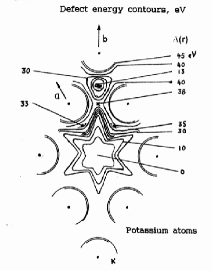
Figure 6. Energy levels in the K layer in Mica.

In 1998, Marín et al. [16] used the quantitative features of this plot to make a careful numerical study of a simple 2D model of the K layer in mica. His program hexlatt simulates the motion of a classical 2D hexagonal lattice, with displacements in the plane. It includes both a nonlinear nearest-neighbour coupling ($W$) between the $\mathbf{K}$ and some type of nonlinear “on-site” potential ($V$) [16]. The Hamiltonian is

(1.1) $$H=\sum_{i,j}\frac{1}{2}\|\dot{\vec{u}}_{i,j}\|^{2}+V(\vec{u}_{i,j})+\frac{1}{2}\lambda\sum_{i^{\prime},j^{\prime}}W(\vec{u}_{i,j},\vec{u}_{i^{\prime},j^{\prime}})\;,$$

where $\vec{u}_{i,j}$ is the $(i,j)$th atom’s displacement from its equilibrium state, and $\dot{\vec{u}}_{i,j}$ is the displacement’s time derivative. For the on-site potential (mimicking the effect of the $\mathbf{O}$ atoms above and below the $\mathbf{K}$ plane, assumed fixed) he used 6 atoms interacting in a Morse potential:

(1.2) $$V_{\mbox{Morse}}(s)=\frac{1}{2}(1-\exp(-s))^{2}\;,$$

where $s$ is the distance between potassium and fixed oxygen atoms. For interatomic potential ($\mathbf{K}$-$\mathbf{K}$) he used a scaled classical 6-12 Lennard-Jones

$$W_{\mbox{LJ}}(r)=1+\left(\frac{\sigma}{r}\right)^{12}-2\left(\frac{\sigma}{r}\right)^{6}\;,$$

where $r$ is the distance between neighbouring potassium atoms and $\sigma$ is a lattice constant. The best results were found when both the on-site and interatomic potentials have similar strengths. Fig. 7 shows one typical simulation on a 16x16 lattice.

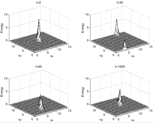
Figure 7. Breather motion in model hexagonal lattice.

Note that we plot local energy density at various times on the lattice. At $t=0$ we give three atoms in the centre an asymmetric kick, to mimic the radioactive decay of a K atom in the mica. At $t=30$ the breather resulting from this kick has moved to the edge of the small lattice and is beginning to reappear on the opposite side due to the imposed periodic boundary conditions. At $t=60$ it has continued in the same direction and has almost reached the starting point. The final frame is at a much later time, $t=1000$, and shows the breather after it has traversed the lattice about ten times.

Marín’s study showed stable breathers propagating up to around $\leq$ $10^{4}$ lattice constants before breaking up. This is encouraging, but to demonstrate tracks in mica of centimetres, we need an extra factor of $10^{5}$ in the lifetime. Marín’s 2D calculation also included a brief study of inline breather-breather collisions [17]. Most simulations were performed on a 16x16 lattice due to CPU speeds at the time, but a few were done using 32x32 lattices. The K atoms were constrained to stay within the unit cell–with no hopping to other sites (hence no kinks). All simulations were carried out at zero temperature. Similar results were also observed for cubic lattices [18].

A key feature in the model is that the forces have the so-called quasi-one-dimensional property–that is, if an atom is moved along one of the crystallographic directions, the restoring forces is exactly in the same line, but with a negative sign. Technically this is a $C_{2}$ symmetry. Note that we also use “quasi-one-dimensional” in a different sense, to describe the fact that a localized breather or kink is observed travelling along a crystallographic direction with very little disturbance in a transverse direction. The two concepts are conjectured to be closely related, although no formal proof of this exists.

  Historical Anecdote.   The second author’s involvement in this problem began in 1995, when he was contacted for the first time by Mike Russell. Mike was interested in attending the soliton and nonlinear waves meeting, photo shown in Fig. 8, that JCE was organising in Edinburgh that summer. He was keen to discuss nonlinear effects in mica crystal.

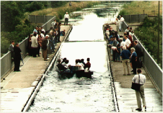
Figure 8. Recreation of the soliton on the Union canal in 1995.

Mike was studying the tracks in mica as seen in Fig. 9 and believed that these could provide evidence for some sort of nonlinear wave like a soliton in a 2D crystal - no linear theory seemed to fit the data.

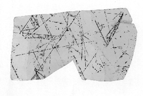
Figure 9. Tracks in mica, several cm long.

JCE had long been interested in nonlinear waves, initially in continuous systems, but more recently in discrete systems. JCE, at that time, was especially interested in breathers in lattices. Subsequent collaboration of the two led to a series of papers aimed at understanding the theoretical underpinnings of the mica tracks (among other phenomena).

Although the consequent papers of Marín, Eilbeck and Russell received some attention, the calculations have never been replicated. The Altea meeting in Spain in 2013 provided an excellent opportunity to revisit and extend these calculations. What follows is a more extensive examination of results based on the simple model we presented there.

 

2. Preliminary results from numerical experiments

In the main part of this section, we describe a new 2D mathematical model used for the present study of long-lived propagating breather and kink solutions in mica at 0^∘K. With this model we allow atoms in the lattice to be displaced out of the unit cells compared to the nearest neighbour interactions considered in Marín’s model from Sect. 1.2. Thus we can now allow the possibility of kink solutions in our 2D lattice model. In addition, in the choice of potentials we take a more academic point of view and explore alternative approaches besides Lennard-Jones. Current research raises new and not yet fully understood questions, and motivates further, more intensive study.

In the present work we are concerned with the Hamiltonian dynamics of $N$ potassium atoms $\mathbf{K}$ in a 2D $\mathbf{K}$-$\mathbf{K}$ sheet of mica crystal lattice. Equivalently to (1.1) the Hamiltonian of the system is

(2.3) $$H=K+V+U=\sum_{n=1}^{N}\left(\frac{1}{2}\|\vec{u}_{n}\|^{2}+\sum_{n^{\prime}=1,\,n^{\prime}\neq{n}}^{N}V(\vec{r}_{n},\vec{r}_{n^{\prime}})+U(\vec{r}_{n})\right)\;,$$

where $\vec{r}_{n}\in\mathrm{R}^{2}$ is the 2D position vector of $n^{th}$ $\mathbf{K}$ atom in $(x,y)$ coordinates, $\vec{u}_{n}=\dot{\vec{r}}_{n}$ is momentum, $K$ is kinetic energy, $V$ is the interaction potential energy and $U$ is the on-site potential energy. All masses of atoms are normalized to one. The system of equations is

(2.4) $$\dot{\vec{r}}_{n} = \vec{u}_{n}\;,$$

(2.5) $$\dot{\vec{u}}_{n} = -\partial_{\vec{r}_{n}}\left(\sum_{n^{\prime}=1,\,n^{\prime}\neq{n}}^{N}V(\vec{r}_{n},\vec{r}_{n^{\prime}})+U(\vec{r}_{n})\right)\;,$$

for all $n=1,\dots,N$.

2.1. On-site potential

In contrast to the on-site potential (1.2) considered by Marín et al. [16], but with the same assumptions of the fixed upper and lower layers of oxygen atoms, we consider a smooth periodic function with hexagonal symmetry [24], i.e. a function resembling an egg-box carton

(2.6) $$U(x,y) = \frac{2}{3}U_{0}\Bigg{(}1-\frac{1}{3}\Bigg{(}\cos{\Bigg{(}\frac{4\pi{y}}{\sqrt{3}\sigma}\Bigg{)}}$$

$$+\cos{\Bigg{(}\frac{2\pi(\sqrt{3}x-y)}{\sqrt{3}\sigma}\Bigg{)}}+\cos{\Bigg{(}\frac{2\pi(\sqrt{3}x+y)}{\sqrt{3}\sigma}\Bigg{)}}\Bigg{)}\Bigg{)}\;,$$

where $x=(\vec{r}_{n})_{1}$, $y=(\vec{r}_{n})_{2}$, $\sigma$ is the lattice constant and $U_{0}>0$ is the maximal value of the on-site potential, see Fig. 1010A. This model has the same quantitative features as Fig. 6.

Note that a simple product of cosine functions would not provide the required hexagonal symmetry. Also, in a 1D approximation, i.e. $y=\mbox{const.}$, the on-site potential (2.6) reduces to the cosine function which is an on-site potential of the discrete sine-Gordon equation and the periodic potential of a 1D model considered in [4]. The model in [4] can be thought as a 1D approximation of the 2D model (2.3) in any of three crystallographic lattice directions which can be prescribed by the direction cosines, that is, with vectors: $(1,0)^{T}$ and $(1/2,\pm\sqrt{3}/2)^{T}$. Without periodic boundary conditions, a smooth cut-off of potential (2.6) can be imposed.

]6cm

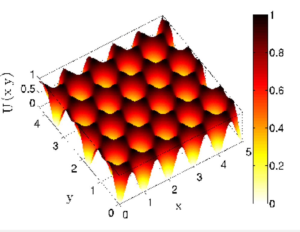
10A Egg-box carton on-site potential with $\sigma=1$ and $U_{0}=1$.

]6cm

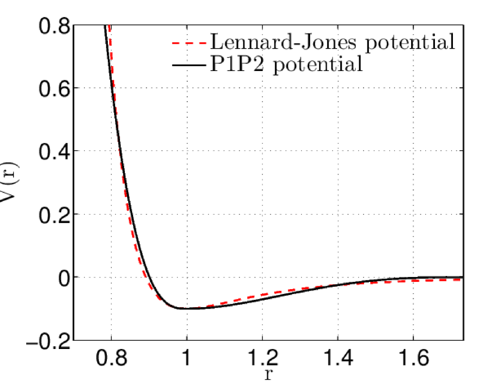
10B Comparison between the Lennard-Jones potential and the polynomial potential ($P_{1}P_{2}$) with $M=25$, $\epsilon=0.1$, $\sigma=1$ and $r_{cut}=\sqrt{3}\sigma$.

2.2. Interaction potential $\mathbf{(P_{1}P_{2})}$

There are very well known and much used empirical interaction potentials from the molecular dynamics community such as Lennard-Jones 12-6, Morse and Buckingham potentials, among others. Essentially all of these interaction potentials model repulsive and attractive forces of particles. The detailed structure of these potential energy functions may strongly influence the behaviour observed in simulations, particularly dynamical properties.

All potentials mentioned above are built from completely monotone functions with a possible singularity at vanishing interparticle distance. For example, the Lennard-Jones 12-6 potential has been extensively used in molecular dynamics models, on account of its good representation of van der Waals attraction forces and its efficient implementation in numerical codes. In this article, we use a simple family of interaction potentials, defined by piecewise polynomials, which allow for easy adjustment of modelling features such as well depth and which do not have a singularity at the origin. Importantly we have found that these simplified potentials lead to interesting properties of the numerical solutions for our lattice model compared to those obtained using more conventional interaction potentials (in particular, we observe kinks in certain simulations, see below.) We refer the interested reader to [2] where the authors have performed a numerical study of propagating localized modes in a 2D hexagonal lattice, by considering conventional Lennard-Jones potential for the interparticle interactions and the same on-site potential (2.6).

The numerical results observed in this article suggest the need for deeper analytical investigations, particularly where these may lead to the design of completely new materials [12]. In addition, the use of piecewise polynomial potentials may provide additional freedom to better match the material properties in consideration, while excluding singularities and directly incorporating smooth cut-offs; such potentials can be constructed to different orders of regularity.

In this paper, for the interaction potential $V$, we consider a distance dependant potential of two joint $4^{th}$ order polynomials $P_{1}(r)$ and $P_{2}(r)$, that is

$$V(r)=\left\{\begin{array}[]{l l}P_{1}(r)\;,&\quad 0\leq r\leq\sigma\;,\\ P_{2}(r)\;,&\quad\sigma<r\leq r_{cut}\;,\\ 0\;,&\quad\mbox{otherwise}\;,\end{array}\right.$$

where $r=\|\vec{r}_{n}-\vec{r}_{n^{\prime}}\|$ for all $n$ and $n^{\prime}$, $n\neq{n^{\prime}}$. The parameter $\sigma$ is the lattice constant and $r_{cut}$ is the cut-off radius of the potential. The coefficients of the polynomials $P_{1}(r)$ and $P_{2}(r)$ are found from the following constraints:

$$P_{1}(0)=M\;,\quad\partial_{r}P_{1}(0)=0\;,\quad M>0\;,$$

$$P_{1}(\sigma)=P_{2}(\sigma)=-\epsilon\;,\quad\epsilon>0\;,$$

$$\partial_{r}{P}_{1}(\sigma)=\partial_{r}{P}_{2}(\sigma)=0\;,$$

$$\partial_{rr}{P}_{1}(\sigma)=\partial_{rr}{P}_{2}(\sigma)\;,$$

$$P_{2}(r_{cut})=0\;,\quad\partial_{r}{P}_{2}(r_{cut})=0\;,\quad\partial_{rr}{P}_{2}(r_{cut})=0\;,$$

such that $V(0)=M$, $V(\sigma)=-\epsilon$, $V(r_{cut})=0$, $\partial_{r}V(0)=0$, $\partial_{r}V(\sigma)=0$, $\partial_{r}V(r_{cut})=0$ and $\partial_{rr}V(r_{cut})=0$.

For small atomic displacements from the mechanical equilibrium state, which we will consider as our initial conditions, the particular choice of the cut-off radius $r_{cut}=\sqrt{(}3)\sigma$ leads to the closest representation of the nearest neighbour interaction model, i.e. Hamiltonian dynamics of atoms with only nearest neighbour interactions, such as the model by Marín et al. [16]. Importantly, there is no formal restrictions to consider larger values of the cut-off radius $r_{cut}$.

For our computations we choose $\sigma=1$, $M=25$ and $\epsilon=0.1$ to approximately match the scaled Lennard-Jones potential

$$V_{LJ}(r)=\epsilon\left(\left(\frac{\sigma}{r}\right)^{12}-2\left(\frac{\sigma}{r}\right)^{6}\right)$$

with $\sigma=1$ and $\epsilon=0.1$, where $\sigma$ is the same lattice constant and $\epsilon$ is the potential well depth value, see Fig. 1010B. Additional motivation for the particular choice of parameter values will be given in Sec. 2.4.

2.3. Time integration method

In simulations of Hamiltonian systems, e.g. (2.4)–(2.5), it is essential to use a symplectic time integration procedure. In our simulations, we employed the Verlet method, a second order, explicit symplectic scheme [1, 13]. The method is known for its good energy conservation properties in long time simulations where energy stays bounded in time and is conserved up to second order with respect to a time step. For a Hamiltonian of the form $H=\frac{1}{2}\|\vec{p}\|^{2}+V(\vec{q})$, the Verlet timestep approximates Newtonian dynamics by the steps:

$$\vec{q}^{n+1/2} = \vec{q}^{n}+\frac{1}{2}\tau\vec{p}^{n}\;,$$

$$\vec{p}^{n+1} = \vec{p}^{n}-\tau\nabla_{\vec{q}}V(\vec{q}^{n+1/2})\;,$$

$$\vec{q}^{n+1} = \vec{q}^{n+1/2}+\frac{1}{2}\tau\vec{p}^{n+1}\;,$$

where $\tau$ is the time step, $\vec{q}^{n}\approx\vec{q}(t^{n})$ and $\vec{p}^{n}\approx\vec{p}(t^{n})$ at time level $t^{n}=n\tau$ where $n=0,1,\dots$. As mentioned above, the method preserves the symplectic property of Hamiltonian dynamics, i.e. $\textrm{d}\vec{q}^{n+1}\wedge\textrm{d}\vec{p}^{n+1}=\textrm{d}\vec{q}^{n}\wedge\textrm{d}\vec{p}^{n}$, where $\wedge$ is a wedge product of two differential 1-forms in vector representation. Thus the model is also volume preserving in phase space. A valuable feature of symplectic integrators is that they may, under certain circumstances, be interpreted as being essentially equivalent to the exact propagation of a modified Hamiltonian ($\tilde{H}_{\tau}=H+O(\tau^{k})$) (for a $k^{th}$ order scheme) meaning that we may reinterpret the trajectories generated by our numerical method as dynamical paths for a perturbed system. Interested readers in numerical methods for Hamiltonian dynamics are referred to [13].

2.4. Parameter values

To proceed with the numerical study of propagating localized modes of system (2.4)–(2.5) we must select system parameter values. Without loss of generality, we set the lattice constant $\sigma$ equal to one. Once the interaction potential parameter values are fixed, we are left with one parameter value to consider, that is, the strength of the on-site potential parameter $U_{0}$. Thus with the parameter $U_{0}$ we can control the relative strengths of forces in the system. With very small values of $U_{0}$, the system will be dominated by the forces of the interaction potential, and vice versa.

As was noted by Marín et al. [16], the best conditions to observe propagating discrete breathers seemed to be when both potentials are of roughly equal strength. We find that for given interaction potential parameter values $r_{cut}=\sqrt{3}\sigma$, $\sigma=1$, $M=25$ and $\epsilon=0.1$, and with value $U_{0}=2$, both potentials agree well for the small displacements of the potassium $\mathbf{K}$ atom from its mechanical equilibrium state while the neighbouring $\mathbf{K}$ atoms have been fixed in their positions. For the comparison of potentials we consider an atom with the six fixed neighbouring atoms in their equilibrium states.

Results of unrelaxed potential computations are shown in Fig. 11 for the parameter values given above. In both plots we normalize the interaction potential values such that $V\geq{0}$. In the left plot of Fig. 11, we compute unrelaxed potentials as seen by an $\mathbf{K}$ atom moving in the $(1,0)^{T}$ crystallographic direction in a 2D $\mathbf{K}$-$\mathbf{K}$ sheet of mica crystal lattice, while in the right plot of Fig. 11 we plot the total potential energy contour lines as seen by the $\mathbf{K}$ atom at origin. The colour axis agrees with the location of the $\mathbf{K}$ atom in space. When the atom is at the origin, the total potential energy is equal to zero. However when the atom approaches any of the other potassium atoms, the on-site potential approaches zero and thus there is mainly only one contribution from the interaction potential at $r=0$. For this reason the potential energy becomes close to value $M$ where $M=25$ in our example.

For the purposes of illustration we have indicated in the right plot of Fig. 11, the lines of hexagonal lattice, six neighbouring $\mathbf{O}$ atoms and seven $\mathbf{K}$ atoms in their dynamical equilibrium states. Compare the energy levels of the right plot of Fig. 11 to the energy levels of Fig. 6.

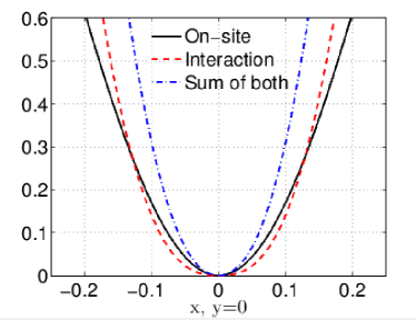
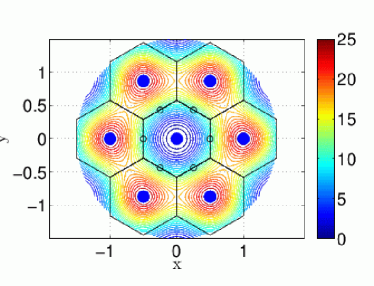
Figure 11. Unrelaxed potential computations. Parameter values: $r_{cut}=\sqrt{3}\sigma$, $\sigma=1$, $M=25$,$\epsilon=0.1$ and $U_{0}=2$. Left: unrelaxed potential functions as seen by a $\mathbf{K}$ atom moving in the $(1,0)^{T}$ crystallographic direction in a 2D $\mathbf{K}$-$\mathbf{K}$ sheet of the mica crystal lattice model. Right: energy contour lines as seen by the $\mathbf{K}$ atom at the origin moving in a 2D $\mathbf{K}$-$\mathbf{K}$ sheet of the mica crystal lattice model.

2.5. Numerical results

In this section we describe numerical results showing propagating discrete breather, kink and horseshoe wave solutions in an open lattice. Periodic boundary conditions can also be imposed. Open lattice simulation allows atoms to be ejected by the propagating waves at the edge of the lattice, which has possibly relevance to the experiment by Russell [22].

With zero initial velocities (momentum) and all $\mathbf{K}$ atoms being placed at the cell centres of the hexagonal lattice, the system (2.4)–(2.5) is in mechanical equilibrium, i.e. all forces of the system are equal to zero. The lattice is defined by $N_{x}$ atoms in the $x$ axis direction and an even number $N_{y}$ of atoms in the $y$ axis direction. The first atom is always placed at the origin $(0,0)$. The spacing between atoms in the $x$ direction is equal to the lattice constant $\sigma=1$ and in the $y$ direction, the lattice spacing between atoms is $h=\sqrt{3}/2\sigma$. The total number of atoms considered in the simulations is $N=N_{x}N_{y}-[N_{y}/2]$. In all simulations we use the Verlet method, as described above, with fixed time step $\tau=0.01$.

For the initial conditions, we consider imparting a non-zero velocity to one of the atoms while the rest of the lattice is kept at rest. The initial velocities of this atom in the $x$ and $y$ axis directions are indicated by $u_{x}^{0}$ and $u_{y}^{0}$, respectively. With different initial velocity kicks and with different parameter values $U_{0}$, we are able to observe different phenomena as discussed in the following sections. In addition, we will refer to the horizontal chain of atoms as the main chain of atoms along which the breather or kink solutions propagates, that is, the most of their energy has been localized on this chain. The final computational time is indicated by $T_{end}$.

By assigning half of the interaction potential energy to each atom in an interacting pair, while adding also the kinetic and potential energy values from the on-site potential, we can define an energy density function for each atom. Since the interaction potential may take negative values, we can normalize it. To see small scales better, we take the logarithm of the energy density function, that is

$$H_{log}=\log(H+|\min\{H\}|+1),$$

such that $H_{log}\geq{0}$. In all energy plots we plot $H_{log}$ and interpolate its values on uniform meshes for plotting purposes only.

2.5.1. Numerical results: propagating breather solutions

This subsection is devoted to the study of propagating discrete breather solutions. We perform numerical tests by exciting one atom in the system, i.e., by giving a single initial kick. We provide the impulse to the atom in the middle of the lattice with respect to the $y$ axis. Numerical results with $N_{x}=100$, $N_{y}=40$, $U_{0}=2$, $u_{x}^{0}=3$ and $u_{y}^{0}=0$ are shown in Fig. 12. We integrate in time until $T_{end}=80$. Figure 12 illustrates the propagation of the breather energy in time on a horizontal lattice chain in the $(1,0)^{T}$ crystallographic direction. We have excluded atoms at the boundaries from the plots due to high potential values at the boundaries. The breather in the $x$ axis direction is localized in space on about seven lattice sites and on about three lattice sites in the $y$ axis direction.

The initial kick has produced a highly localized quasi-one-dimensional breather solution. The excess energy of the kick produces phonons which spread into the lattice at higher velocities than the breather. In addition, the kick has produced a secondary breather solution with a lower energy propagating in the opposite direction. After some time, this breather solution elastically reflects from the boundary and follows the main breather solution. To illustrate that, we plot (in time after each $20$ time steps) the energy density function of atoms on the main horizontal chain along which the breather propagates, see the left plot of Fig. 13. We plot the atomic displacements in the $x$ axis direction of the same lattice chain in the right plot of Fig. 13. From the displacement plot we can conclude that the localized mode is an optical breather.

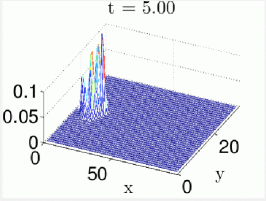
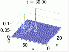
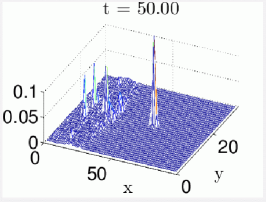
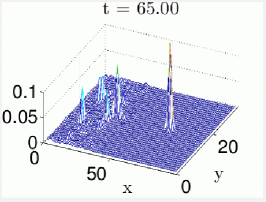
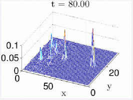
Figure 12. Evolution of the energy density function in time of the breather solution. $N_{x}=100$, $N_{y}=40$, $T_{end}=80$, $U_{0}=2$, $u_{x}^{0}=3$ and $u_{y}^{0}=0$.

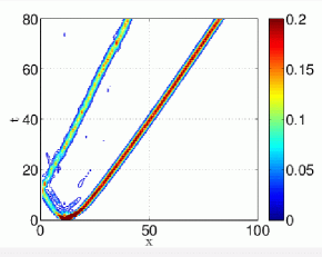
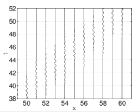
Figure 13. Short time simulation of a propagating breather. $N_{x}=100$, $N_{y}=40$, $T_{end}=80$, $U_{0}=2$, $u_{x}^{0}=3$ and $u_{y}^{0}=0$. Left: contour plot of the atomic energy density function on a horizontal lattice chain. Right: atomic displacements in the $x$ axis direction from their equilibrium positions in time on a horizontal lattice chain.

To test the lifespan of the breather solutions, we perform long time simulations with the same initial conditions and parameter values on a longer lattice, that is, on a long lattice strip: $N_{x}=6000$ and $N_{y}=40$. We integrate in time until $T_{end}=14000$. In the left plot of Fig. 14, we plot the energy density function of atoms after each $7000$ time steps on the main lattice chain in time. The result shows the long lifespan of propagating discrete breathers in crystal model at 0^∘K. The breather has propagated more than $5000$ lattice sites. The second curve in the left plot of Fig. 14 is due to the presence of the second propagating breather, see the description above. To see that these localized energies in the left plot of Fig. 14 are associated with the discrete breathers, we take snapshots of the energy density function at two distinct times from the simulation and show them in Fig. 15. To confirm the good energy conservation properties of the Verlet method, we have included in the right plot of Fig. 14 a graph of absolute relative error of the total energy in time. The graph shows that the total energy stays bounded for long integration times.

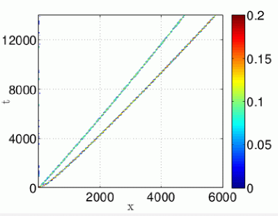
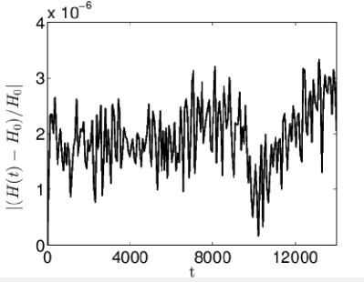
Figure 14. Long time simulation of propagating breather on a long strip lattice: $N_{x}=6000$, $N_{y}=40$, $T_{end}=14000$, $U_{0}=2$, $u_{x}^{0}=3$ and $u_{y}^{0}=0$. Left: energy density contour plot on a lattice line. Right: absolute relative error of total energy in time.

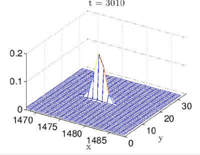
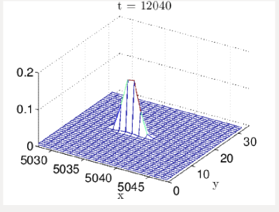
Figure 15. Snapshots of the energy density function of the propagating breather solution at two distinct times. Long strip lattice simulation: $N_{x}=6000$, $N_{y}=40$, $T_{end}=14000$, $U_{0}=2$, $u_{x}^{0}=3$ and $u_{y}^{0}=0$.

We can excite propagating discrete breathers for wide range of initial kick values. Taking smaller values for initial kicks leads to stationary breather solutions. For very small initial kick there is no localization and only phonons are produced. If we keep increasing the initial kick values, the kink solutions appear, which are the topic of next section.

Remark: Numerical simulations showed that with the same initial conditions but with larger values of $U_{0}$, the breather gets pinned to the lattice, but with smaller values of $U_{0}$ very distinctive horseshoe wave solutions appear, which we will discuss in Sec. 2.5.3. Recall that we control the relative strength of the potentials in dynamics with the parameter value $U_{0}$.

2.5.2. Numerical results: kink solutions

In this section we report on long lived kink solutions. For fixed value $U_{0}=2$ we keep increasing the initial velocity value of the kick. In the first numerical simulation, we consider a lattice with $N_{x}=100$ and $N_{y}=40$. The initial velocity kick values are $u_{x}^{0}=5.5$ and $u_{y}^{0}=0$. Such kicks produces a kink solution propagating on a horizontal chain of atoms. In Figure 16 we show evolution of kink’s energy in time. We integrate in time until $T_{end}=30$. Shortly before $25$ time units, the kink has approached the boundary and ejects two atoms from the lattice. That can be seen in the left plot of Fig. 17 where we plot the energy density function of atoms on the main chain along which the kink propagates, after each $10$ time steps in time. In the right plot of Fig. 17 we plot atomic displacements in the $x$ axis direction. Note the fundamental difference between breather and kink solutions. The kink solution is carried by the atoms from one unit cell to other, while a propagating breather passes through the lattice without atoms leaving their unit cells. Thus kink solutions may form vacancies inside the lattice as evident from the right plot of Fig. 17.

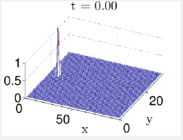
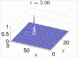
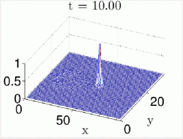
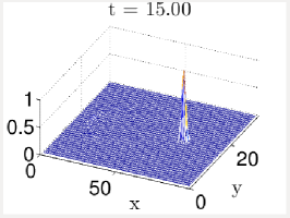
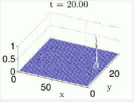
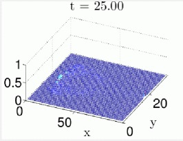
Figure 16. Evolution of the energy density function of the kink solution in time. $N_{x}=100$, $N_{y}=40$, $T_{end}=30$, $U_{0}=2$, $u_{x}^{0}=5.5$ and $u_{y}^{0}=0$.

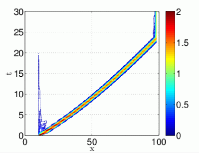
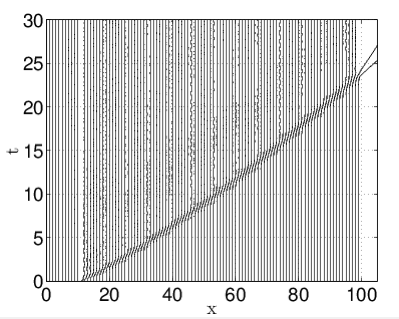
Figure 17. Short time simulation of a kink solution, with $N_{x}=100$, $N_{y}=40$, $T_{end}=30$, $U_{0}=2$, $u_{x}^{0}=5.5$ and $u_{y}^{0}=0$. Left: contour plot of the atomic energy density function on a horizontal lattice chain. Right: atomic displacements in the $x$ axis direction from their equilibrium positions in time on a horizontal lattice chain.

In Section 2.5.1 we demonstrated the long lifespan of propagating discrete breather solutions, see left plot of Fig. 14. We find that our model also supports long-lived kink solutions. For long-lived kink simulations, we consider long strip lattice: $N_{x}=2500$ and $N_{y}=40$. With the same parameter values and initial conditions we integrate in time until $T_{end}=1500$. In Figure 18, we plot the kink’s energy in time after each $750$ time steps of the main lattice chain. The kink has propagated over more than $2000$ lattice sites and has not collapsed during the whole computational time window.

What about the argument above that a kink should not be able to propagate in 2D? In these solutions the essential feature is that the “side wall” of the kink has zero energy - the atoms on the main chain have moved exactly $\sigma$ before and after the kink passes. So displacements across the wall is zero. If the wall was wider, then it would have finite energy, and we would not observe this phenomena.

Figure 18. Energy density function of a long time simulation of a propagating kink on a long strip lattice: $N_{x}=2500$, $N_{y}=40$, $T_{end}=1500$, $U_{0}=2$, $u_{x}^{0}=5.5$ and $u_{y}^{0}=0$.

Remark: If we keep the same initial condition but increase the value of $U_{0}$, the kink disappears. For a kink to appear again we have to increase the initial velocity kick value $u_{x}^{0}$. On the another hand if we keep the same initial condition but decrease the value of $U_{0}$, the kink disappears too. Instead horseshoe wave solutions appear, see Sec. 2.5.3.

2.5.3. Numerical results: horseshoe wave solutions

So far we have considered constant value of $U_{0}=2$. The parameter $U_{0}$ controls the relative strength between two potentials considered, i.e. the atom-atom interaction and the on-site potential. In this section we perform numerical study with smaller value of $U_{0}$, which lead to the observation of horseshoe wave solutions.

For this numerical test we consider a lattice: $N_{x}=100$ and $N_{y}=120$, and the same initial kicks which led to the observation of propagating breather solutions in Sec. 2.5.1, that is, $u_{x}^{0}=3.0$ and $u_{y}^{0}=0$. We integrate in time until $T_{end}=52$ with $U_{0}=0.1$. In Figure 19 we show the evolution of the energy density function in time. From the energy plots, we observe circular propagating wave spreading in all directions until it hits the boundaries.

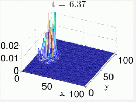
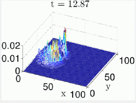
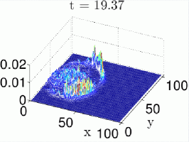
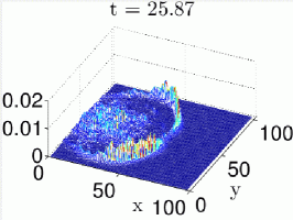
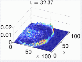
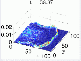
Figure 19. Evolution of the energy density function in time for the horseshoe wave solution. $N_{x}=100$, $N_{y}=120$, $T_{end}=52$, $U_{0}=0.1$, $u_{x}^{0}=3.0$ and $u_{y}^{0}=0$.

At fixed time we make a contour plot of the energy density function, see the left plot of Fig. 20. From this image it becomes evident that the wave adopts a horseshoe shape. We are interested in understanding the properties of the front wave of the horseshoe wave solutions. We find that the cross-section of the front wave is a breather solution. We consider a chain of atoms (assuming perpendicular to the front) shown by the dots in the left plot of Fig. 20 and show their energy density in time after each $13$ time steps in the right plot of Fig. 20. The particular chain of atoms is perpendicular to the $(1/2,\sqrt{3}/2)^{T}$ crystallographic lattice direction and makes $-30\,^{\circ}$ with the $x$ axis. The right plot of Fig. 20 confirms the propagating breather characteristics of the front wave of the horseshoe wave solution.

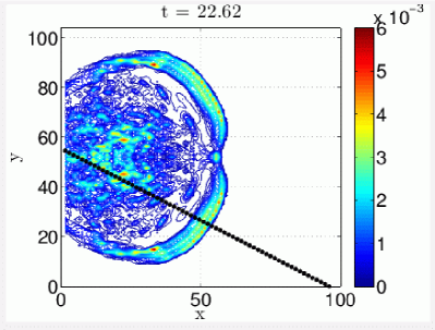
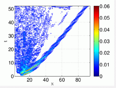
Figure 20. Contour plots of the energy density function. Left: over the whole domain at time $t=22.62$. Dark dots indicate a chain of atoms. Right: over the cross-section of the front wave in time, that is, energy of the atoms on the chain shown in the left plot. $N_{x}=100$, $N_{y}=120$, $T_{end}=52$, $U_{0}=0.1$, $u_{x}^{0}=3.0$ and $u_{y}^{0}=0$.

2.5.4. Numerical results: in-line collisions

In this section we study in-line breather-breather, kink-kink and breather-kink collisions. To initiate both types of wave propagations, we excite two atoms in the lattice, that is, we give initial velocity kicks to two atoms on the same lattice chain of atoms. The left atom initial velocity kick is $u_{x}^{0}$ and $u_{y}^{0}$, and the right atom velocity kick is $u_{x}^{1}$ and $u_{y}^{1}$. We start with the rest of the lattice in its mechanical equilibrium state. In all the following numerical experiments, $N_{x}=200$ and $N_{y}=40$, $U_{0}=2$ and $u_{y}^{0}=u_{y}^{1}=0$.

For our first example we consider in-line breather-breather collision with initial kicks: $u_{x}^{0}=1$ and $u_{x}^{1}=-3.5$. Integration in time is performed until $T_{end}=120$, see Fig. 21. In the left plot of Fig. 21, we show energy density function in time after each $20$ time steps on the main chain of atoms. Both kicks have produced two propagating breather solutions moving in opposite directions. All four breathers have different energies as can be seen by the colours. After $60$ time units, two middle breathers collide and pass through each other, exchanging some energy in the process. Evidently, the breather coming from the left has lost some of its initial velocity and propagates slower. The displacement plot of atoms in the $x$ axis direction during the collision can be seen in the right plot of Fig. 21.

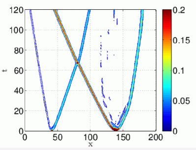
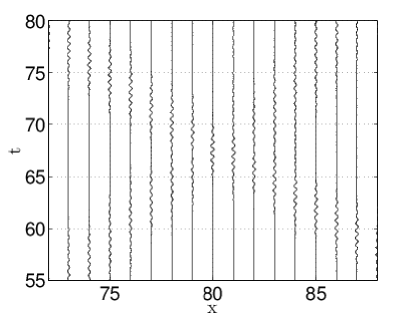
Figure 21. In-line collision of two propagating breathers. $N_{x}=200$, $N_{y}=40$, $T_{end}=120$, $U_{0}=2$, $u_{y}^{0}=u_{y}^{1}=0$, $u_{x}^{0}=1$ and $u_{x}^{1}=-3.5$. Left: contour plot of the energy density function in time on the lattice line. Right: atomic displacement plot in the $x$ axis direction on the lattice line during the collision.

For our second example, we consider in-line kink-kink collisions with initial kicks of $u_{x}^{0}=5.25$ and $u_{x}^{1}=-5.5$. Integration in time is carried out until $T_{end}=60$, see Fig. 22. In the left plot of Fig. 22 we show the energy density function in time after each $10$ time steps on the main chain of atoms where kinks propagate. Both kicks have produced a kink moving towards each other. Around $15$ time units, two kinks collide and re-appear after the collision, see the displacement plot of Fig. 22 on the right. Interestingly, when the kinks approach their initial locations, they fill the vacancies (stationary anti-kinks) left behind, and this scattering creates breather solutions.

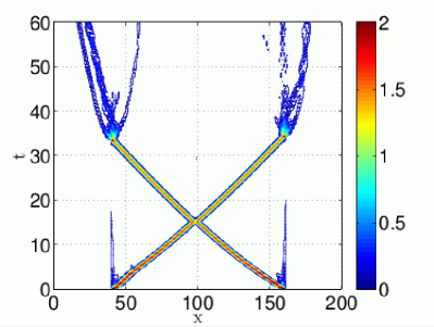
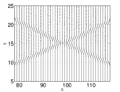
Figure 22. In-line collision of two kinks. $N_{x}=200$, $N_{y}=40$, $T_{end}=60$, $U_{0}=2$, $u_{y}^{0}=u_{y}^{1}=0$, $u_{x}^{0}=5.25$ and $u_{x}^{1}=-5.5$. Left: contour plot of the energy density function in time on the lattice line. Right: atomic displacement plot in the $x$ axis direction on the lattice line.

To illustrate this phenomenon more clearly, we perform additional tests on the same lattice but with the second atom’s initial kick taken to have opposite sign, i.e. $u_{x}^{0}=5.5$ and $u_{x}^{1}=5.25$, see Fig. 23. Now both kinks propagate in the same direction. When the kink on the left approaches the vacancy (anti-kink) created by the kink on the right, the kink fills the vacancy and creates a stationary as well as propagating breather solutions moving in both directions. The vacancy filling can be clearly seen in the right plot of Fig. 23, where we show the displacement of atoms in the $x$ axis direction of the atoms on the main horizontal lattice chain. This numerical test shows that propagating breather solutions can not only be created by the kicks but also by kink solutions filling vacancies (colliding with anti-kinks) in the crystal lattice.

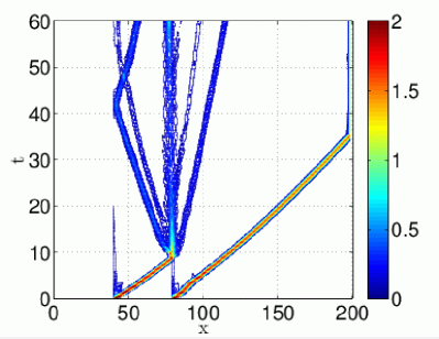
Figure 23. In-line collision of two kinks. $N_{x}=200$, $N_{y}=40$, $T_{end}=60$, $U_{0}=2$, $u_{y}^{0}=u_{y}^{1}=0$, $u_{x}^{0}=5.5$ and $u_{x}^{1}=5.25$. Left: contour plot of the energy density function in time on the lattice line. Right: atomic displacement plot in the $x$ axis direction on the lattice line.

For our final in-line collision experiment, we consider breather-kink collision with initial velocity kicks $u_{x}^{0}=3.5$ and $u_{x}^{1}=-5.5$. We integrate in time until $T_{end}=60$ and illustrate the numerical results in Fig. 24. In the left plot of Fig. 24, we show the energy density function in time after each $10$ time steps on the main chain of atoms where the breather and kink propagate. The kick on the left has produced two breather solutions propagating in opposite directions, and the kick on the right has produced a kink solution moving to the left towards the breather solutions. After around $30$ time units, the breather and kink solutions collide and pass through each other. Later in time the kink passes through the second breather solution propagating in the same direction. The first collision is also illustrated by the displacement plot in Fig. 24 on the right. These results suggest that breather and kink solutions can easily coexist in our model of a crystal lattice.

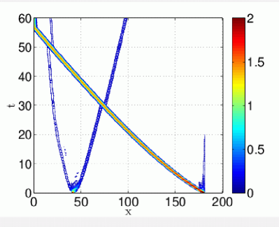
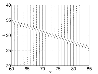
Figure 24. In-line collision of breather and kink solutions. $N_{x}=200$, $N_{y}=40$, $T_{end}=60$, $U_{0}=2$, $u_{y}^{0}=u_{y}^{1}=0$, $u_{x}^{0}=3.5$ and $u_{x}^{1}=-5.5$. Left: contour plot of the energy density function in time on the lattice line. Right: atom displacement plot in the $x$ axis direction on the lattice line.

2.5.5. Numerical results: fully 2D effects

So far, except for the horseshoe wave solutions, see Sec. 2.5.3, all numerical examples have addressed the quasi-one-dimensional nature of propagating discrete breather and kink solutions. In this section we demonstrate full 2D effects of the numerical solutions by considering kink-kink and breather-kink collisions on adjacent chains of atoms, and breather-breather collision at $60\,^{\circ}$ angle to each other.

If the kink solutions of our 2D model were truly one-dimensional, we would expect no interactions between two kink solutions in kink-kink collisions, with the kinks travelling in opposite directions along adjacent chains of atoms. This is not the case, as can be seen in Fig. 25. The lattice, parameter values and initial kicks are identical to the in-line kink-kink collision experiment in Sec. 2.5.4.

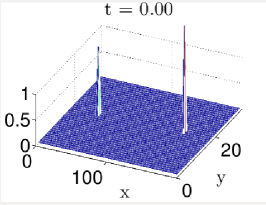
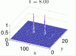
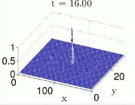
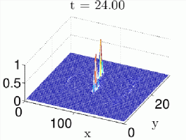
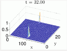
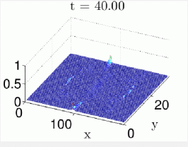
Figure 25. Energy density evolution in time of two kink collision on adjacent chains of atoms. $N_{x}=200$, $N_{y}=40$, $T_{end}=40$, $U_{0}=2$, $u_{y}^{0}=u_{y}^{1}=0$, $u_{x}^{0}=5.25$ and $u_{x}^{1}=-5.5$.

In Figure 25, we show the evolution of the energy density function in time. The localized energy peaks are associated with the two kinks propagating towards each other on adjacent lattice chains. At $t\approx 16$, the two kinks collide and change their propagation directions after collision. After a complicated collision region, the right kink eventually propagates in the $(1/2,-\sqrt{3}/2)^{T}$ crystallographic lattice direction, while the left kink propagates in the $(1/2,\sqrt{3}/2)^{T}$ crystallographic lattice direction. Once each kink has approached the upper or lower boundary they eject one atom from the lattice. This example of collisions shows a new scattering phenomena in a 2D lattice model which has no counterpart in 1D lattice models. It shows that there is at least weak coupling between kink solution and atoms on adjacent chains.

To understand better the events taking place during the kink-kink collision on adjacent lines, we consider scatter plots of atoms in time during the collision, see Fig. 26. We zoom into the lattice area where the collision takes place. Darker colours indicate higher energy density function values. The first plot shows kinks approaching each other while the final plot shows kink solutions, already fully developed, propagating in the different crystallographic lattice directions. From Figure 26 it becomes evident that the two kinks, in fact, passed by each other. Due to the weak coupling between kinks on adjacent lines, the collision has destabilized the kinks by inducing large displacements in the $y$ axis direction. This induced instability causes the kinks to change their propagation directions. This may suggest that long-lived kink solutions may only exist in completely idealized settings.

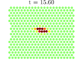
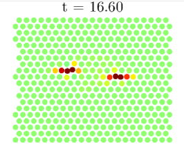
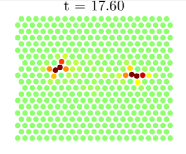
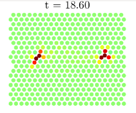
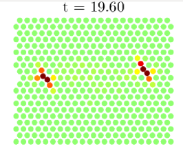
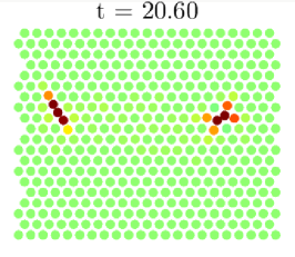
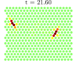
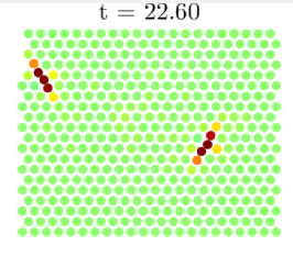
Figure 26. Snapshots of scatter plots of atoms in time of two kink collision on adjacent chains of atoms. $N_{x}=200$, $N_{y}=40$, $T_{end}=40$, $U_{0}=2$, $u_{y}^{0}=u_{y}^{1}=0$, $u_{x}^{0}=5.25$ and $u_{x}^{1}=-5.5$.

In general, results of collisions do not always follow the same pattern. The outcome will depend on the energy, velocity and phase of propagating localized modes. We illustrate that with a counter example of two kink collision on adjacent chains of atoms, see Fig. 27. For this experiment we consider a twice larger lattice: $N_{x}=400$ and $N_{y}=40$, and initial kick values $u_{x}^{0}=5.3$ and $u_{x}^{1}=-5.4$. In the left plot of Fig. 27 we show energy density function in time of atoms on the main chain of the kink moving from the left, and in the right plot of Fig. 27 we show energy density function in time of atoms on the main chain of the kink moving from the right. Integration in time is carried out until $T_{end}=100$ and results are illustrated after each $20$ time steps. After around $50$ time units, the two kinks collide, lose some of their initial velocity and continue to propagate, but slower. This suggest that both kinks have lost some energy during the collision to the lattice in the form of phonons. In addition, plots of Fig. 27 confirm that there is some energy associated to the kink solutions on adjacent chains of atoms. Notice the change of the slopes in those energies after the collision.

Figure 27. Two kink collision on adjacent chains of atoms. $N_{x}=400$, $N_{y}=40$, $T_{end}=100$, $U_{0}=2$, $u_{y}^{0}=u_{y}^{1}=0$, $u_{x}^{0}=5.3$ and $u_{x}^{1}=-5.4$. Left: contour plot of the energy density function in time on the main chain of atoms of the kink on the left. Right: contour plot of the energy density function in time on the main chain of atoms of the kink on the right.

The destabilizing effects due to lateral displacements of atoms on the main chain where the mode propagates is not only present in kink-kink collisions, but also in breather-kink and breather-breather collisions. Recall that there are almost zero lateral displacements on the main chain of atoms where the breather or kink propagates in an idealized setting. To support our claims we present numerical experiments of breather-kink collision on adjacent lines and breather-breather collision at $60\,^{\circ}$ angles to each other.

We consider the same breather-kink collision example from Sec. 2.5.4, but on adjacent chains and on the larger (x2) lattice: $N_{x}=400$ and $N_{y}=40$. We integrate in time until $T_{end}=140$ and plot the associated energy density of atoms in both chains in time after each $20$ time steps in Fig. 28. Compare Figs. 28 and 24. We find that the kink has scattered the breather solution during the collision into the remaining lattice, see the left plot of Fig. 28, but the collision itself has not affected the kink solution, see the right plot of Fig. 28. This example once again illustrates 2D effects.

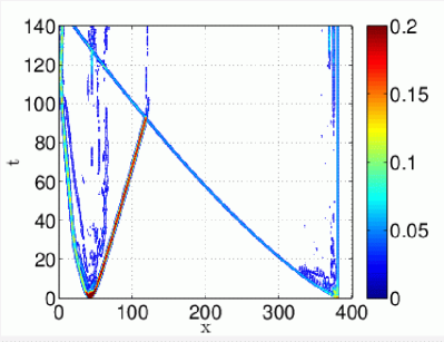
Figure 28. Breather-kink collision on adjacent chains of atoms. $N_{x}=400$, $N_{y}=40$, $T_{end}=140$, $U_{0}=2$, $u_{y}^{0}=u_{y}^{1}=0$, $u_{x}^{0}=3.5$ and $u_{x}^{1}=-5.5$. Left: contour plot of the energy density function in time on the main chain of the breather solution. Right: contour plot of the energy density function in time on the main chain of atoms of the kink solution.

In the final example of this section we consider a breather-breather collision at a $60\,^{\circ}$ angles to each other. In this example we give a kick to one atom in the left lower area and a kick to one atom in the right upper area of the lattice: $N_{x}=200$ and $N_{y}=100$. The initial kick values are $u_{x}^{0}=1$ and $u_{y}^{0}=0$, and $u_{x}^{1}=-2.5\cos(\pi/3)$ and $u_{y}^{0}=-2.5\sin(\pi/3)$. We carry out integration in time until $T_{end}=400$. We illustrate the collision area in time with snapshot scatter plots of atoms in Fig 29. Darker colours indicate higher energy density function values. The first breather propagates from left to right on the horizontal lattice chain and the second breather propagates downwards on the $(1/2,\sqrt{3}/2)^{T}$ crystallographic lattice chain. During the collision both breathers merge into one stationary breather localized on the $(1/2,-\sqrt{3}/2)^{T}$ crystallographic lattice chain. Depending on the breather’s energies, velocity and phase, we have observed breathers merging into one stationary or one propagating breather, passing through each other or changing their propagation directions.

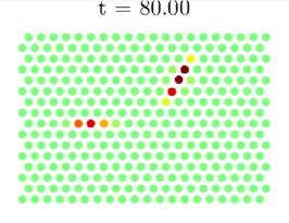
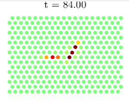
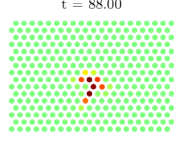
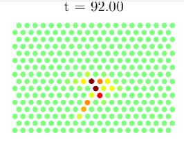
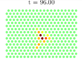
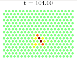
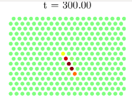
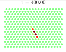
Figure 29. Snapshots of scatter plots of atoms in time of two breather collision at $60\,^{\circ}$ angle to each other. $N_{x}=200$, $N_{y}=100$, $T_{end}=400$, $U_{0}=2$, $u_{x}^{0}=1$, $u_{y}^{0}=0$, $u_{x}^{1}=-2.5\cos(\pi/3)$ and $u_{y}^{0}=-2.5\sin(\pi/3)$.

The results presented above can be summarized by one consideration. The additional degree of freedom introduces three crystallographic lattice directions, in contrast to 1D models on which localized modes can travel, thus introducing additional richness into interaction properties. Due to the quasi-one-dimensional nature of travelling modes, lateral displacements of atoms on the main chain induced through interactions may destabilize propagating modes. At the same time, the additional degree of freedom allows us to observe new wave phenomena such as horseshoe wave solutions from Sec. 2.5.3 and the 2D multi-kink solutions of the following section.

2.5.6. Numerical results: 2D multi-kink solution

In this section we present a brief example of a 2D coupled-kink solution. This is a multiple kink-like mode where two or more kinks travel together side-by-side with the front perpendicular to the direction of travel. The initial formation of such a solution was observed from a kink-kink collision experiment at $60\,^{\circ}$ angle to each other which we demonstrate here. Consider the experiment of breather-breather collision at $60\,^{\circ}$ angle to each other from Sec. 2.5.5 but with initial kick values $u_{x}^{0}=5.5$, $u_{y}^{0}=0$, $u_{x}^{1}=-5.25\cos(\pi/3)$ and $u_{y}^{0}=-5.25\sin(\pi/3)$. These particular initial kick values produce two kink solutions. The first kink propagates from left to right on a horizontal lattice chain in $(1,0)^{T}$ crystallographic lattice direction and the second kink propagates downwards on the $(1/2,\sqrt{3}/2)^{T}$ crystallographic lattice chain, see Fig. 30. During the collision both kinks merge together and form a stable double-kink solution propagating to the right on two adjacent chains of atoms.

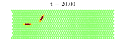
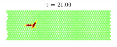
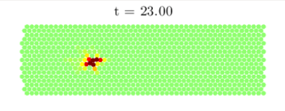
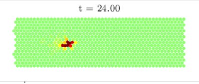
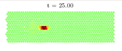
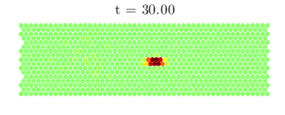
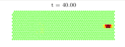
Figure 30. Snapshots of scatter plots of atoms in time of two kink collision at $60\,^{\circ}$ angle to each other. $N_{x}=200$, $N_{y}=100$, $T_{end}=40$, $U_{0}=2$, $u_{x}^{0}=5.5$, $u_{y}^{0}=0$, $u_{x}^{1}=-5.25\cos(\pi/3)$ and $u_{y}^{0}=-5.25\sin(\pi/3)$.

The observation of the stable formation of a double-kink solution, Fig. 30, led us to consider coupled multi-kink simulations, that is, by considering multiple kicks of neighbouring atoms in the $y$ axis direction. For this experiment we consider a lattice: $N_{x}=1200$ and $N_{y}=40$, and equal initial kick values $u_{x,i}^{0}=5.5$, $u_{y,i}^{0}=0$ on seven atoms, i.e. $i=1,\dots,{7}$, see the top left plot of Fig. 31 at $t=0$. Importantly, non-equal initial kick values may lead to scattering of kinks in all three crystallographic lattice directions. We integrate in time until $T_{end}=400$. In Figure 31, we show snapshots of scatter plots of atoms in time at locations of maximal energy density function in space indicated by the $x$ coordinate. Numerical results show that the structure of multiple kink solutions has propagated more than $1000$ lattice sites and suggest that such type of structures may be long-lived in idealized settings. Interestingly, the same type of initial kick values did not lead to the formation of joint breather solutions.

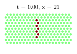
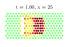
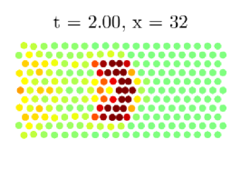
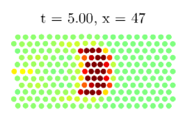
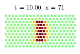
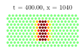
Figure 31. Snapshots of scatter plots of atoms in time of a multi-kink solution. $N_{x}=1200$, $N_{y}=40$, $T_{end}=400$, $U_{0}=2$, $u_{x,i}^{0}=5.5$ and $u_{y,i}^{0}=0$, where $i=1,\dots,{7}$.

3. Conclusions and Future Plans

We have confirmed and much extended the calculations of Marín et al. showing the existence of long lived quasi-one-dimensional discrete breathers in hexagonal lattices. A further paper using a more conventional particle-particle potential will discuss such solutions in more detail [2]. The present model also displays long-lived quasi-one-dimensional discrete kinks in our model mica lattice. However as discussed in [2], this type of solution is more sensitive to the details of the inter-atomic potentials considered, and other models give much shorter kink lifetimes. It remains to be seen if existing or novel materials can exhibit such kinks in physical situations.

We show that the kinks and breathers exhibit a typical rich variety of phenomena on collision along a mutual line of quasi-one-dimensional travel. In addition we demonstrate fully 2D collision phenomena for the first time, for kinks/breathers travelling on adjacent lines or at $60^{\circ}$ angles to each other. Moreover we observe a new type of spreading shock wave, the horseshoe wave, with a breather profile. In view of the many different possible outcomes of such collisions, a more systematic and quantitative study is required for the future.

We have not discussed thermal or other random perturbations to the model in the present paper, some brief studies will be reported in [2]. In at attempt to understand ejection and sputtering in such models, it would be important to model surface forces properly. In general a more serious attempt to fit model parameters to real MD data from mica is required. A further study should concentrate on the effects of longer-range forces and how these effect breather and kink lifetimes.

A multi-core and HPC version of the code will be an important next step, as this is necessary for long runs, to establish the maximum lifetimes of breathers and kinks under ideal conditions. In the full 2D model it would be interesting to investigate scattering of breathers and kinks with vacancies, dislocations and inclusions, etc., to generalise the 1D studies such as [3]. Adding temperature effects to this sort of study would be important.

The present study shows a variety of new interesting phenomena, but the field of 2D breathers and kinks is still in its infancy, with much still to be done, in both theoretical and experimental areas.

References

- [1] M. P. Allen and D. J. Tildesley. Computer Simulation of Liquids. Oxford science publications. Oxford University Press, USA, 1989.
- [2] Janis Bajars, J. Chris Eilbeck, and Ben Leimkuhler. Nonlinear propagating localized modes in a 2d hexagonal crystal lattice. preprint, 2014.
- [3] J. Cuevas, C. Katerji, J. F. R. Archilla, J. C. Eilbeck, and F. M. Russell. Influence of moving breathers on vacancies migration. Phys. Lett. A, 315:364–371, 2003.
- [4] Q. Dou, J. Cuevas, J. C. Eilbeck, and F. M. Russell. Breathers and kinks in a simulated crystal experiment. Discrete and Continuous Dynamical Systems - Series S, 4:1107–1118, 2011.
- [5] D. B. Duncan, J. C. Eilbeck, H. Feddersen, and J. A. D. Wattis. Solitons on lattices. Physica D, 68:1–11, 1993.
- [6] J. C. Eilbeck. Numerical simulations of the dynamics of polypeptide chains and proteins. In C Kawabata and A. R. Bishop, editors, Computer Analysis for Life Science, pages 12–21, Tokyo, 1986. Ohmsha.
- [7] J. C. Eilbeck, P. S. Lomdahl, and A. C. Scott. Soliton structure in crystalline acetanilide. Phys. Rev. B, 30:4703–4712, 1984.
- [8] J. C. Eilbeck, P. S. Lomdahl, and A. C. Scott. The discrete self-trapping equation. Physica D, 16:318–338, 1985.
- [9] H. Feddersen. Solitary wave solutions to the discrete nonlinear Schrödinger equation, pages 159–167. Springer, 1991.
- [10] S. Flach and C.R. Willis. Discrete breathers. Physics Reports, 295:181–264, 1998.
- [11] Sergej Flach. Discrete breathers in a nutshell. Nonlinear Theory and Its Applications, IEICE, 3:12–26, 2012.
- [12] A. K. Geim and I. V. Grigorieva. Van der Waals heterostructures. Nature, 499:419–425, 2013.
- [13] B. Leimkuhler and S. Reich. Simulating Hamiltonian Dynamics. Cambridge University Press, 2004.
- [14] R.S. MacKay and S. Aubry. Proof of existence of breathers for time-reversible or hamiltonian networks of weakly coupled oscillators. Nonlinearity, 7:1623–1643, 1994.
- [15] N. Manton and P. Sutcliffe. Topological Solitons. Cambridge Universty Press, 2004.
- [16] J. L. Marín, J. C. Eilbeck, and F. M. Russell. Localised moving breathers in a 2-d hexagonal lattice. Phys. Lett. A, 248:225–229, 1998.
- [17] J. L. Marín, J. C. Eilbeck, and F. M. Russell. 2-D Breathers and applications, pages 293–306. Springer, 2000.
- [18] J. L. Marín, F. M. Russell, and J. C. Eilbeck. Breathers in cuprate superconductor lattices. Phys. Letts. A, 281:225–229, 2001.
- [19] A. A. Ovchinnikov. Localized long-lived vibrational states in molecular crystals. Soviet Physics JETP, 30:147–150, 1970.
- [20] Michel Peyrard and Martin D. Kruskal. Kink dynamics in the highly discrete sine-gordon system. Physica D: Nonlinear Phenomena, 14:88––102, 1984.
- [21] F. M. Russell and D. R. Collins. Lattice-solitons and non-linear phenomena in track formation. Rad. Meas., 25:67–70, 1995.
- [22] F. M. Russell and J. C. Eilbeck. Evidence for moving breathers in a layered crystal insulator at 300k. Phys. Letts. A, 78:10004, 2007.
- [23] A. C. Scott and L. MacNeil. Binding energy versus nonlinearity for a small stationary soliton. Phys. Lett. A, 98:87–88, 1983.
- [24] Y. Yang, W. S. Duan, L. Yang, J. M. Chen, and M. M. Lin. Rectification and phase locking in overdamped two-dimensional Frenkel-Kontorova model. Europhysics Letters, 93(1):16001, 2011.