Spin and energy currents in integrable and nonintegrable spin- chains:
A typicality approach to real-time autocorrelations
Abstract
We use the concept of typicality to study the real-time dynamics of spin and energy currents in spin- models in one dimension and at nonzero temperatures. These chains are the integrable XXZ chain and a nonintegrable modification due to the presence of a staggered magnetic field oriented in direction. In the framework of linear response theory, we numerically calculate autocorrelation functions by propagating a single pure state, drawn at random as a typical representative of the full statistical ensemble. By comparing to small-system data from exact diagonalization (ED) and existing short-time data from time-dependent density matrix renormalization group (tDMRG), we show that typicality is satisfied in finite systems over a wide range of temperature and is fulfilled in both, integrable and nonintegrable systems. For the integrable case, we calculate the long-time dynamics of the spin current and extract the spin Drude weight for large systems outside the range of ED. We particularly provide strong evidence that the high-temperature Drude weight vanishes at the isotropic point. For the nonintegrable case, we obtain the full relaxation curve of the energy current and determine the heat conductivity as a function of magnetic field, exchange anisotropy, and temperature.
pacs:
05.60.Gg, 71.27.+a, 75.10.JmI Introduction
The concept of typicality gemmer2003 ; goldstein2006 ; reimann2007 ; popescu2006 ; white2009 ; hams2000 ; bartsch2009 ; sugiura2012 ; elsayed2013 ; steinigeweg2014-1 ; steinigeweg2014-2 states that a single pure state can have the same properties as the full statistical ensemble. This concept is not restricted to specific states and applies to the overwhelming majority of all possible states, drawn at random from a high-dimensional Hilbert space. In the cleanest realization, even a single eigenstate of the Hamiltonian may feature the properties of the full equilibrium density matrix, assumed in the well-known eigenstate thermalization hypothesis deutsch1991 ; srednicki1994 ; rigol2008 . The notion of property is manifold in this context and also refers to the expectation values of observables. Remarkably, typicality is not only a static concept and includes the dynamics of expectation values bartsch2009 . Recently, it has become clear that typicality even provides the basis for powerful numerical approaches to the dynamics of quantum many-particle systems at nonzero temperatures hams2000 ; elsayed2013 ; steinigeweg2014-1 ; steinigeweg2014-2 . These approaches are in the center of this paper.
Understanding relaxation and transport dynamics in quantum many-body systems is certainly one of the most desired and ambitious aims of condensed-matter physics and experiencing an upsurge of interest in recent years, both experimentally and theoretically. On the one hand, the advent of ultracold atomic gases raises challenging questions about the equilibration and thermalization in isolated many-particle systems cazalilla2010 , including the existence, origin, or speed of relaxation processes in the absence of any external bath. On the other hand, future information technologies such as spintronics call for a deeper insight into transport dynamics of quantum degrees of freedom such as spin excitations. Spin transport in conventional nano-systems appelbaum2007 ; tombros2007 ; stern2008 ; kuemmeth2008 is inevitably linked to the dynamics of itinerant charge carriers. In contrast, Mott-insulating quantum magnets allow for pure spin currents and thus open new perspectives in quantum transport. In the past decade, magnetic transport in one-dimensional quantum magnets has attracted considerable attention because of the discovery of very large magnetic heat-conduction sologubenko2000 ; hess2001 ; hlubek2010 and long nuclear magnetic relaxation times thurber2001 ; kuehne2010 . Genuine spin transport, however, still remains to be observed in experiments and particularly its classification in terms of ballistic or diffusive propagation is an issue of ongoing experimental research maeter2012 ; xiao2014 .
The theoretical study of transport in low-dimensional quantum magnets has a long and fertile history. Amongst all questions, the dissipation of currents is a key issue and has been investigated extensively at zero momentum and frequency in connection with the linear-response Drude weight zotos1997 ; kluemper2002 ; shastry1990 ; zotos1999 ; benz2005 ; prosen2011 ; prosen2013 ; narozhny1998 ; heidrichmeisner2003 ; heidrichmeisner2007 ; herbrych2011 ; steinigeweg2013 ; fujimoto2003 . The Drude weight is the nondissipating part of the current autocorrelation function and, if existent, indicates a ballistic channel close to equilibrium. While in generic nonintegrable systems it is commonly expected that Drude weights do not exist in the thermodynamic limit heidrichmeisner2003 , the picture is different and more complicated in integrable systems: Since an overlap of currents with the macroscopic number of conserved quantities is probable, Drude weights are expected to exist. But this overlap is not necessarily finite for all model parameters and Drude weights can vanish in the thermodynamic limit. In this context, an important example is the antiferromagnetic and anisotropic Heisenberg (XXZ) spin- chain. This chain is studied in the present paper. It is a fundamental model for the magnetic properties of interacting electrons in low dimensions. It is not only relevant to the physics of one-dimensional quantum magnets johnston2000 but also to physical questions in a much broader context trotzky2007 ; gambardella2006 ; kruczenski2004 ; kim1996 .
In the XXZ spin- chain, the heat current is strictly conserved for all values of the exchange anisotropy zotos1997 ; kluemper2002 and energy flows through a ballistic channel only. This type of flow is at the heart of the colossal heat conduction observed experimentally in almost ideal material realizations of the model sologubenko2000 ; hess2001 ; hlubek2010 . In contrast, the spin current is not strictly conserved and the existence of a spin Drude weight is a demanding problem, resolved only partially despite much effort. At zero temperature, , early work shastry1990 showed that the spin Drude weight is nonzero in the gapless regime (metal) but zero in the gapped regime (insulator). Bethe-Ansatz solutions zotos1999 ; benz2005 support a qualitatively similar picture at nonzero temperatures, , but with a disagreement at the isotropic point . Recent progress in combining quasi-local conservation laws and Mazur’s inequality has lead to a rigorous lower bound to the spin Drude weight in the limit of high temperatures prosen2011 ; prosen2013 . This bound is very close to the Bethe-Ansatz solution but still allows for a vanishing Drude weight at .
Numerically, a large variety of sophisticated methods has been applied to transport and relaxation dynamics in the anisotropic Heisenberg spin- chain, including full exact diagonalization (ED) narozhny1998 ; heidrichmeisner2003 ; heidrichmeisner2007 ; herbrych2011 ; steinigeweg2013 ; fabricius1998 ; steinigeweg2009 ; steinigeweg2011-1 , Lanczos methods prelovsek2013 ; mierzejewski2010 ; steinigeweg2012-1 , quantum Monte-Carlo techniques alvarez2002 ; grossjohann2010 , as well as time-dependent density matrix renormalization group (tDMRG) approaches to the real-time dynamics of wave packets or correlators langer2009 ; jesenko2011 ; karrasch2012 ; karrasch2013-1 ; karrasch2013-2 ; huang2013 ; karrasch2014-1 ; karrasch2014-2 and to the solution of the Lindblad quantum master equation prosen2009 ; znidaric2011 . The overwhelming majority of results for the spin Drude weight, however, is only available from ED and tDMRG. Since ED is at present restricted to chains of length , the long-time/low-frequency limit is still governed by finite-size effects and intricate extrapolation schemes to the thermodynamic limit have been invoked, with different results depending on details. Such details are using even or odd herbrych2011 and choosing grand-canonical and canonical ensembles karrasch2013-1 . Clearly, these details should be irrelevant in the thermodynamic limit. Alternatively, tDMRG is exceedingly more powerful w.r.t. system size and chains of length are accessible. But still the method is confined to a maximum time scale depending on the exchange anisotropy karrasch2012 ; karrasch2013-1 ; karrasch2014-1 ; karrasch2014-2 . Even though there is an ongoing progress to increase this time scale, it is at present too short for a reliable extraction of the spin Drude weight at the isotropic point karrasch2013-1 , which is both, experimentally relevant and theoretically most challenging. In this situation, typicality can provide a fresh numerical perspective steinigeweg2014-1 .
Much less is known on transport dynamics apart from the mere existence of Drude weights. For spin transport at , steady-state bath scenarios prosen2009 ; znidaric2011 and classical simulations alcantarabonfim1992 ; gerling1993 ; steinigeweg2012-2 suggest super-diffusive dynamics in the limit of high temperatures, while bosonization predicts diffusion at low but nonzero temperatures sirker2009 . At , signatures of diffusion have been observed also at high temperatures in different approaches prosen2009 ; znidaric2011 ; steinigeweg2012-2 ; steinigeweg2011-1 ; steinigeweg2011-2 ; steinigeweg2010 (see Ref. karrasch2014-1, for a discussion of the limit ). Diffusion of heat, however, necessarily requires integrability-breaking perturbations. For nonintegrable problems, perturbation theory is the only analytical technique available but hard to perform in the thermodynamic limit jung2006 ; jung2007 . The perturbative regime of small integrability-breaking is further challenging for numerical methods since dynamics is slow and physically relevant time scales are long. These long time scales are a challenge for tDMRG and, due to finite-size effects, also for ED. Thus, typicality may complement both numerical methods in this demanding regime.
In this paper, we use the concept of typicality to study the real-time dynamics of spin and energy currents in integrable and nonintegrable spin- chains at nonzero temperatures. In this way, we extend our previous work in Ref. steinigeweg2014-2, to energy transport and nonintegrable systems as well. Within the framework of linear response theory, we numerically obtain autocorrelation functions from the propagation of a single pure state, drawn at random as a typical representative of the full statistical ensemble. By comparing to small-system data from ED and existing short-time data from tDMRG, we show that typicality is satisfied in finite systems down to low temperatures and holds in both, integrable and nonintegrable systems. In particular, we demonstrate two numerical advantages of typicality: First, for integrable systems, we can calculate the long-time dynamics and extract the Drude weight for large systems outside the range of ED. Thus, typicality improves the reliability of finite-size scaling. Second, for nonintegrable systems, we can obtain the full relaxation curve for large systems with little finite-size effects on the physically relevant time scale. Hence, typicality provides also the basis for determining the dc conductivity in the regime of small integrability-breaking model parameters without using any fits/extrapolations. Both advantages yield significant progress in the numerical investigation of spin and energy dynamics in particular and of other observables in a much broader context.
This paper is structured as follows: In Sec. II we first introduce the two models studied, namely, the integrable XXZ spin- chain and a nonintegrable version due to the presence of a staggered magnetic field oriented in direction. In this Sec. we also define the spin and energy currents, as well as their time-dependent autocorrelation functions, and we discuss symmetries. The next Sec. III is devoted to the concept of dynamical typicality and the closely related numerical technique used throughout this paper. Then we turn to our results: In Sec. IV we focus on spin-current dynamics in the integrable model and study the spin Drude weight as a function of anisotropy and temperature. In the following Sec. V we extend our study in two directions: the nonintegrable model and the dynamics of the energy current. In this Sec. we analyze the dependence of the dc conductivity on magnetic field, anisotropy, and temperature. The last Sec. VI closes with a summary and draws conclusions.
II Models, Currents, and Autocorrelations
II.1 Integrable Model
In this paper we investigate the antiferromagnetic XXZ spin- chain. We employ periodic boundary conditions and write the well-known Hamiltonian ()
| (1) |
as a sum over the local energy
| (2) |
, are the components of spin- operators at site and is the total number of sites. is the antiferromagnetic exchange coupling constant and is the exchange anisotropy in direction. For , the model in Eq. (1) has no gap and an antiferromagnetic ground state; for , a gap opens and, for , the ground state becomes ferromagnetickolezhuk2004 ; karrasch2013-1 .
In general, Eq. (1) is integrable in terms of the Bethe Ansatz zotos1999 ; benz2005 and has several symmetries. Two commonly employed symmetries are the invariance under rotation about the axis, i.e., the conservation of , and translation invariance. Because of these symmetries, the longitudinal spin , and the momentum , are good quantum numbers. Therefore, the full Hilbert space with states consists of uncoupled symmetry subspaces with
| (3) |
states, where the largest subspaces have . In this paper we do not restrict ourselves to a specific choice of or and take into account all subspaces.
Since the longitudinal magnetization and energy are conserved, their currents are well defined operators and follow from the continuity equation
| (4) |
where is either the local magnetization, , or the local energy, , and is the corresponding local current. In case of magnetization, and the total current has the well-known form (see, e.g., the review in Ref. heidrichmeisner2007, )
| (5) |
where the subscript S indicates spin/magnetization for the remainder of this paper. This current commutes with the Hamiltonian only for anisotropy heidrichmeisner2007 . In the case of energy, and the total current can be written as steinigeweg2013
| (6) | |||||
where the subscript E indicates energy now. In contrast to the operators in Eqs. (1) and (5), the current in Eq. (6) acts on more than two neighboring sites and involves three adjacent sites. This current and the Hamiltonian commute with each other for all values of zotos1997 ; kluemper2002 . Both, energy and spin current share the good quantum numbers of the Hamiltonian.
II.2 Nonintegrable Model
To break the integrability of the model, we add to Eq. (1) the term
| (7) |
where is the strength of a staggered magnetic field oriented in direction. While this term does not change the above symmetries of the model, we have momentum , now and symmetry subspaces are twice as large as before.
Due to the form of , neither the definition of the spin current in Eq. (5) nor the definition of the energy current in Eq. (6) change. In general, is independent of any spatial profile of the magnetic field. But does not change because of the staggered profile of in Eq. (7). A homogenous magnetic field, for instance, yields a magnetothermal correction to the energy current heidrichmeisner2007 . Such a correction does not occur in our case. One important consequence of adding is a nonvanishing commutator
| (8) |
i.e., the energy current is not strictly conserved for finite values of and . Note that this commutator also leads to scattering rates , as discussed in more detail later and in Appendix B.
While the main physical motivation of adding a staggered magnetic field is both, breaking integrability and inducing current scattering, we do not intend to describe a specific experimental situation. Moreover, choosing as perturbation allows us to compare with existing results in the literature.
II.3 Autocorrelation Functions
Within the framework of linear response theory kubo1991 , we investigate spin and energy autocorrelation functions at inverse temperatures (),
| (9) | |||||
where the time argument of the operator has to be understood w.r.t. the Heisenberg picture, , and is the partition function. In the limit of high temperatures , the sum rules are given by and zotos1997 ; kluemper2002 . Linear response theory describes the dynamics close to equilibrium and is valid in both, integrable and nonintegrable systems mierzejewski2010 ; steinigeweg2012-1 . For nonequilibrium effects, see Ref. mierzejewski2010, .
Spin and energy autocorrelation functions in Eq. (9) can be written as
| (10) |
where labels eigenstates of the Hamiltonian in the symmetry subspace and is the difference of eigenvalues and . The expression in Eq. (10) provides the basis for exact-diagonalization studies narozhny1998 ; heidrichmeisner2003 ; heidrichmeisner2007 ; herbrych2011 ; steinigeweg2013 ; fabricius1998 ; steinigeweg2009 ; steinigeweg2011-1 . In these studies, can be easily evaluated for arbitrarily long times; however, eigenstates and eigenvalues can be obtained only for systems of finite size. Even with symmetry reduction, accessible sizes are as of today. For such systems, the long-time behavior of can be affected by strong finite-size effects, also in the limit of high temperatures . Generally, finite-size effects increase as temperature is lowered and are stronger for integrable systems heidrichmeisner2007 .
We are interested in extracting information on two central transport quantities, namely, the Drude weights and the regular dc conductivities ,
| (11) |
Here, , with and selected from a region where has practically decayed to its long-time value , which may be zero or nonzero. We emphasize that, with this selection, can be safely viewed as time-independent and is the Drude weight zotos1997 ; kluemper2002 ; shastry1990 ; zotos1999 ; benz2005 ; prosen2011 ; prosen2013 ; narozhny1998 ; heidrichmeisner2003 ; heidrichmeisner2007 ; herbrych2011 ; steinigeweg2013 ; fujimoto2003 . A nonzero Drude weight exists whenever the current is at least partially conserved and therefore indicates ballistic transport. In cases where the Drude weight vanishes and transport is not ballistic in the thermodynamic limit, the dc conductivities are of interest and result from a zero-frequency Fourier transform of , i.e., the right expression in Eq. (11) with . In finite systems, however, the Drude weight may be tiny but is never zero. Thus, if the limit is performed in a finite system, will always diverge. To avoid such divergences for cases with tiny Drude weights, we choose a finite but long cutoff time , where is the relaxation time, i.e., . For cases with a clean exponential relaxation, for instance, is a suitable choice because times do not contribute significantly to . Hence, for these cases, choosing yields a reasonable approximation of the dc conductivity on the basis of a finite system. In general, one has to ensure that is approximately independent of the specific choice of .
Note that other definitions of the Drude weight exist in the literature, where additional prefactors , , or appear. Note further that our expression for the energy conductivity is different from other definitions using a prefactor . In this way, we use the expression in Ref. huang2013, .
III Dynamical Typicality
III.1 Approximation
Next we introduce an approximation of autocorrelation functions. This approximation provides the basis of the numerical method used throughout this paper. The central idea amounts to replacing the trace in Eq. (9) by a single scalar product involving a pure state , which, furthermore, is drawn at random. Since we aim at the dynamics in the full Hilbert space, is randomly chosen in the full basis. This is conveniently done in the common eigenbasis of symmetries,
| (12) |
where is a label for the common eigenstates of symmetries and , are random real numbers. Specifically, , are chosen according to a Gaussian distribution with zero mean. In this way, the pure state is chosen according to a distribution that is invariant under all unitary transformations in Hilbert space (Haar measure bartsch2009 ) and, according to typicality gemmer2003 ; goldstein2006 ; reimann2007 ; popescu2006 ; white2009 ; sugiura2012 , a representative of the statistical ensemble.
and in Eq. (12) correspond to high temperatures . To incorporate finite temperatures, we introduce . Then, we rewrite the autocorrelation function in Eq. (9) as hams2000 ; bartsch2009 ; elsayed2013 ; steinigeweg2014-1 ; steinigeweg2014-2
| (13) | |||||
where encodes the error which results if the first term on the r.h.s. of Eq. (13) is taken as an approximation for . This error is random due to the random choice of . Certainly, one may sample over several and in fact vanishes, i.e., . This sampling is routinely done to obtain autocorrelation functions in the context of classical mechanics steinigeweg2012-2 .
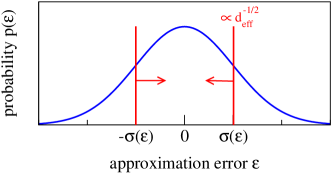
The main point of Eq. (13), however, is that, in addition to the mean error , one also knows the standard deviation of errors , as illustrated in Fig. 1. Precisely, one knows an upper bound for bartsch2009 ; elsayed2013 ; steinigeweg2014-1 ,
| (14) |
where , the effective dimension of the Hilbert space, occurs. In the high-temperature limit , is identical to the full dimension . Thus, if the number of sites is increased, decreases exponentially fast with . Therefore, remarkably, the single pure-state contribution from the first term on the r.h.s. of Eq. (13) turns into an exponentially good approximation for the autocorrelation function. At arbitrary , is the partition function and the ground-state energy, i.e., essentially is the number of thermally occupied states. Again, this number scales exponentially fast with steinigeweg2014-1 but less quickly. To summarize, discarding in Eq. (13) is an approximation which is exact in the thermodynamic limit . At finite , errors can be reduced additionally by sampling, however, this sampling turns out to be unnecessary for all examples in this paper.
III.2 Numerical Method
The central advantage of the approximation in Eq. (13) is that it can be calculated without the eigenstates and eigenvalues of the Hamiltonian, in contrast to the exact expression in Eq. (10). Specifically, this calculation is based on the two auxiliary pure states
| (15) | |||
| (16) |
both depending on time and temperature. Note that the only difference between the two states is the additional current operator in the r.h.s. of Eq. (16). By the use of these states, we can rewrite the approximation in Eq. (13) as
| (17) |
where we skip the error for clarity. Apparently, a time dependence of the current operator does not appear anymore in Eq. (17). Instead, the full time and temperature dependence is a property of the pure states only.
The dependence, e.g. of , is generated by an imaginary-time Schrödinger equation,
| (18) |
and the dependence by the usual real-time Schrödinger equation,
| (19) |
These differential equations can be solved by the use of straightforward iterator methods, e.g. Runge-Kutta elsayed2013 ; steinigeweg2014-1 ; steinigeweg2014-2 , or more sophisticated Chebyshev deraedt2007 ; jin2010 schemes. In this paper, we use a fourth order Runge-Kutta (RK4) scheme with a discrete time step . For this small , numerical errors are negligible, as shown later by the time-independent norm of and and the agreement with results from other methods.
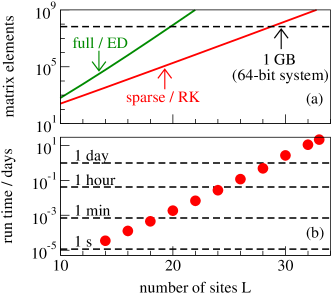
In the Runge-Kutta scheme, we have to implement the action of Hamiltonian and currents on pure states. It is possible to carry out these matrix-vector multiplications without saving matrices in computer memory. Therefore, the memory requirement of the algorithm is set only by the size of vectors: . However, to reduce the run time of the algorithm, it is convenient to save matrices in memory. In this respect, we can profit from the fact that Hamiltonian and currents are few-body operators with a sparse-matrix representation, even in the common eigenbasis of symmetries. In fact, for all operators, there are only nonvanishing matrix elements, as illustrated in Fig. 2 (a). Thus, the memory requirement of the algorithm is and scales linearly with the dimension of the symmetry subspaces. Consequently, we are able to treat chains with as many as sites, where the largest subspaces at are huge:
| (20) |
As compared to the upper subspace dimension accessible to exact diagonalization, this dimension is orders of magnitude larger, i.e., by a factor . Note that the dimension of the full Hilbert space is . In Fig. 2 (b) we show the run time of the algorithm for the largest subspaces and the spin current using a single CPU and discrete time steps (, ). For , the run time is about one month while, for , the calculation takes about two minutes. We note that, for cases where less time steps are needed (, ), calculations are also feasible within reasonable run time, as demonstrated in Sec. IV.1.
Obviously, iterator methods for solving Eqs. (18) and (19) are very typical approaches to profit from massive parallelization. This has been pursued in other applications of typicality, neglecting however the impact of symmetry reduction deraedt2007 . Regarding our algorithm, the latter adds an additional layer of paralellization, i.e., due to the good quantum numbers , each of the subspaces can be computed independently. Remarkably, in practice, we have only relied on the latter paralellization, using not more than CPUs on medium-sized clusters. In this way, we were able to reach system sizes identical to those of massively parallelized codes on super computers without symmetry reduction deraedt2007 ; jin2010 . We believe that symmetry reduction in combination with massive parallelization has the potential to reach in the future.
IV Spin-Current Dynamics in the Integrable Model
First, we present results on the integrable model in Eq. (1). Since the energy current is strictly conserved in this model, we focus on the dynamics of the spin current . Parts of the corresponding results in Figs. 3, 4, and 5 have been shown in our previous work steinigeweg2014-2, . Subsequently, we also investigate the dynamics of the energy current for the nonintegrable model.
IV.1 High Temperatures and Intermediate Times
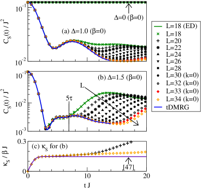
We begin with the high-temperature limit and intermediate times . For anisotropy and small , we compare in Fig. 3 (a) the exact and approximate expressions of the autocorrelation function in Eqs. (10) and (17), numerically calculated by the use of exact diagonalization and fourth order Runge-Kutta, respectively. For all times, the agreement between Eqs. (10) and (17) is remarkably good. Our usage of a semi-log plot underlines this agreement even more and emphasizes relative rather than only absolute accuracy. Due to this agreement, we can already consider the approximation as almost exact for . Moreover, any remaining error decreases exponentially fast with . Thus, we can safely neglect any averaging over random pure states . Note that, for the models studied in this paper, significant errors only occur below , see Appendix D.
By increasing in Fig. 3 (a), we show that the curve of the autocorrelation function gradually converges in time towards the thermodynamic limit. For the maximum size calculated, the curve is converged up to times with no visible finite-size effects in the semi-log plot. For the four largest depicted, we restrict ourselves to a single translation subspace, i.e., , to reduce computational effort in the high-temperature limit . For these temperatures, it is already known that the dependence is negligibly small herbrych2011 , and we also do not observe a significant dependence on for , see Appendix A.
Additionally, we compare to existing tDMRG data for a system of very large size karrasch2012 . It is intriguing to see that our results agree up to very high precession. On the one hand, this very good agreement is a convincing demonstration of dynamical typicality in an integrable system. On the other hand, this agreement unveils that our numerical technique yields exact information on an extended time window in the thermodynamic limit . As shown later, this time window can become very large for nonintegrable systems.
In Fig. 3 (b) we show a second calculation for a larger anisotropy . Clearly, the autocorrelation function decays to almost zero rapidly. However, there is a small long-time tail. This tail has been observed already on the basis of exact diagonalization for intermediate steinigeweg2009 . It is not connected to the Drude weight karrasch2014-1 , as discussed in more detail later. It is also not a finite-size effect, as evident from the agreement with tDMRG. While this tails shows the tendency to decay when comparing and , we relate its origin to the onset of revivals in the vicinity of the Ising limit karrasch2014-1 . If we partially neglect the tail and determine the dc conductivity according to Eq. (11) for , we get . This value agrees well with the theoretically predicted value of the perturbation theory in Ref. steinigeweg2011-1, , see Fig. 3 (c). Because this theory does not take into account the tail, both values slightly differ. For the maximum time without finite-size effects, , we get . This value is still not larger than of theoretical prediction, see also Ref. karrasch2014-1, .
IV.2 Long-Time Limit
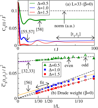
Next, we investigate the long-time limit. In Fig. 4 (a) we show in the high-temperature limit and various anisotropies , , and . Additionally, we depict the norm of . This norm is practically constant, as the norm of also. The constant norm clearly demonstrates that the Runge-Kutta scheme works properly at such long times. The data in Fig. 4 (a) also proves the saturation of at rather long time scales . Furthermore, we can hardly infer the saturation value from our short-time data in Fig. 3. We note that no fluctuations are visible in the long-time limit since the approximation error of our numerical approach is exponentially small and practically zero for the large system sizes depicted.
In contrast to short times, the long-time limit is still governed by finite-size effects. Hence, we are now going to perform a proper finite-size scaling for the Drude weight. We use the definition of the Drude weight according to Eq. (11) and average over the time interval , without invoking assumptions. The Drude weight has been extracted the same way in Ref. steinigeweg2009, . Moreover, this way of extracting the Drude weight reproduces the correct zero-frequency values for small in, e.g., Ref. heidrichmeisner2003, .
In Fig. 4 (b) we depict the resulting Drude weight vs. the inverse length for anisotropies , , and . For , we extract the Drude weight from the approximation in Eq. (17) (denoted by crosses) and, for , we use the exact expression in Eq. (10) (denoted by other symbols). In this way, we avoid typicality errors at small . We also indicate the results of fits, solely based on data points for . In this way, we avoid the need of corrections as well as the influence of even-odd effects at small and, especially, at small evenodd , see Fig. 4 (b). For the small , the resulting fit is close to all data points. Furthermore, extracting the thermodynamic limit from the fit, we find a non-zero Drude weight in convincing agreement with the rigorous lower bound of Refs. prosen2011, ; prosen2013, . While the situation is rather similar for the large anisotropy , the Drude weight vanishes, in agreement with previous work heidrichmeisner2003 . The isotropic point is certainly the most interesting case. Here, the fit is not close to the one obtained from only small . In fact, the extrapolation yields much smaller values for the Drude weight than the finite values suggested in previous works, based on either smaller heidrichmeisner2003 ; karrasch2013-1 or shorter karrasch2012 (see also Ref. karrasch2013-1, for a comprehensive discussion). Moreover, our result points to a vanishing Drude weight for .
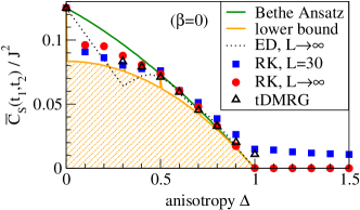
In Fig. 5 we summarize the finite-size values for the Drude weight for fixed and various anisotropies . Additionally, we indicate the extrapolated values for using fits. Since even-odd effects are stronger closer to the point , we take into account only even sites for the fits. Remarkably, all extrapolated values lie above the rigorous lower bound of Refs. prosen2011, ; prosen2013, , and in the anisotropy range , also agree with the Bethe-Ansatz solution of Ref. zotos1999, . They further agree with an alternative extrapolation on the basis of small herbrych2011 , using a different statistical ensemble and only odd sites. In the vicinity of the point , we still lie above the lower bound but we observe deviations from the Bethe-Ansatz result. These deviations do not indicate the breakdown of typicality and are well-known to occur in numerical studies using finite systems herbrych2011 , due to the very high degeneracy at . As visible in Fig. 5, tDMRG results for also show these deviations and are in very good agreement with our results.
IV.3 Low Temperatures
We now turn to finite temperatures . Clearly, the approximation in Eq. (17) has to break down for , i.e., , due to the reduction of the effective Hilbert space dimension . Recall that essentially counts the number of thermally occupied states. Furthermore, for , also the exact expression in Eq. (10) is governed by large finite-size effects, at least for a finite system of size prelovsek2013 . Thus, for a numerical approach to , reasonable temperatures are . For this range of , the approximation is still justified and averaging over pure states is necessary for only. This temperature, however, depends on the specific model, as discussed later in more detail for the nonintegrable system.
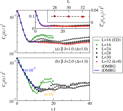
For a small size , anisotropy , and the two lower temperatures and , we compare in Figs. 6 (a) and (b) the exact expression in Eq. (10) and the approximation in Eq. (17), calculated by the use of exact diagonalization and Runge-Kutta, respectively. Clearly, deviations appear at . However, these deviations manifest as random fluctuations rather than systematic drifts and may be compensated by additional averaging over several pure states . Furthermore, one can expect that these deviations disappear for significantly larger sizes . Again, we prove this expectation by comparing with available tDMRG data for karrasch2012 ; karrasch2013-1 . The very good agreement illustrates the power of our numerical approach at finite temperatures. Moreover, taking into account the simple structure of the curve, the semi-log plot, and the combination of tDMRG with our numerical approach, Fig. 6 (a) points to non-zero Drude weights at . This observation is different from our previous results at . Still there are finite-size effects for the three largest values of where a plateau is clearly seen at times . But these finite-size effects are hardly visible in a lin-lin plot, see the inset in Fig. 6 (a). Moreover, extrapolations are impossible on the basis of three and approximately constant points, see the inset therein.
It is further worth mentioning that the possibility of non-vanishing Drude weights at is consistent with the recent upper bound in Ref. carmelo2014, . This upper bound does not vanish when taking into account all sectors of magnetization, as done in our paper.
V Energy-Current Dynamics in the Nonintegrable Model
Next, we extend our analysis in two directions. First, we break the integrability of the model by the staggered magnetic field in Eq. (7). Second, we expand our analysis to include the dynamics of the energy current , which is not conserved anymore in the nonintegrable model.
V.1 Dependence on Magnetic Field and Anisotropy
Again, we begin with the high-temperature limit and compare the exact expression in Eq. (10), evaluated by exact diagonalization, and the approximation in Eq. (17), evaluated by Runge-Kutta, for the energy current . We show this comparison in Figs. 7 (a)-(c) for a small size , anisotropy , and magnetic fields of different strength , , and . Apparently, Eqs. (10) and (17) agree well with each other. This good agreement proofs that dynamical typicality is neither a particular property of the spin current nor restricted to the integrable system. Interestingly, our data already reproduces existing tDMRG data for in Ref. karrasch2013-2, . We note that exact-diagonalization data for does so also, although not shown here explicitly.
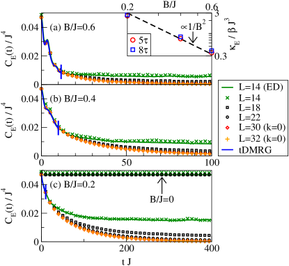
For small and all in Fig. 7 (a)-(c), the energy-current autocorrelation function does not decay to zero and features a nonzero Drude weight. The actual value of the finite-size Drude weight increases as is decreased. However, by increasing , we show that decays to zero for significantly larger and all considered. Moreover, we find that is practically the same for and . This finding indicates little finite-size effects up to full relaxation. Hence, our numerical approach yields exact information on the full, physically relevant time window in the thermodynamic limit .
Let us discuss the relaxation curve for large in more detail. The relaxation time decreases as increases and the overall structure of the curve is simple, in particular without any slowly decaying long-time tails. Therefore, extracting from our numerical data the dc conductivity according to Eq. (11) yields similar values for cutoff times and . These values are shown in the inset of Fig. 7 (a). The apparent decrease of with results from the decrease of with and our usage of a log-log plot unveils the scaling , as expected from conventional perturbation theory at small steinigeweg2010 ; steinigeweg2011-2 . Note that the commutator in Eq. (8) essentially is the memory kernel of the perturbation theory and yields scattering rates and hence, in units of the sum rule, the scaling
| (21) |
i.e., for small values of . A more detailed description of the perturbation theory is given in Appendix B.
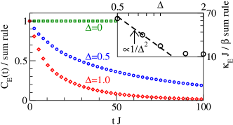
To verify the dependence from perturbation theory, we calculate in Fig. 8 the energy-current autocorrelation function for different , and , at fixed magnetic field and size . Indeed, decays the slower the smaller and no dynamics occurs at . Moreover, extracting the dc conductivity from our numerical data, we find the scaling at small , as shown in the inset of Fig. 8. This scaling turns into at large , still consistent with the expectation from perturbation theory.
V.2 Temperature Dependence
We now turn to finite temperatures and choose the parameters of the model according to the availability of tDMRG data in the literature. Such data is available for negative anisotropy huang2013 , where the model is still antiferromagnetic. We note that the sign of has not been of importance so far since, at high temperatures , the dynamics depends on only.
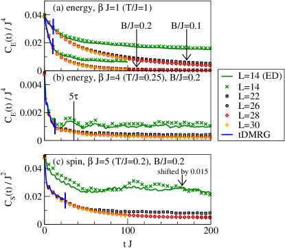
In Figs. 9 (a) and (b) we summarize our results on the energy-current autocorrelation function for an intermediate temperature and a low temperature . Moreover, we depict our results on the spin-current autocorrelation function for an even lower temperature of in Fig. 9 (c). While the focus is on a magnetic field of strength , Fig. 9 (a) also shows results for the case . Several comments are in order. First, already for a small system size of , the exact expression in Eq. (10) and the approximation in Eq. (17) are in good agreement at . While deviations occur at , these deviations are surprisingly small for both, the energy and spin current in Figs. 9 (b) and (c). Second, our exact-diagonalization data for already reproduces existing tDMRG data for in Ref. huang2013, for the whole temperature range . This observation is indeed interesting, especially since lower temperatures have not been analyzed by tDMRG huang2013 , at least for the energy current. Third, our results for large do not depend significantly on . This independence demonstrates the high accuracy of the approximation in Eq. (17) for large and also indicates little (or weakly scaling) finite-size effects.
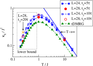
Because we do not need to deal with finite-size effects, we may directly extract from our numerical data the dc conductivity in Eq. (11), starting with the cutoff time . This choice has been sufficient for high temperatures and its role for low temperatures is discussed later in detail. For the energy current and another negative anisotropy , we show in Fig. 10 the resulting temperature dependence of in a log-log plot. Apparently, in the limit of high temperatures . This scaling with is a direct consequence of the trivial prefactor in Eq. (11) and shows that the actual energy-current autocorrelation turns independent in that limit. At , the high-temperature limit is clearly left and features a broad maximum. At , the low-temperature regime sets in and the scaling of with is consistent with a power law, however, the exponent remains an open issue. Remarkably, this power-law scaling mainly results from the initial value and not from the time dependence as such, cf. Figs. 9 (a) and (b).
In Fig. 10 we additionally compare these results on with results from tDMRG. Precisely, we compare to results from fits/extrapolations performed in Ref. huang2013, on the basis of short-time tDMRG data, cf. Figs. 9 (a) and (b). While the overall agreement is quite good, our lies above the one of Ref. huang2013, for all temperatures . We emphasize that this deviation is not a finite-size effect and, moreover, that it does not result from our choice for the calculation of . In fact, using a longer time yields a positive correction to and hence increases the deviation, as illustrated in Fig. 10. This correction is again small at high temperatures: At , the correction is only and, at , the correction is slightly higher with . But the trend indicates that exhibits slowly decaying long-time tails at low temperatures. Furthermore, such a tail is clearly visible at in Fig. 9 (b). For this low temperature, our choice of or seems to underestimate significantly and has to be understood as a lower bound. We explicitly avoid analyzing longer since we cannot exclude the possibility of (weakly scaling) finite-size effects in the long-time limit.
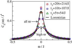
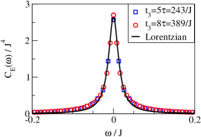
To gain further insight and to provide an alternative point of view, we show in Fig. 11 the Fourier-transformed energy-current autocorrelation function , still for anisotropy and magnetic field , at temperature . This parameter set corresponds to the maximum visible in Fig. 10. The Fourier transform is performed for different , , and . Note that the longest time is . While at does not depend on the specific choice of , it does at . Clearly, a minimum time is required to determine the limit with sufficient accuracy, as a consequence of slowly decaying long-time tails at low temperatures. We also indicate the result of a Lorentzian fit to at . Evidently, this high-frequency/short-time fit cannot be used to predict the dc value correctly. This fact illustrates the origin of the underestimation in Ref. huang2013, . We stress that the overall form of is not Lorentzian at all, while our previous results in the limit of high temperatures agree well with a Lorentzian line shape, see Appendix C.
VI Summary
In summary, we used the concept of typicality to study the real-time relaxation of spin and energy currents in spin- chains at finite temperatures. These chains were the integrable XXZ chain and a nonintegrable version due to the presence of a staggered magnetic field oriented in direction. In the framework of linear response theory, we numerically calculated autocorrelation functions by propagating a single pure state, drawn at random as a typical representative of the full statistical ensemble. By comparing to data from exact diagonalization for small system sizes and existing data from tDMRG for short times, we showed that typicality holds in finite systems over a wide range of temperature and is fulfilled in both, integrable and nonintegrable systems.
For the integrable model, we calculated the dynamics of the spin current for long times and extracted the spin Drude weight for large system sizes outside the range of state-of-the-art exact diagonalization. Employing proper finite-size scaling, we provided strong evidence that, at high temperatures above the exchange coupling constant , the Drude weight vanishes at the isotropic point. This finding, and also our results for other values of the exchange anisotropy, were in good agreement with existing Bethe-Ansatz and Mazur-inequality results. For lower temperatures on the order of , we found at least indications that the Drude weight is nonzero at the isotropic point.
For the nonintegrable model, we calculated the decay of the energy current for large system sizes and did not observe significant finite-size effects. Therefore, we were able to obtain the full decay curve in the thermodynamic limit and to extract the dc conductivity without invoking difficult fits/extrapolations. Analyzing the dependence of the dc conductivity on the parameters of the model, we found a quadratic scaling with the inverse magnetic field and exchange anisotropy, in agreement with conventional perturbation theory. Moreover, we detailed the temperature dependence of the dc conductivity, including low- and high-temperature power laws with an intermediate maximum. Our numerical results seem to provide a lower bound on the dc conductivity.
From a merely numerical point of view, we profit from two central advantages of the typicality-based technique used in this paper. First, the numerical technique allows us to perform finite-size scaling. This is certainly similar to exact diagonalization. However, system sizes are much larger and extrapolations are more reliable. Second, the numerical technique also yields exact information on an extended time window in the thermodynamic limit. This is certainly similar to tDMRG. However, time windows accessible seem to be much longer for generic nonintegrable systems, as evident for the example studied in this paper. Because of these two advantages, our numerical method may complement other numerical approaches in a much broader context, including problems with few symmetries and/or in two dimensions. Moreover, our numerical method may be applied to other observables elsayed2013 and not only to current operators.
Acknowledgments
We sincerely thank H. Niemeyer, P. Prelovšek, and J. Herbrych for fruitful discussions as well as C. Karrasch and F. Heidrich-Meisner for the tDMRG data in Sec. IV (Refs. karrasch2012, ; karrasch2013-1, ; karrasch2014-1, ; karrasch2014-2, ) and helpful comments. The tDMRG data in Sec. V (Refs. karrasch2013-2, ; huang2013, ) have been digitized.
Part of this work has been done at the Platform for Superconductivity and Magnetism, Dresden. Part of this work has been supported by DFG FOR912 Grant No. BR 1084/6-2, by SFB 1143, as well as by EU MC-ITN LOTHERM Grant No. PITN-GA-2009-238475.
Appendix A Independence of the Specific Initial State and Momentum Subspace
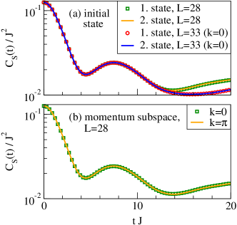
In Fig. 12 we demonstrate that for large system sizes the approximation in Eq. (17) depends neither on the specific realization of the random initial state nor on the momentum subspace considered. Because both facts are particularly relevant for the finite-size scaling of the spin Drude weight in Fig. 4, we present in Fig. 12 results for the integrable model in Eq. (1) at anisotropy in the limit of high temperatures . In this limit, the independence of initial states and momentum subspace holds for all examples given in this paper. For low temperatures, we explicitly avoid the restriction to a single momentum subspace since the independence of is not ensured in this temperature regime, also for the exact expression in Eq. (10).
Appendix B Perturbation Theory for the Energy Current
We discuss here the perturbation theory for the energy current in detail. Since the energy current is strictly conserved for the integrable Hamiltonian , , the staggered Zeeman term can be identified as the only origin of scattering. This scattering can be treated perturbatively according to Refs. jung2006, ; jung2007, ; steinigeweg2010, ; steinigeweg2011-2, if the strength of the magnetic field is a sufficiently small parameter. In the time domain, we can formulate such a perturbation theory in terms of the integro-differential equation
| (22) |
where is the memory kernel. To lowest order of , , this memory kernel reads in the high-temperature limit steinigeweg2010 ; steinigeweg2011-2
| (23) |
where the subscript I of the first commutator indicates the interaction picture w.r.t. . Despite the integrability of , exactly calculating the time dependence of is very difficult and requires, e.g., the exact diagonalization of a finite system jung2006 ; jung2007 . For our purposes, however, it is sufficient to use the well-known Markov approximation . This approximation is reasonable in the limit of small magnetic fields , where relaxation is arbitrarily slow. In this way, we obtain from Eq. (22) the exponential relaxation
| (24) |
corresponding to a Lorentzian line shape in frequency space. Thus, using the expression for the dc conductivity in Eq. (11) with , we find the scaling
| (25) |
The quantity introduced does not include a trivial scaling due to the sum rule and is the prediction of the perturbation theory as such. For small values of , we eventually find the scaling and, for large values of , we find to be independent of . In this case, .
Appendix C Fourier Transform at High Temperatures
In Fig. 13 we show that the Fourier transform of our numerical results for the time-dependent energy-current autocorrelation function at high temperatures, i.e. , yields a Lorentzian line shape of in frequency space. This line shape is another convincing indicator for the validity of conventional perturbation theory.
Appendix D Typicality in Small Systems
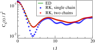
Throughout this paper we have provided a comparison with exact-diagonalization data to prove that typicality already holds in finite systems of intermediate size, i.e., . It is clear that typicality has to break down for small systems. For the models studied in this paper, we observe this breakdown for sizes below , i.e., for effective dimensions below . In Fig. 14 we show one representative example.
However, a simple idea also allows us to use typicality for small : Consider two identical, uncoupled chains of length with the Hamiltonian
| (26) |
and the current , respectively. In this way, we do not change the exact current dynamics but increase the dimension of the Hilbert space by a factor of . For the enlarged space, we can expect that typicality holds again. Figure 14 verifies this expectation.
We emphasize that the preceding is equivalent to averaging. The random state from the dimensional Hilbert space has a Schmidt decomposition
| (27) |
where are random coefficients and , are random orthonormal basis sets for each of the dimensional subspaces. Therefore, using a single random state in the doubled system is equivalent to a randomly weighted average over autocorrelations functions, each calculated using one of randomly chosen states. If this is more efficient than full diagonalization will depend on details.
We note that one can analogously consider more than two chains and therefore use typicality for any smaller .
References
- (1) J. Gemmer and G. Mahler, Eur. Phys. J. B 31, 249 (2003).
- (2) S. Goldstein et al., Phys. Rev. Lett. 96, 050403 (2006).
- (3) S. Popescu, A. J. Short, and A. Winter, Nature Phys. 2, 754 (2006).
- (4) P. Reimann, Phys. Rev. Lett. 99, 160404 (2007).
- (5) S. R. White, Phys. Rev. Lett. 102, 190601 (2009).
- (6) S. Sugiura and A. Shimizu, Phys. Rev. Lett. 108, 240401 (2012).
- (7) C. Bartsch and J. Gemmer, Phys. Rev. Lett. 102, 110403 (2009); EPL 96, 60008 (2011).
- (8) T. A. Elsayed and B. V. Fine, Phys. Rev. Lett. 110, 070404 (2013).
- (9) R. Steinigeweg et al., Phys. Rev. Lett. 112, 130403 (2014).
- (10) R. Steinigeweg, J. Gemmer, and W. Brenig, Phys. Rev. Lett. 112, 120601 (2014).
- (11) A. Hams and H. De Raedt, Phys. Rev. E 62, 4365 (2000).
- (12) J. M. Deutsch, Phys. Rev. A 43, 2046 (1991).
- (13) M. Srednicki, Phys. Rev. E 50, 888 (1994).
- (14) M. Rigol, V. Dunjko, and M. Olshanii, Nature 452, 854 (2008).
- (15) M. A. Cazalilla and M. Rigol, New J. Phys. 12, 055006 (2010); and references therein.
- (16) I. Appelbaum, B. Huang, and D. J. Monsma, Nature 447, 295 (2007).
- (17) N. Tombros et al., Nature 448, 571 (2007).
- (18) N. P. Stern et al., Nature Phys. 4, 843 (2008).
- (19) F. Kuemmeth et al., Nature 452, 448 (2008).
- (20) A. V. Sologubenko et al., Phys. Rev. Lett. 84, 2714 (2000).
- (21) C. Hess et al., Phys. Rev. B 64, 184305 (2001).
- (22) N. Hlubek et al., Phys. Rev. B 81, 20405R (2010).
- (23) K. R. Thurber et al., Phys. Rev. Lett 87, 247202 (2001).
- (24) H. Kühne et al., Phys. Rev. B 80, 045110 (2009).
- (25) H. Maeter et al., J. Phys.: Condens. Matter 25, 365601 (2013).
- (26) F. Xiao et al., arXiv:1406.3202 (2014).
- (27) X. Zotos, F. Naef, and Prelovšek, Phys. Rev. B 55, 11029 (1997).
- (28) A. Klümper and K. Sakai, J. Phys. A 35, 2173 (2002).
- (29) B. S. Shastry and B. Sutherland, Phys. Rev. Lett. 65, 243 (1990).
- (30) X. Zotos, Phys. Rev. Lett. 82, 1764 (1999).
- (31) J. Benz et al., J. Phys. Soc. Jpn. 74, 181 (2005).
- (32) T. Prosen, Phys. Rev. Lett. 106, 217206 (2011).
- (33) T. Prosen and E. Ilievski, Phys. Rev. Lett. 111, 057203 (2013).
- (34) B. N. Narozhny, A. J. Millis, and N. Andrei, Phys. Rev. B 58, 2921R (1998).
- (35) F. Heidrich-Meisner et al., Phys. Rev. B 68, 134436 (2003).
- (36) F. Heidrich-Meisner, A. Honecker, and W. Brenig, Eur. Phys. J. Special Topics 151, 135 (2007).
- (37) J. Herbrych, P. Prelovšek, and X. Zotos, Phys. Rev. B 84, 155125 (2011).
- (38) R. Steinigeweg, J. Herbrych, and P. Prelovšek, Phys. Rev. E 87, 012118 (2013).
- (39) S. Fujimoto and N. Kawakami, Phys. Rev. Lett. 90, 197202 (2003).
- (40) D. C. Johnston et al., Phys. Rev. B 61, 9558 (2000).
- (41) S. Trotzky et al., Science 319, 295 (2007).
- (42) P. Gambardella, Nature Mat. 5, 431 (2006).
- (43) M. Kruczenski, Phys. Rev. Lett. 93, 161602 (2004).
- (44) Y. B. Kim, Phys. Rev. B 53, 16420 (1996).
- (45) K. Fabricius and B. M. McCoy, Phys. Rev. B 57, 8340 (1998).
- (46) R. Steinigeweg and J. Gemmer, Phys. Rev. B 80, 184402 (2009).
- (47) R. Steinigeweg and W. Brenig, Phys. Rev. Lett. 107, 250602 (2011).
- (48) A recent review is given in: P. Prelovšek and J. Bonča, Ground State and Finite Temperature Lanczos Methods in Strongly Correlated Systems, Solid-State Sciences 176 (Springer, Berlin, 2013).
- (49) M. Mierzejewski and P. Prelovšek, Phys. Rev. Lett. 105, 186405 (2010).
- (50) R. Steinigeweg et al., Phys. Rev. B 85, 214409 (2012).
- (51) J. V. Alvarez and C. Gros, Phys. Rev. Lett. 88, 077203 (2002).
- (52) S. Grossjohann and W. Brenig, Phys. Rev. B 81, 012404 (2010).
- (53) S. Langer et al., Phys. Rev. B 79, 214409 (2009).
- (54) S. Jesenko and M. Žnidarič, Phys. Rev. B 84, 174438 (2011).
- (55) C. Karrasch, J. H. Bardarson, and J. E. Moore, Phys. Rev. Lett. 108, 227206 (2012).
- (56) C. Karrasch et al., Phys. Rev. B 87, 245128 (2013).
- (57) C. Karrasch, J. E. Moore, and F. Heidrich-Meisner, Phys. Rev. B 89, 075139 (2014).
- (58) C. Karrasch, D. M. Kennes, J. E. Moore, Phys. Rev. B 90, 155104 (2014).
- (59) Y. Huang, C. Karrasch, and J. E. Moore, Phys. Rev. B 88, 115126 (2013).
- (60) C. Karrasch, R. Ilan, and J. E. Moore, Phys. Rev. B 88, 195129 (2013).
- (61) T. Prosen and M. Žnidarič, J. Stat. Mech.: Theory Exp. 2009, P02035.
- (62) M. Žnidarič, Phys. Rev. Lett. 106, 220601 (2011).
- (63) O. F. de Alcantara Bonfim and G. Reiter, Phys. Rev. Lett. 69, 367 (1992); Phys. Rev. Lett. 70, 249 (1993).
- (64) R. W. Gerling and H. Leschke, Phys. Rev. Lett. 70, 248 (1993).
- (65) R. Steinigeweg, EPL 97, 67001 (2012).
- (66) J. Sirker, R. G. Pereira, and I. Affleck, Phys. Rev. Lett. 103, 216602 (2009); Phys. Rev. B 83, 035115 (2011).
- (67) R. Steinigeweg and R. Schnalle, Phys. Rev. E 82, 040103R (2010).
- (68) R. Steinigeweg, Phys. Rev. E 84, 011136 (2011).
- (69) P. Jung, R. W. Helmes, and A. Rosch, Phys. Rev. Lett. 96, 067202 (2006).
- (70) P. Jung and A. Rosch, Phys. Rev. B 76, 245108 (2007).
- (71) K. De Raedt et al., Comp. Phys. Comm. 176, 121 (2007).
- (72) F. Jin et al., J. Phys. Soc. Jpn. 79, 124005 (2010).
- (73) A. Kolezhuk and H. Mikeska, Lect. Not. Phys. 645, 1 (2004).
- (74) R. Kubo, M. Toda, and N. Hashitsume, Statistical Physics II: Nonequilibrium Statistical Mechanics (Springer, Berlin, 1991).
- (75) J. M. P. Carmelo, T. Prosen, and D. K. Campbell, preprint, arXiv:1407.0732 (2014).
- (76) For , the XXZ Hamiltonian describes a model of free spin-less fermions, , where the single-particle dispersion consists of only points at positions . Thus, for finite , the spectrum of any correlation function in the vicinity of is necessarily sparse and, except for trivial cases, has to feature strong finite-size effects, e.g., even-odd effects.