A Model of Consistent Node Types in Signed Directed Social Networks

Abstract

Signed directed social networks, in which the relationships between users can be either positive (indicating relations such as trust) or negative (indicating relations such as distrust), are increasingly common. Thus the interplay between positive and negative relationships in such networks has become an important research topic. Most recent investigations focus upon edge sign inference using structural balance theory or social status theory. Neither of these two theories, however, can explain an observed edge sign well when the two nodes connected by this edge do not share a common neighbor (e.g., common friend). In this paper we develop a novel approach to handle this situation by applying a new model for node types. Initially, we analyze the local node structure in a fully observed signed directed network, inferring underlying node types. The sign of an edge between two nodes must be consistent with their types; this explains edge signs well even when there are no common neighbors. We show, moreover, that our approach can be extended to incorporate directed triads, when they exist, just as in models based upon structural balance or social status theory. We compute Bayesian node types within empirical studies based upon partially observed Wikipedia, Slashdot, and Epinions networks in which the largest network (Epinions) has 119K nodes and 841K edges. Our approach yields better performance than state-of-the-art approaches for these three signed directed networks.

I Introduction

With the rapid emergence of social networking websites, e.g., Facebook, Twitter, LinkedIn, Epinions, etc., a considerable amount of attention has been devoted to investigating the underlying social mechanisms in order to enhance users’ experiences [17][12][20][13]. Traditional social network analysis concerns itself primarily with unsigned social networks such as Facebook or Myspace which can be modeled as graphs, with nodes representing entities, and positively weighted edges representing the existence of relationships between pairs of entities. Recently, signed directed social networks, in which the relationships between users can be either positive (indicating relations such as trust) or negative (indicating relations such as distrust), are increasingly common. For instance, in Epinions [8], which is a product review website with an active user community, users can indicate whether they trust or distrust other users based upon their reviews; in Slashdot [16][2], which is a technology-related news website, users can tag each other as “friend” or “foe” based upon their comments. Such a signed directed network can be modeled as a graph expressed as an asymmetric adjacency matrix in which an entry is $1$ (or $-1$) if the relationship is positive (or negative) and 0 if the relationship is absent.

One of the fundamental problems in signed social network analysis is edge sign inference [8][18], i.e., inferring the unknown trust or distrust relationship given the existence of a particular edge. To address this issue, many approaches have been developed based upon two main social-psychological theories, i.e., structural balance theory [11][4] and social status theory [19]. Structural balance theory is more well-known and it states that people in signed networks tend to follow the rules that “the friend of my friend is my friend”, “the enemy of my friend is my enemy”, etc. Social status theory, which is implicit in Guha et al. [8], further exploited by Leskovec et al. [19], and based upon a foundation in social psychology [13], considers a positive directed edge to indicate that the initiator of the edge views the recipient as having higher status and a negative directed edge to indicate that the recipient is viewed as having lower status. The relative levels of status determine the allowed sign-direction pairs for an edge assuming that this edge exists.

Although both structural balance theory and social status theory have proved useful for explaining the signs of edges in signed networks, neither is suitable for explaining an observed edge when the two nodes connected by this edge share no common neighbor (e.g., common friend), and in fact, structural balance theory simply does not apply to this situation. Since many real world social networking graphs tend to be very sparse, this is the case for a large fraction of their edges. To better explain the observed edge signs in general, in this paper we develop a novel approach to address this issue by applying a new model for node types.

To summarize the contributions of this paper:

• We explore the underlying local node structures in fully observed signed directed networks, recognizing that there are 16 different types of node and each type of node constrains both its incoming node types and its outgoing node types, i.e., the signs of their edges must be consistent with their types.

• We show that node type features can be extended to incorporate structural balance theory or social status theory, to help make predictions for those edges whose endpoints have common neighbors.

• For the purpose of practical applications, we derive Bayesian node features (including Bayesian node type and Bayesian node properties) based upon partially observed signed directed networks.

• We conduct empirical studies based upon three real world datasets and show that our proposed approach can outperform state-of-the-art algorithms.

II Related Work

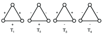
Figure 1: Undirected signed triads. Structural balance theory states that $\text{T}_{1}$ and $\text{T}_{2}$ are balanced, while $\text{T}_{3}$ and $\text{T}_{4}$ are unbalanced. Weak structural balance theory states that $\text{T}_{1}$, $\text{T}_{2}$, and $\text{T}_{4}$ are balanced, while only $\text{T}_{3}$ is unbalanced.

In the past few years, many approaches have been developed to explore different aspects of signed networks, ranging from edge sign prediction [8][18][5][10] to community detection [15][1]. Most of these approaches are based upon structural balance theory or social status theory.

II-A Structural balance theory

The investigation of signed networks [11][4][7][6] can be traced back to the 1920s. Heider [11] first formulated structural balance theory within social psychology. After that, Cartwright and Harary [4] formally provided the notion of structural balance with undirected triads (as shown in Figure 1) and proved its necessity and sufficiency by utilizing the mathematical theory of graphs. Intuitively, their theory can be explained as: “the friend of my friend is my friend” ($\text{T}_{1}$), “the enemy of my friend is my enemy” ($\text{T}_{2}$), “the friend of my enemy is my enemy” ($\text{T}_{2}$), and “the enemy of my enemy is my friend” ($\text{T}_{2}$). Conceptually, their theory claims that $\text{T}_{1}$ and $\text{T}_{2}$ are balanced while $\text{T}_{3}$ and $\text{T}_{4}$ are unbalanced. Davis [6] further generalized this theory to weak structural balance theory by allowing all the edges of triads to be negative, i.e., “the enemy of my enemy is my enemy” ($\text{T}_{4}$ is also balanced). Note that these two balance theories were initially intended for modeling undirected networks, although they have been commonly applied to directed networks by disregarding the direction of edges [19].

II-B Social status theory

Guha et al. [8] first considered the edge sign prediction problem by developing a trust propagation framework to predict the trust (or distrust) between pairs of nodes. In their framework, they calculate a combined matrix which is a linear combination of four different one-step propagations, i.e., direct propagation, co-citation, transpose trust, and trust coupling. Then the trust and distrust propagations are achieved by calculating a linear combination of powers of this combined matrix. A shortcoming of this approach is that it cannot be explained by structural balance theory [4][11].

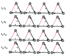
Figure 2: All contexts of ($x$, $y$; $z$). The red edge’s sign is not available; it can be determined based upon $x$’s and $y$’s interactions with $z$. Take $t_{1}$ for example: since $y$ gives $z$ a positive evaluation and $z$ gives $x$ a positive evaluation, $x$ tends to give $y$ a negative evaluation because $x$ has higher status.

Motivated by this trust propagation idea [8] and informed by social psychology [13], Leskovec et al. [19] developed social status theory to explain signed directed networks. In this theory, they assume that if there is a positive edge from $x$ to $y$, it represents the fact that $x$ regards $y$ as having higher status than himself (or herself), and if there is a negative edge from $x$ to $y$, it represents the fact that $x$ regards $y$ as having lower status than himself (or herself). Assuming everyone in the system agrees on the same status ordering, we can infer signs easily as long as the existence and direction of edges are available. When prior status information for $x$ and $y$ is not available, we can still perform sign inference using the context provided by the rest of the network. For instance, in Figure 2, the sign of $x$ to $y$ can be inferred by referring to the status of $z$, and is unambiguous in half the cases.

II-C Approaches to edge sign prediction

Based upon structural balance theory and social status theory, Leskovec et al. [18] selected degree features and directed triad features for edges in signed directed networks. Specifically, for the edge from node $x$ to node $y$, they consider seven degree features, i.e., $d_{\text{in}}^{+}(y)$ and $d_{\text{in}}^{-}(y)$, the number of incoming positive and negative edges to $y$, respectively; $d_{\text{out}}^{+}(x)$ and $d_{\text{out}}^{-}(x)$, the number of outgoing positive and negative edges from $x$, respectively; $C(x,y)$, the number of common neighbors (i.e., embeddedness) of node $x$ and node $y$; $d_{\text{out}}^{+}(x)+d_{\text{out}}^{-}(x)$ and $d_{\text{in}}^{+}(y)+d_{\text{in}}^{-}(y)$, the total out-degree of $x$ and the total in-degree of $y$, respectively. Since each of the 16 triad types in Figure 2 provides different evidence for the sign of the edge from node $x$ to node $y$, directed triad features of this edge are encoded in a 16-dimensional vector counting the number of triads of each type in which this edge is involved. After computing the degree or directed triad features for the edge from $x$ to $y$, a logistic regression classifier is used to combine the evidence from these individual features into an edge sign prediction.

Subsequently, Chiang et al. [5] extended this approach by considering longer cycles (e.g., quadrilaterals, pentagons) while ignoring the directions of edges to reduce the computational complexity. Hsieh et al. [10] formulated the sign inference problem as a low rank matrix completion (approximation) problem based upon weak balance theory. Note that this approach was originally developed to explain a signed undirected network which is associated with a symmetric adjacency matrix and is different from our setting (signed directed networks) in this paper.

We remark that structural balance theory is also popular for community detection in signed networks [15][1].

Although many approaches based upon structural balance theory or social status theory have been developed to perform edge sign prediction in signed networks, they cannot work well when few topological features, i.e., undirected (or directed) triads and long-range cycles, are available in the network. Since many real world signed directed social networking graphs are very sparse, the efficacy of methods based upon these theories is limited. A more general approach for such networks is necessary.

TABLE I: Dataset statistics.

Datasets	Wikipedia	Slashdot	Epinions
Nodes	7,118	82,144	119,217
Edges	103,747	549,202	841,372
$+$edges	78.78$\%$	77.4$\%$	85.0$\%$
$-$edges	21.21$\%$	22.6$\%$	15.0$\%$

III Datasets

In this paper, we consider three well-known signed directed social networks: Wikipedia [3], Slashdot [14][16] and Epinions [8] :

• The Wikipedia data comprise a voting network for promoting candidates to the role of admin. The voters, half coming from existing admins and another half coming from ordinary Wikipedia users, can indicate a positive (for supporting) or negative (for opposing) vote with respect to the promotion of a candidate [18].

• Slashdot is a social website focusing on technology related news. In Slashdot Zoo, users can tag each other as friends (like) or foes (dislike) based upon comments on articles.

• Epinions, which is a product review website, is a trust network in which users can indicate whether they trust or distrust each other based upon their reviews.

The detailed statistics of these datasets are provided in Table I. Note that in all three datasets, the majority of the edges is positive. Due to this imbalance, simply predicting all edges to be positive would yield 78.78$\%$, 77.4$\%$, and 85.0$\%$ accuracy across the three datasets. To show the effectiveness of any approach, it should achieve substantially better performance than this.

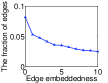
(a) Wikipedia

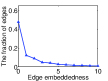
(b) Slashdot

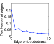
(c) Epinions

Figure 3: The fraction of edges vs. edge embeddedness for three datasets.

Figure 3 shows the fraction of edges versus edge embeddedness [9] (the number of common neighbors of the two nodes connected by the edge) for three datasets. We observe that the edges with zero embeddedness comprise about $8.17\%$, $47.90\%$, $19.88\%$ of the edges for Wikipedia, Slashdot, and Epinions, respectively. Note that a large fraction of zero embeddedness edges means that triad features [18] cannot work well for edge sign prediction. This is because the entries of triad feature vector will be zero and thus the triad features provide no evidence for edge sign prediction.

IV Node Types in Fully Observed Networks

In this paper, a fully observed signed directed network refers to a network in which there is no uncertainty about the existence of any directed edge and its associated sign.

We consider a fully observed signed directed network as a graph $G=(V,E,W)$, where $V$ is the vertex set of size $n$, $E$ is the edge set of size $m$, and $W\in\mathbb{R}^{n\times n}$ is the associated signed adjacency matrix. Because $G$ is a directed network, $W$ is an asymmetric matrix and can be represented as:

$$W_{ij}=\left\{\begin{array}[]{ll}\vspace{0mm}1,&\hbox{if $i$ trusts $j$}\\ -1,&\hbox{if $i$ distrusts $j$}\\ 0,&\hbox{otherwise}\vspace{0mm}\end{array}\right.$$ (4)

Note that $W_{ij}=0$ represents no directed edge from node $i$ to node $j$.

In this section, we first investigate local node structures within fully observed signed directed networks, recognize a set of node types, show that these node types can be used to explain real world signed directed social networks, and show how to encode a specific node in such networks. Next, we explore how these node types interact with one another and how these interactions can explain the edge signs. Finally, we show our approach can be extended to incorporate structural balance theory or social status theory.

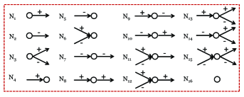
Figure 4: 16 node types in signed directed networks. For $\text{N}_{1}$ (node type 1), all the outgoing edges are positive. For $\text{N}_{5}$, all the incoming edges are negative. For $\text{N}_{15}$, both the incoming edges and outgoing edges are mixtures of positive edges and negative edges.

IV-A Node types

In our study, we focus on analyzing signed directed networks because they are more general and common than signed undirected networks in real world applications. For instance, each of the three datasets we consider in this paper is a signed directed network. Generally, signed directed networks are sparse graphs in which nodes may be categorized into 4 groups based upon whether they have incoming edges and outgoing edges, i.e., nodes with neither incoming nor outgoing edges (e.g., $\text{N}_{16}$ in Figure 4), nodes with only incoming edges (e.g., $\text{N}_{4}$, $\text{N}_{5}$, and $\text{N}_{6}$ in Figure 4), nodes with only outgoing edges (e.g., $\text{N}_{1}$, $\text{N}_{2}$, and $\text{N}_{3}$ in Figure 4), and nodes having both incoming and outgoing edges (e.g., $\text{N}_{9}$, $\text{N}_{14}$, $\text{N}_{15}$, etc.). Moreover, both the incoming edges and the outgoing edges of a given node can be categorized into 3 classes, one class with only positive edges, another class with only negative edges, and the third class with a mixture of positive and negative edges. Combining these two principles, the nodes in signed directed networks can be categorized into 16 types, shown in Figure 4. Note that the edges in Figure 4 only indicate the types of the incoming or outgoing, i.e., they do not represent the actual nonzero number of incoming (outgoing) positive (negative) edges. The fractions of each node type for the three real world datasets are shown in Figure 5.

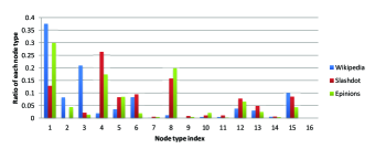
Figure 5: The fractions of different node types for the three datasets.

IV-A1 The representation of node features

To represent each node effectively, in addition to its node type N, we should consider its associated node properties, i.e., the relative level of the number of positive (negative) incoming edges $d_{\rm in}(+)$ $\big{(}d_{\rm in}(-)\big{)}$, and the relative level of the number of positive (negative) outgoing edges $d_{\rm out}(+)$ ($d_{\rm out}(-)$).

First, we can use a 16-dimensional binary vector, $[\textbf{1}(\text{N}=\text{N}_{1})$,$\textbf{1}(\text{N}=\text{N}_{2})$,…, $\textbf{1}(\text{N}=\text{N}_{16})]$, to indicate the node type. The indicator $\textbf{1}(\text{N}=\text{N}_{i})$ is 1 if N is the same as $\text{N}_{i}$. Next, we can use a vector $[\text{P}_{\rm in}(+),\text{P}_{\rm in}(-),$ $\text{P}_{\rm out}(+),\text{P}_{\rm out}(-)]$ to denotes the ratio of positive (negative) incoming edges and that of positive (negative) outgoing edges.

Intuitively, $\text{P}_{\rm in}(+)$, $\text{P}_{\rm in}(-)$, $\text{P}_{\rm out}(+)$, and $\text{P}_{\rm out}(-)$ represent the locally propagating properties of a node (node property) and they can be calculated with

$$\text{P}_{\rm in}(+)=\frac{d_{\rm in}(+)}{d_{\rm in}(+)+d_{\rm in}(-)+\varepsilon}$$ (5)

$$\text{P}_{\rm in}(-)=\frac{d_{\rm in}(-)}{d_{\rm in}(+)+d_{\rm in}(-)+\varepsilon}$$ (6)

$$\text{P}_{\rm out}(+)=\frac{d_{\rm out}(+)}{d_{\rm out}(+)+d_{\rm out}(-)+\varepsilon}$$ (7)

$$\text{P}_{\rm out}(-)=\frac{d_{\rm out}(-)}{d_{\rm out}(+)+d_{\rm out}(-)+\varepsilon},$$ (8)

where we set $\varepsilon=10^{-10}$ to avoid zero denominators. Figure 6 shows examples of these two parts of features for node type $\text{N}_{3}$, $\text{N}_{11}$, and $\text{N}_{15}$. Notice that $\text{P}_{\rm in}(+)+\text{P}_{\rm in}(-)=1$ if there is any input edge, but this sum is zero if there are none; so these features are not redundant. Also note that node property is essentially different from degree features because degree features aim to model a particular edge by considering the initiator’s outgoing edges, recipient’s incoming edges, and their common neighbors.

Note that although the node properties, i.e., $[\text{P}_{\rm in}(+),\text{P}_{\rm in}(-),$$\text{P}_{\rm out}(+),\text{P}_{\rm out}(-)]$ implicitly indicate the node type information, it is still useful to consider type indication, i.e., $[\textbf{1}(\text{N}=\text{N}_{1})$,$\textbf{1}(\text{N}=\text{N}_{2})$,…, $\textbf{1}(\text{N}=\text{N}_{16})]$. Since the latter is not a linear combination of the former, it can provide non-redundant information in the logistic regression classifier we will describe in the Section 6.

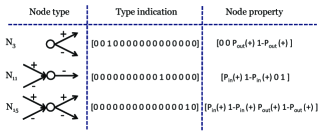
Figure 6: Two parts of the features for node types $\text{N}_{3}$, $\text{N}_{11}$, and $\text{N}_{15}$. Notice that the first (last) two numbers in the second part need not sum to $1$.

IV-B The interaction of node types

We have shown there are 16 possible node types in any signed directed network. Hence, theoretically there are $16^{2}$ combinations of node types. Given a node of a certain type, however, it usually can only connect to (or be reached from) nodes in a subset of these types due to the compatibility of both directions and signs. In other words, there exists a logic to determine whether two nodes can be reached or not and whether the sign should be positive or negative. For instance, given a node of type $\text{N}_{5}$, it can only be connected from a node of type $\text{N}_{2},\text{N}_{3},\text{N}_{7},\text{N}_{9},\text{N}_{11},\text{N}_{13},\text{N}_{14},$ or $\text{N}_{15}$ and the edge sign can only be negative. Similarly, given a node of type $\text{N}_{9}$, it can only be connected from a node of type $\text{N}_{1},\text{N}_{3},\text{N}_{8},\text{N}_{10},\text{N}_{12},\text{N}_{13},\text{N}_{14},$ or $\text{N}_{15}$ and connected to a node of type $\text{N}_{5},\text{N}_{6},\text{N}_{7},\text{N}_{10},\text{N}_{11},\text{N}_{12},\text{N}_{14}$, or $\text{N}_{15}$. Moreover, the edge sign is determined as positive and negative, respectively.

Given an edge from $x$ to $y$, based upon the combinations of node type $x$ and node type $y$, this edge can be categorized into three classes. $``+"$ denotes the edge sign is determined to be positive, $``-"$ denotes the edge sign is determined to be negative, and $``?"$ denotes the edge sign that cannot be determined by the interaction of current two node types, i.e., the edge sign can be either positive or negative. In our three datasets, there are $29945$, $250487$ and $500309$ determined edges (i.e., $``+"$ and $``-"$) for Wikipedia, Slashdot and Epinions, respectively, each a large fraction of the total edges.

Although node types have shown their effectiveness for explaining the edge signs in fully observed signed social networks, there exists a fraction of the total edges for which signs cannot be explained simply by node types. In this case, we can incorporate structural balance or social status theory with node types to address this issue.

IV-C Incorporating structural balance or social status theory

As we described the node types and the interactions of these node types in the previous subsections, we did not need to consider whether there is any common neighbor for a pair of nodes. We should, however, be aware that when common neighbors exist for a pair of nodes, structural balance or social status theory may help to explain the sign of an edge between them.

In Figure 7, for instance, since $\text{N}_{13}$ has both positive and negative outgoing edges and $\text{N}_{15}$ has both positive and negative incoming edges, the sign of the edge between them cannot be determined by the interaction of these two types. Since $\text{N}_{13}$ and $\text{N}_{15}$ have two common neighbors, however, the sign of the edge between them may be explained by either structural balance theory or social status theory. Within structural balance theory, we can disregard the directions of these two triads. From the red (dotted) triad, we can infer the sign of the edge between $\text{N}_{13}$ and $\text{N}_{15}$ to be positive based upon the rule that “my friend’s friend is my friend”. From the blue (dashed) triad, on the contrary, we can infer the sign of this edge to be negative based upon the rule that “my friend’s enemy is my enemy”. Within social status theory, since both the red (dotted) triad and the blue (dashed) triad indicate that $\text{N}_{13}$ has higher status than $\text{N}_{15}$, they consistently imply that the sign of the edge from $\text{N}_{13}$ to $\text{N}_{15}$ is negative.

To incorporate these directed triads as features, we use the same approach as Leskovec et al. [18][19]. Given an edge from $x$ to $y$, and a common neighbor $z$ of $x$ and $y$, the edge between $x$ and $z$ can have four possible configurations, i.e., $x\mathrel{\overset{+}{\longrightarrow}}z$, $x\mathrel{\overset{-}{\longrightarrow}}z$, $x\mathrel{\overset{+}{\longleftarrow}}z$, and $x\mathrel{\overset{-}{\longleftarrow}}z$. Similarly, there are four possible signed edges between $z$ and $y$. Hence we can obtain 16 types of triads each of which may provide different evidence about the sign of the edge from $x$ to $y$.

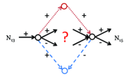
Figure 7: Examples for incorporation of structural balance theory or social status theory into the node types interaction.

V Bayesian Node Features in Partially
Observed Networks

In real world applications, signed directed networks are often partially observed, i.e., several edges’ signs are unknown or hidden. For example, in the Wikipedia dataset, we probably know that someone has voted on a candidate, but we may not know this voter’s opinion. In this case, we would like to infer this voter’s opinion by learning some patterns based upon observed edges in the network. However, when these unobserved edges take different signs, both the node types and node properties may change. In this case, simple node features (including node types and node properties) may not be capable of capturing the range of possible unobserved signs and thus will be not reliable.

To address this issue, we extend node features to Bayesian node features by considering prior knowledge about unobserved signs in partially observed signed directed networks.

Similarly to a fully observed signed directed network, a partially observed signed directed network can also be represented as a graph $G=(V,E,W)$, where $V$ is the vertex set of size $n$, $E$ is the edge set of size $m$, and $W\in\mathbb{R}^{n\times n}$ is the associated signed adjacency matrix. Since $G$ is a directed network, $W$ is an asymmetric matrix and can be represented as:

$$W_{ij}=\left\{\begin{array}[]{ll}\vspace{0mm}1,&\hbox{if $i$ trusts $j$}\\ -1,&\hbox{if $i$ distrusts $j$}\\ $?$,&\hbox{an edge from $i$ to $j$ exists, but sign is unknown}\\ 0,&\hbox{otherwise}\vspace{0mm}\end{array}\right.$$ (13)

$W_{ij}=0$ represents no directed edge from node $i$ to node $j$.

In this section, we first introduce Bayesian node type, show how to calculate it based upon both observed (training) edges and unobserved (test) edges, and present two ways to encode the interaction of Bayesian node types. Next, we show how to calculate and represent Bayesian node properties.

V-A Bayesian node type

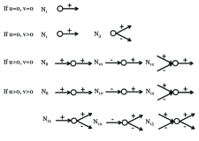
Figure 8: The possible node of type 1 with different $u$ and $v$.

Given any node in a partially observed network, assuming $u$ denotes the number of unobserved incoming edges and $v$ denotes the number of unobserved outgoing edges, let $P_{u}(+)$ (or $P_{u}(-)$) represent the prior probability of incoming edges being positive (negative) and $P_{v}(+)$ (or $P_{v}(-)$) represent the prior probability of outgoing edges being positive (negative). From these probabilities, we can calculate its probability distribution over node types.

Take a node of type $\text{N}_{1}$ for example (as shown in Figure 8), if $u=0$ and $v=0$, its node type does not change; if $u=0$ and $v>0$, it has $(P_{v}(+))^{v}$ probability to be $\text{N}_{1}$ and $1-(P_{v}(+))^{v}$ probability to be $\text{N}_{3}$; if $u>0$ and $v=0$, it has $(P_{u}(+))^{u}$ probability to be $\text{N}_{8}$, $(P_{u}(-))^{u}$ probability to be $\text{N}_{10}$, and $1-(P_{u}(+))^{u}-(P_{u}(-))^{u}$ probability to be $\text{N}_{12}$; if $u>0$ and $v>0$, it has $(P_{u}(+))^{u}(P_{v}(+))^{v}$ probability to be $\text{N}_{8}$, $(P_{u}(-))^{u}(P_{v}(+))^{v}$ probability to be $\text{N}_{10}$, $(1-(P_{u}(+))^{u}-(P_{u}(-))^{u})(P_{v}(+))^{v}$ probability to be $\text{N}_{12}$, $(P_{u}(+))^{u}(1-(P_{v}(+)^{v}))$ probability to be $\text{N}_{13}$, $(P_{u}(-))^{u}(1-(P_{v}(+)^{v}))$ probability to be $\text{N}_{14}$, and $(1-(P_{u}(+))^{u}-(P_{u}(-))^{u})$ $(1-(P_{v}(+)^{v}))$ probability to be $\text{N}_{15}$. This calculation determines a 16 dimensional vector which encodes the distribution of possible node types. Note that similar vectors can be calculated for other types of nodes. We do not specify the calculation for each node type due to the the space limit.

To initialize $P_{u}(+)$ and $P_{v}(+)$, we can also use the Bayesian node properties $P_{\text{in}}(+)$ and $P_{\text{out}}(+)$, i.e., $P_{u}(+)=P_{\text{in}}(+)$ and $P_{v}(+)=P_{\text{out}}(+)$, to claim that each unobserved edge obeys Bayesian node properties (i.e., local priors).

Given an observed (training) edge connecting node $x$ and node $y$, we can obtain two vectors $V_{x}\in\mathbb{R}^{16}$ and $V_{y}\in\mathbb{R}^{16}$ by calculating their Bayesian node types. To encode the interaction of Bayesian node types, we can (1) simply concatenate these two vectors to form a 32 dimensional vector; or (2) calculate the Kronecker product of these two vectors, i.e., $V_{x}\bigotimes V_{y}$, and form a 256 dimensional vector. We should be aware that the vector formed by the Kronecker product encodes the probability distribution of different node type interactions.

Given an unobserved (test) edge connecting node $x$ and node $y$, we should consider both possible signs as shown in Figure 9. Specifically, we first decompose this kind of interaction into two separate cases, i.e., the edge sign being positive and negative. Next, we calculate the Bayesian node types, represent their interactions (either concatenation vector or Kronecker product vector) of both cases. Finally, we calculate the linear combination of these two cases with respect to the prior probability of the signs (i.e., $P(+)$ and $P(-)$) over observed edges.

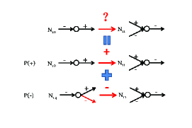
Figure 9: Example of calculating the Bayesian node type interaction when two nodes are connected with an unobserved edge. Note that the Bayesian node types of $\text{N}_{10}$, $\text{N}_{11}$,and $\text{N}_{14}$ should be calculated similar with $\text{N}_{1}$ in Figure 8.

V-B Bayesian node properties

Given a node in a partially observed network, assuming $u$ denotes the number of unobserved incoming edges and $v$ denotes the number of unobserved outgoing edges, by assigning to these $u+v$ edges different signs, the node properties also change.

To capture the range of possible signs of unobserved edges, we should consider Bayesian node properties, i.e., incorporating prior information, namely the expected number of incoming positive (negative) and outgoing positive (negative) edges, with the number of positive (negative) incoming edges $d_{\rm in}(+)$ $\big{(}d_{\rm in}(-)\big{)}$ or outgoing edges $d_{\rm out}(+)$ $\big{(}d_{\rm out}(-)\big{)}$.

Specifically, the Bayesian node properties are represented as following:

$$\text{P}_{\rm in}(+)=\frac{d_{\rm in}(+)+P(+)u}{d_{\rm in}(+)+d_{\rm in}(-)+u+\varepsilon}$$ (14)

$$\text{P}_{\rm in}(-)=\frac{d_{\rm in}(-)+P(-)u}{d_{\rm in}(+)+d_{\rm in}(-)+u+\varepsilon}$$ (15)

$$\text{P}_{\rm out}(+)=\frac{d_{\rm out}(+)+P(+)v}{d_{\rm out}(+)+d_{\rm out}(-)+v+\varepsilon}$$ (16)

$$\text{P}_{\rm out}(-)=\frac{d_{\rm out}(-)+P(-)v}{d_{\rm out}(+)+d_{\rm out}(-)+v+\varepsilon},$$ (17)

where $P(+)$ is the prior probability of positive edges and $P(-)$ is the prior probability of negative edges.

To encode the interaction of Bayesian node properties, we simply concatenate two of the Bayesian node properties vectors to form an 8 dimensional vector.

As in the previous section, when common neighbors exist for a pair of nodes, structural balance or social status theory may be incorporated with Bayesian node features to help explain the sign of an edge between them.

VI Supervised Learning of the
Proposed Features

Given a fully observed signed directed network, the node type interactions, extended to triads with structural balance or social status theory, are useful to explain the edge signs. Partially observed signed directed networks, however, are too complicated to fully conform to the rules of simple node type interactions. Also, as illustrated in Figure 7, if there are multiple common neighbors for $\text{N}_{13}$ and $\text{N}_{15}$, structural balance theory (or social status theory) may conflict with itself. To address this issue, we can utilize a logistic regression to combine the evidence from the interaction of Bayesian node features and triad features.

We now consider the features collected for the logistic regression. The features we utilize can be divided into three classes. One class comes from Bayesian node type interaction (32 or 256 dimensional vector); another class is based upon Bayesian node properties interaction (8 dimensional vector); the last class is triads (16 dimensional vector).

Given a partially observed signed directed social network, we first use a logistic regression to fit the features of observed edges (training data) and then utilize the learned coefficients to linearly combine the evidence from each individual feature of unobserved edges (test data) so as to predict the sign. The logistic regression can be written in the following form

$$P(\ell=1|\textbf{f})=\frac{1}{1+\exp[-(\textbf{w}^{\rm{T}}\textbf{f}+w_{0})]}$$ (18)

where $\ell\in\{0,1\}$ is the label, $1$ represents positive edge while $0$ represents negative edge. $\textbf{f}\in\mathbb{R}^{d}$ is the feature vector, and $[\textbf{w};w_{0}]\in\mathbb{R}^{d+1}$ are the coefficients we estimate from the features of observed edges (training data).

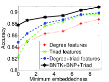
(a) Wikipedia

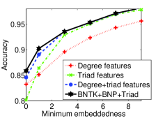
(b) Slashdot

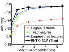
(c) Epinions

Figure 10: The edge sign prediction accuracies of different approaches vs. minimum embeddedness.

VII Experiment

In this section, we conduct empirical studies based upon Wikipedia [3], Slashdot [14][16] and Epinions [8]. We first construct three fully observed asymmetric adjacency matrices (as in Eq.(1)) based upon these three datasets. Next, for each adjacency matrix, we randomly remove 10$\%$ of edges’ signs and form a partially observed network (as in Eq. (6)). Subsequently, we calculate Bayesian node features (including Bayesian node types and Bayesian node properties) and triad features for both observed (training) and unobserved (test) edges. Then, we estimate the parameters of logistic regression based upon the features of observed edges and make predictions based upon the features of unobserved edges. In our experiment, we repeat this procedure 5 times and report the average prediction accuracy and standard deviation for each approach. The baseline approaches are implemented with identical parameter settings as in the original works for fair comparisons.

TABLE II: Step by step justification results on Wikipedia, Slashdot, and Epinions (accuracy: $\%$ and standard deviation (std): $\%$).

	Wikipedia	Slashdot	Epinions
BNTC	83.55($\pm$0.56)	80.32($\pm$0.15)	89.65($\pm$0.04)
BNTK	83.84($\pm$0.12)	80.89($\pm$0.08)	88.34($\pm$0.29)
BNTC+BNP	87.03($\pm$0.15)	84.48($\pm$0.06)	92.96($\pm$0.03)
BNTK+BNP	86.98($\pm$0.19)	84.90($\pm$0.09)	92.46($\pm$0.03)
BNTC+BNP+Triad	87.28($\pm$0.26)	85.24($\pm$0.11)	93.61($\pm$0.02)
BNTK+BNP+Triad	87.37($\pm$0.22)	85.65($\pm$0.11)	93.13($\pm$0.04)

VII-A Step by step justification

We examine the effectiveness of the proposed features by testing each component step by step. We use BNTC to represent encoding the interaction of Bayesian node types with concatenation, use BNTK to represent encoding the interaction of Bayesian node types with the Kronecker product, use BNP to represent the interaction of Bayesian node properties, and use Triad to denote triad features [18][19].

Table II shows the results of step by step justification for edge sign prediction on three datasets. We observe that the interaction of Bayesian node types (BNTC and BNTK) generally outperforms simply predicting all edges to be positive. This demonstrates that the interaction of Bayesian node types is useful to explain the edge signs in partially observed social networks. We also observe that encoding Bayesian node types with the Kronecker product achieves better performance than concatenation on Wikipedia and Slashdot, while concatenation perform slightly better on Epinions.

By concatenating BNTC and BNTK with Bayesian node properties (BNP) features, we observe that BNTC+BNP and BNTK+BNP consistently outperforms BNTC and BNTK. This is because Bayesian node properties (BNP) provide more specific information about the incoming positive (negative) and outgoing positive (negative) edges of nodes.

Finally, we show that, by concatenating BNTC+BNP and BNTK+BNP with triad features to form BNTC+BNP+Triad and BNTK+BNP+Triad, the performances are consistently slightly improved. This is because triad features are useful to explain the edge signs when common neighbors are available.

The step by step justification not only examines the effectiveness of each component of the proposed Bayesian node features, but also shows that the Bayesian node features can incorporate structural balance or social status theory in the form of triad features.

VII-B Edge sign prediction

In this subsection, we compare Bayesian node features (including Bayesian node types and Bayesian node properties) plus triad features with state-of-the-art approaches, i.e., degree features [18], triad features [18], degree$+$triad features [18], longer cycles features [5], and low rank modeling [10]. Note that in our experiment we extract longer cycles features based upon the partially observed asymmetric adjacency matrix and report the best performance over order 3, 4, and 5 for comparison. Also notice that low rank modeling [10] can only theoretically analyze the undirected signed networks; in our experiment, we adapt it and apply it to partially observed signed directed networks.

TABLE III: Edge sign prediction accuracies (accuracy: $\%$ standard deviation (std): $\%$).

Datasets	Wikipedia	Slashdot	Epinions
Degree features [18]	83.58($\pm$0.60)	83.76($\pm$0.13)	90.39($\pm$0.25)
Triad features [19]	82.46($\pm$0.52)	80.42($\pm$0.21)	90.42($\pm$0.13)
Degree+triad features [18, 19]	84.87($\pm$0.08)	84.91($\pm$0.02)	92.25($\pm$0.15)
Longer cycles features [5]	84.04($\pm$0.39)	83.83($\pm$0.34)	90.64($\pm$0.28)
Low rank modeling [10]	84.93($\pm$0.54)	84.57($\pm$0.46)	92.48($\pm$0.32)
BNTC+BNP+Triad	87.28($\pm$0.26)	85.24($\pm$0.11)	93.61($\pm$0.02)
BNTK+BNP+Triad	87.37($\pm$0.22)	85.65($\pm$0.11)	93.13($\pm$0.04)

In Table III, we compare BNTC+BNP+Triad and BNTK+BNP+Triad with the other five state-of-the-art approaches. We observe that BNTC+BNP+Triad and BNTK+BNP+Triad consistently outperform the other five algorithms. Note that these two variants achieve best accuracies of $87.37(\pm 0.22)\%$, $85.65(\pm 0.11)\%$, and $93.61(\pm 0.02)\%$ over Wikipedia, Slashdot and Epinions, respectively. This is because these two variants not only can explain the edge signs well when common neighbors are not available but also can effectively explain the edge signs when common neighbors exist.

In Figure 10, we compare BNTK+BNP+Triad with degree features, triad features, and degree$+$triad features at different levels of embeddedness (the number of common neighbors). In general, we observe that when the minimum embeddedness increases, the performance of BNTK+BNP+Triad increases. This is because structural balance theory and social status theory are incorporated into BNTK+BNP+Triad in the form of triads (Triad) and are effective in explaining edge signs when common neighbors exist. Moreover, we notice that BNTK+BNP+Triad generally outperforms other methods with different levels of embeddedness. This is because BNTK+BNP+Triad leverages the power of node type interactions as well as the power of structural balance or social status theory in the form of triad features (Triad).

VII-C Cross-dataset evaluation

We conduct cross-dataset evaluation with degree features, triad features, degree$+$triad features, and Bayesian node features plus triad features in the form of BNTK$+$BNP$+$Triad on these three datasets. The aim is to examine the generalization capability of each approach. In particular, given each type of features, we train them on one dataset (e.g., Wikipedia) and evaluate the edge sign prediction performance on another (e.g., Slashdot). For each pair of datasets, the test is conducted 5 times based upon the random selected test sets. We report the average accuracies of different approaches in Table IV.

We observe that Bayesian node features plus triad features in the form of BNTK$+$BNP$+$Triad can achieve the best performance on each pair of the cross-dataset evaluation. This illustrates that Bayesian node features plus triad features not only are useful on intra-dataset evaluation but also have good generalization capability. This is extremely helpful for edge sign prediction in signed networks with few training examples.

VIII Conclusions

In this paper, we explored the underlying local node structures in signed networks, recognizing that there are 16 different types of node and each type of node constrains both its incoming node types and its outgoing node types, i.e., the sign of an edge between two nodes must be consistent with their types. This is a highly structured alternative to the ordered scalar node types postulated by social status theory. We demonstrated that the interaction between these more complicated node types can explain edge signs well. We also showed that our approach can be extended to incorporate triad features whose inclusion is motivated by structural balance theory or social status theory. We derived Bayesian node features (including Bayesian node type and Bayesian node properties) based upon partially observed signed directed network. Empirical studies based upon three large scale datasets, i.e., Wikipedia, Slashdot, and Epinions showed that the proposed Bayesian node features plus triad features outperform state-of-the-art algorithms on edge sign prediction. Moreover, we showed that Bayesian node features plus triad features are more effective than baseline approaches for cross-dataset edge sign predictions.

In the future, it will be interesting to study the link recommendation problem based upon Bayesian node features as well as other explicit topological features of signed social networks.

References

- [1] P. Anchuri and M. Magdon-Ismail, Communities and balance in signed networks: A spectral approach, Proceedings of the 4th IEEE/ACM ASONAM, August, 2012.
- [2] M. J. Brozzowski, T. Hogg, and G. Szabo, Friends and foes: ideological social networking, Proceedings of the ACM SIGCHI, pp.817-820, Florence, Italy, 2008.
- [3] M. Burke and R. Kraul, Mopping up: Modeling wikipedia promotion decisions, Proceedings of the ACM Conference on Computer Supported Cooperative Work, pp.27-36, 2008.
- [4] D. Cartwright and F. Harary, Structural balance: A generalization of Heider’s theory, Psych. Rev., vol. 63, no. 5, pp. 277-293, 1956.
- [5] K. Y. Chiang, N. Natarajan, A. Tewari, and I. S. Dhillon, Exploiting longer cycles for link prediction in signed network, Proceedings of the 20th ACM CIKM, pp.1,157-1,162, Glasgow, Scotland, 2011.
- [6] J. A. Davis, Clustering and structural balance in graphs, Human Relations, vol. 20, no. 2, pp. 181-187, 1967.
- [7] O. Frank and F. Harary, Balance in stochastic signed graphs, Social Networks, vol. 2, pp. 155-163, 1979.
- [8] R. V. Guha, R. Kumar, P. Raghavan, and A. Tomkins, Propogation of trust and distrust, Proceedings of the 13th WWW, pp.403-412, New York, NY, 2004.
- [9] M. Granovetter, Economic action and social structure: The problem of embeddedness, American Journal of Sociology, vol. 91, no. 3, pp. 481-510, November, 1985.
- [10] C. J. Hsieh, K. Y. Chiang, and I. S. Dhillon, Low rank modeling of signed network, Proceedings of the ACM SIGKDD, 2012.
- [11] F. Heider, Attitudes and cognitive organization, Journal of Psychology, vol. 21, pp. 107-112, 1946.
- [12] J. Jiang, C. Wilson, X. Wang, P. Huang, Y. Dai, and B. Y. Zhao, Understanding latent interactions in online social networks, Proceedings of the ACM the Internet Measurement Conference, November, 2010.
- [13] C. Kadushin, Understanding social networks: Theories, concepts, and findings, Oxford University Press, 2012.
- [14] J. Kunegis, A. Lommatzsch, and C. Bauckhage, The slashdot zoo: Mining a social network with negative edges, Proceedings of the 19th WWW, pp.541-550, 2009.
- [15] J. Kunegis, S. Schmidt, A. Lommatzsch, J. Lerner, E. W. DeLuca, and S. Albayrak, Spectral analysis of signed graphs for clustering, prediction and visualization, Proceedings of the SIAM SDM, pp.559-570, 2010.
- [16] C. Lampe, E. Johnston, and R. Resnick, Follow the reader: filtering comments on slashdot, Proceedings of the ACM SIGCHI, pp.1,253-1,262, San Jose, CA, 2007.
- [17] D. Liben-Nowell and J. Kleinberg, The link prediction for social networks, Journal of American Society for Information Science and Technology, vol. 58, no. 7, pp. 1,019-1,031, 2007.
- [18] J. Leskovec, D. P. Huttenlocher, and J. M. Kleinberg, Predicting positive and negative links in online social networks, Proceedings of the 20th WWW, pp.641-650, 2010.
- [19] J. Leskovec, D. P. Huttenlocher, and J. M. Kleinberg, Signed networks in social media, Proceedings of the ACM SIGCHI, pp.1,361-1,370, 2010.
- [20] J. Leskovec, K. J. Lang, and M. W. Mahoney, Empirical comparison of algorithms for network community detection, Proceedings of the 20th WWW, 2010.
- [21] S. H. Yang, B. Long, A. Smola, N. Sadagopan, Z. Zheng, and H. Zha, Like like alike - Joint friendship and interest propagation in social networks, Proceedings of the 21st WWW, pp.537-546, 2011.
- [22] X. Yang, H. Steck, and Y. Liu, Circle-based recommendation in online social networks, Proceedings of the ACM SIGKDD, 2012.