A Multi-Plane Block-Coordinate Frank-Wolfe Algorithm
for Training Structural SVMs with a Costly max-Oracle

Abstract

Structural support vector machines (SSVMs) are amongst the best performing models for structured computer vision tasks, such as semantic image segmentation or human pose estimation. Training SSVMs, however, is computationally costly, because it requires repeated calls to a structured prediction subroutine (called max-oracle), which has to solve an optimization problem itself, e.g. a graph cut.

In this work, we introduce a new algorithm for SSVM training that is more efficient than earlier techniques when the max-oracle is computationally expensive, as it is frequently the case in computer vision tasks. The main idea is to (i) combine the recent stochastic Block-Coordinate Frank-Wolfe algorithm with efficient hyperplane caching, and (ii) use an automatic selection rule for deciding whether to call the exact max-oracle or to rely on an approximate one based on the cached hyperplanes.

We show experimentally that this strategy leads to faster convergence to the optimum with respect to the number of requires oracle calls, and that this translates into faster convergence with respect to the total runtime when the max-oracle is slow compared to the other steps of the algorithm.

A publicly available C++ implementation is provided.

1 Introduction

Many computer vision problems have a natural formulation as structured prediction tasks: given an input image the goal is to predict a structured output object, for example a segmentation mask or a human pose. Structural support vector machines (SSVMs) [24, 26], are currently one of the most popular methods for learning models that can perform this task from training data. In contrast to ordinary support vector machines (SVMs) [8], which only predict single values, e.g. a class label, SSVMs are designed such that, in principle, they can predict arbitrary structured objects. However, this flexibility comes at a cost: training an SSVM requires solving a more difficult optimization problem than training an ordinary SVM. In particular, SSVM training requires repeated runs of the structured prediction step (the so called max-oracle) across the training set. Each of these steps is an optimization problem itself, e.g. finding the minimum energy labeling of a graph, and often computationally costly. In fact, the more challenging the problem is, the more the max-oracle calls become a computational bottleneck. This is also a major factor why SSVMs are typically only used for problems with small and medium-sized training sets, not for large scale training as it is common these days, for example, in object categorization [9].

In this work, we introduce a new variant of the Frank-Wolfe algorithm that is specifically designed for training SSVMs in situations where the calls to the max-oracle are the computational bottleneck. It extends the recently proposed block-coordinate Frank-Wolfe (BCFW) algorithm [18] by introducing a caching mechanism that keeps the results of earlier oracle calls in memory. In each step of the optimization, the algorithm decides whether to call the exact max-oracle, or to reuse one of the results from the cache. The first option might allow the algorithm to make a larger steps towards the optimum, but it is slow. The second option will make smaller steps, but this might be justified, since every step will be much faster. Overall, a trade-off between both options will be optimal, and a second contribution of the manuscript is a geometrically motivated criterion for dynamically deciding at any time during the runtime of the algorithm, which choice is more promising.

We report on experiments on four different datasets that reflect a range of structured prediction scenarios: multiclass classification, sequence labeling, figure-ground segmentation and semantic image segmentation.

2 Structural Support Vector Machines

The task of structured prediction is to predict structured objects, $y\in\mathcal{Y}$, for given inputs, $x\in\mathcal{X}$. Structural support vector machines (SSVMs) [24, 26] offer a principled way for learning a structured prediction function, $h:\mathcal{X}\to\mathcal{Y}$, from training data in a maximum margin framework. We parameterize $h(x)=\operatorname*{arg\,max}_{y\in\mathcal{Y}}\langle w,\phi(x,y)\rangle$, where $\phi:\mathcal{X}\times\mathcal{Y}\rightarrow\mathbb{R}^{d}$ is a joint feature function of inputs and outputs, and $\langle\cdot,\,\cdot\rangle$ denotes the inner product in $\mathbb{R}^{d}$. The weight vector, $w$, that is learned from a training set, $\{(x_{1},y_{1}),\dots,(x_{n},y_{n})\}$, by solving the following convex optimization problem:

$$\min_{w} \quad\frac{\lambda}{2}\|w\|^{2}+\sum_{i=1}^{n}H_{i}(w),$$ (1)

where $\lambda\geq 0$ is a regularization parameter. $H_{i}(w)$ is the (scaled) structured hinge loss that is defined as

$$H_{i}(w) \!=\!\frac{1}{n}\!\max_{y\in\mathcal{Y}}\!\big{\{}\Delta(y_{i},y)\!-\!\langle w,\phi(x_{i},y_{i})\!-\!\phi(x_{i},y)\rangle\big{\}},\!\!$$ (2)

where $\Delta:\mathcal{Y}\times\mathcal{Y}\to\mathbb{R}$ is a task-specific loss function, for example the Hamming loss for image segmentation tasks.

Computing the value of $H_{i}(w)$, or the label that realizes this value, requires solving an optimization problem over the label set. We refer to the procedure to do so as the max-oracle, or just oracle. Other names for this in the literature are loss-augmented inference, or just the $\operatorname*{arg\,max}$ step. It depends on the problem at hand how the max-oracle is implemented. We give details of three choices and their properties in Appendix A.

Structural SVMs have proved useful for numerous complex computer vision tasks, including human pose estimation [15, 28], semantic image segmentation [3, 20, 23], scene reconstruction [13, 22] and tracking [14, 19]. In this work, we concentrate not on the question if SSVMs learn better predictors than other methods, but we study Equation (1) from the point of a challenging optimization problem. We are interested in the question how fast for given data and parameters we can find the optimal, or a close-to-optimal, solution vector $w$. This is a question of high practical relevance, since training structured SVMs is known to be computationally costly, especially in a computer vision context where the output set, $\mathcal{Y}$, is large and the max-oracle requires solving a combinatoric optimization problem [20].

2.1 Related Work

Many algorithms have been proposed to solve the optimization problem (1) or equivalent formulations. In [26] and [24], where the problem was originally introduced, the authors derive a quadratic program (QP) that is equivalent to (1) but resembles the SVM optimization problem with slack variables and a large number of linear constraints.

The QP can be solved by a cutting-plane algorithm that alternates between calling the max-oracle once for each training example and solving a QP with a subset of constraints (cutting planes) obtained from the oracle. The algorithm was proved to reach a solution $\epsilon$-close to the optimal one within $O(\frac{1}{\epsilon^{2}})$ step, i.e. $O(\frac{n}{\epsilon^{2}})$ calls to the max-oracle. Joachims et al. improved this bound in [16] by introducing the one-slack formulation. It is also based on finding cutting planes, but keeps their number much smaller, achieving an improved convergence rate of $O(\frac{n}{\epsilon})$. The same convergence rate can also be achieved using bundle methods [25].

Ratliff et al. observed in  [21] that one can also apply the subgradient method directly to the objective (1), which also allows for stochastic and online training. A drawback of this is that the speed of convergence depends crucially on the choice of a learning rate, which makes subgradient-based SSVM training often less appealing for practical tasks.

The Frank-Wolfe algorithm (FW) [10] is an elegant alternative: it resembles subgradient methods in the simplicity of its updates, but does not require a manual selection of the step size. Recently, Lacoste-Julien et al. introduced a block-coordinate variant of the Frank-Wolfe algorithm (BCFW) [18]. It achieves higher efficiency than the original FW algorithm by exploiting the fact that the SSVM objective can be decomposed additively into $n$ terms, each of which is structured. In their experiments, the authors showed a significant speedup of the BCFW algorithm compared to the original FW algorithm as well as the previously proposed techniques.

BCFW can be considered the current state-of-the-art for SSVM training. However, in the next section we show that it can be significantly improved upon for computer vision tasks, in which the training time is dominated by calls to the max-oracle.

3 Efficient SSVM Training

In this section we introduce our main contribution, the multi-plane block-coordinate Frank-Wolfe (MP-BCFW) algorithm for SSVM training. Because it builds on top of the FW and BCFW methods, we start by giving a more detailed explanation of the working mechanisms of these two algorithms. Afterwards, we highlight the improvements we make to tackle the situation when the max-oracle is computationally very costly.

First, we rewrite the structured Hinge loss term (2) more compactly as

$$H_{i}(w)=\max_{y\in{\cal Y}}\;\langle\varphi^{iy},[w\;1]\rangle,$$ (3)

where $\langle\,\cdot,\cdot\,\rangle$ denotes the inner product in $\mathbb{R}^{d+1}$, and $[w\;1]$ is the concatenation of $w$ with a single $1$ entry. For a vector $\varphi\in\mathbb{R}^{d+1}$ we denote its first $d$ components as $\varphi_{\star}\in\mathbb{R}^{d}$ and its last component as $\varphi_{\circ}\in\mathbb{R}$. The data vector $\varphi^{iy}$ in (3) for $i=1,\dots,n$ and $y\in\mathcal{Y}$ is given by $\varphi^{iy}_{\star}=\frac{1}{n}(\phi(x_{i},y)-\phi(x_{i},y_{i}))$ and $\varphi^{iy}_{\circ}=\frac{1}{n}\Delta(y^{i},y)$. Note that $\langle\varphi^{iy},[w\;1]\rangle=\langle\varphi^{iy}_{\star},w\rangle+\varphi^{iy}_{\circ}$.

3.1 Frank-Wolfe algorithm

The Frank-Wolfe (FW) algorithm solves the SSVM training problem in its dual form. Writing $H(w)=\sum_{i=1}^{n}H_{i}(w)$ and introducing concatenated vectors $\varphi^{\bar{y}}=\varphi^{(y_{1},\ldots,y_{n})}=\sum_{i=1}^{n}\varphi^{iy_{i}}$, the primal problem becomes

$$\min_{w}\;\frac{\lambda}{2}||w||^{2}\!+\!H(w),\ \ \text{for}\ H(w)=\max_{\bar{y}\in\overline{{\cal Y}}}\;\langle\varphi^{\bar{y}},[w\,1]\rangle,$$ (4)

for $\overline{{\cal Y}}={\cal Y}\times\cdots\times{\cal Y}$. Note that evaluating $H(w)$ for a given $w$ requires $n$ calls to the max-oracle, one for each of the terms $H_{1}(w),\ldots,H_{n}(w)$.

+

Figure 1: Frank-Wolfe algorithm for minimizing $\frac{\lambda}{2}||w||^{2}+H(w)$. The vector $\varphi$ specifies the current linear lower bound on $H$. One iteration involves three steps: (i) Compute the vector $w$ that minimizes $\frac{\lambda}{2}||w||^{2}+\langle\varphi,[w\;1]\rangle$. (ii) Obtain a new linear bound $\hat{\varphi}$ on $H(\cdot)$ by computing a subgradient of $H$ at $w$. (iii) Compute a linear interpolation $\varphi^{\prime}$ between $\varphi$ and $\hat{\varphi}$ that maximizes $\mathcal{F}(\varphi^{\prime})$, and set $\varphi\leftarrow\varphi^{\prime}$.

The FW algorithm maintains a (hyper)plane specified by a vector $\varphi\in\mathbb{R}^{d+1}$ that corresponds to a lower bound on $H(\cdot)$: $\langle\varphi,[w\;1]\rangle\leq H(w)$ for all $w\in\mathbb{R}^{d}$. Such a plane exists, because $H$ is convex. In fact, any $\varphi^{\bar{y}}$ for $\bar{y}\in\overline{{\cal Y}}$ has this property, as well as any convex combination of such planes, $\varphi=\sum_{\bar{y}\in\overline{\cal Y}}\alpha_{\bar{y}}\varphi^{\bar{y}}$ for $\sum_{\bar{y}\in\overline{\cal Y}}\alpha_{\bar{y}}=1$ and $\alpha_{\bar{y}}\geq 0$. We call vectors $\varphi$ of this form feasible.

Any feasible $\varphi=[\varphi_{\star}\;\varphi_{\circ}]$ provides a lower bound on (4), which we can evaluate analytically

$$\mathcal{F}(\varphi)=\min_{w}\Big{\{}\frac{\lambda}{2}||w||^{2}+\langle\varphi,[w\,1]\rangle\,\Big{\}}=-\frac{1}{2\lambda}||\varphi_{\star}||^{2}+\varphi_{\circ}.$$ (5)

Maximizing $\mathcal{F}(\varphi)$ over all feasible vectors $\varphi$ yields the tightest possible bound. This maximization problem is the dual to (4). The Frank-Wolfe algorithm is iterative procedure for maximizing $\mathcal{F}(\varphi)$. It is stated in pseudo code in Algorithm 1, and it is illustrated in Figure 1. Each iteration monotonically increases $\mathcal{F}(\varphi)$ (unless the maximum is reached), and the algorithm converges to an optimal solution with the rate $O(\frac{1}{\epsilon})$ with respect to the number of iterations, i.e. $O(\frac{n}{\epsilon})$ oracle calls [18].

Algorithm 1 Frank-Wolfe algorithm for the dual of (4)

1:  set $\varphi\leftarrow\varphi^{\bar{y}}$ for some $\bar{y}\in\overline{\cal Y}$

2:  repeat

3:    compute $w\leftarrow\operatorname*{arg\,min}_{w}\frac{\lambda}{2}||w||^{2}+\langle\varphi,[w\;1]\rangle$;   the solution is given by $w=-\frac{1}{\lambda}\varphi_{\star}$

4:    call oracle for vector $w$: compute $\hat{\varphi}\leftarrow\operatorname*{arg\,max}\limits_{\varphi^{\bar{y}}:\bar{y}\in\overline{\cal Y}}\langle\varphi^{\bar{y}},[w\;1]\rangle$

5:    compute $\gamma\leftarrow\operatorname*{arg\,max}_{\gamma\in[0,1]}\mathcal{F}((1-\gamma)\varphi+\gamma\hat{\varphi})$ as follows:       set $\gamma\leftarrow\frac{\langle\varphi_{\star}-\hat{\varphi}_{\star},\varphi_{\star}\rangle-\lambda(\varphi_{\circ}-\hat{\varphi}_{\circ})}{||\varphi_{\star}-\hat{\varphi}_{\star}||^{2}}$ and clip $\gamma$ to $[0,1]$   set $\varphi\leftarrow(1-\gamma)\varphi+\gamma\hat{\varphi}$

6:  until some stopping criterion

3.2 Block-coordinate Frank-Wolfe algorithm

The block-coordinate Frank-Wolfe algorithm [18] also solves the dual of problem (1), but it improves over the FW algorithm by making use of the additive structure of the objective (4). Instead of keeping a single plane, $\varphi$, it maintains $n$ planes, $\varphi^{1},\ldots,\varphi^{n}$, such that the $i$-th plane is a lower bound on $H_{i}$: $\langle\varphi^{i},[w\;1]\rangle\leq H_{i}(w)$ for all $w\in\mathbb{R}^{d}$. Each such plane is obtained as a convex combination of the planes that define $H_{i}(\cdot)$, i.e. $\varphi^{i}=\sum_{y\in{\cal Y}}\alpha_{iy}\varphi^{yi}$ where $\sum_{y\in{\cal Y}}\alpha_{iy}=1$ and $\alpha_{iy}\geq 0$.

We now call a vector $(\varphi^{1},\ldots,\varphi^{n})$ feasible if each $\varphi^{i}$ is as above. The sum $\varphi=\sum_{i=1}^{n}\varphi^{i}$ then defines a plane that lower bounds $H(w)=\sum_{i=1}^{n}H_{i}(w)$, i.e. $\langle\varphi,[w\;1]\rangle\leq H(w)$ for all $w\in\mathbb{R}^{d}$. Therefore, $\mathcal{F}(\varphi)$, as defined by (5), is again a lower bound on problem (1), and the goal is again to maximize this bound over all feasible vectors $(\varphi^{1},\ldots,\varphi^{n})$.

BCFW does so by the block-coordinate strategy. It picks an index $i\in[n]=\{1,\ldots,n\}$ and updates the component $\varphi^{i}$ while keeping all other components fixed. During this step the terms $H_{j}(w)$ for $j\neq i$ are approximated by linear functions $\langle\varphi^{j},[w\;1]\rangle$, and the algorithm tries to find a new linear approximation for $H_{i}(\cdot)$ that gives a larger bound $\mathcal{F}(\sum_{j=1}^{n}\varphi^{j})$. Pseudo code for BCFW is given in Algorithm 2.

3.3 Multi-Plane Block-Coordinate Frank-Wolfe

It has been shown in [18] that for training SSVMs, BCFW needs much fewer passes through the training data than the FW algorithm as well as earlier approaches, such as the cutting plane and stochastic subgradient methods. However, it still has one suboptimal feature that can be improved upon: the computation efforts in each BCFW step are very unbalanced. For each oracle call (line 6 in Alg. 2) there is only $\Theta(d)$ amount of additional work (lines 5,7,8), and this is often negligible compared to the time taken by the oracle. We could easily afford to do more work per oracle call without significantly changing the running time of one iteration. Our goal is therefore to exploit this extra freedom to accelerate convergence, thereby decreasing the number of required oracle calls and the total runtime of the algorithm.

+

+

+

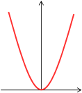
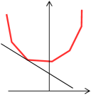
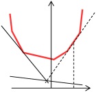
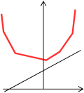
Figure 2: Block-coordinate Frank-Wolfe algorithm for minimizing $\frac{\lambda}{2}||w||^{2}+\sum_{i=1}^{n}H_{i}(w)$ with $n=3$. Each vector $\varphi^{i}$ specifies the current linear lower bound on $H_{i}$. One iteration for term $i=2$ is similar to the classical Frank-Wolfe algorithm, except that the terms $H_{1}$ and $H_{3}$ are approximated by linear lower bounds $\varphi^{1}$ and $\varphi^{3}$, respectively, which are kept fixed during this step.

Algorithm 2 Block-coordinate Frank-Wolfe (BCFW) algorithm for the dual of (1)

1:  for each $i\in[n]$ set $\varphi^{i}\leftarrow\varphi^{iy}$ for some $y\in{\cal Y}$

2:  set $\varphi=\sum_{i=1}^{n}\varphi^{i}$

3:  repeat

4:    pick $i\in[n]$, e.g. uniformly at random

5:    compute $w\leftarrow\operatorname*{arg\,min}_{w}\frac{\lambda}{2}||w||^{2}+\langle\varphi,[w\;1]\rangle$   the solution is given by $w=-\frac{1}{\lambda}\varphi_{\star}$

6:    call $i$-th oracle for vector $w$:   $\hat{\varphi}^{i}\leftarrow\operatorname*{arg\,max}\limits_{\varphi^{iy}:y\in{\cal Y}}\langle\varphi^{iy},[w\;1]\rangle$

7:    compute $\gamma\leftarrow\operatorname*{arg\,max}_{\gamma\in[0,1]}\mathcal{F}(\,\varphi-\varphi^{i}+(1-\gamma)\varphi^{i}+\gamma\hat{\varphi}^{i}\,)$:       set $\gamma\leftarrow\frac{\langle\varphi^{i}_{\star}-\hat{\varphi}^{i}_{\star},\varphi_{\star}\rangle-\lambda(\varphi^{i}_{\circ}-\hat{\varphi}^{i}_{\circ})}{||\varphi^{i}_{\star}-\hat{\varphi}^{i}_{\star}||^{2}}$ and clip $\gamma$ to $[0,1]$

8:    set $\varphi^{i}_{\tt old}\leftarrow\varphi^{i}$,   $\varphi^{i}\leftarrow(1-\gamma)\varphi^{i}+\gamma\hat{\varphi}^{i}$,   $\varphi\leftarrow\varphi+\varphi^{i}-\varphi^{i}_{\tt old}$​​​​

9:  until some stopping criterion

Our main insight is that BCFW acts wastefully by discarding the plane $\hat{\varphi}^{i}$ after completing the iteration for the term $H_{i}$, even though it required an expensive call to the max-oracle to obtain $\hat{\varphi}^{i}$. We propose to retain some of these planes, maintaining a working set ${\cal W}_{i}$ for each $i=1,\dots,n$. We proceed similarly to [16], where a working set was used in a cutting-plane framework. Whenever the oracle for $H_{i}$ is called, the obtained plane $\hat{\varphi}^{i}$ is added to ${\cal W}_{i}$. Planes are removed again from ${\cal W}_{i}$ after a certain time, unless in the mean time they have become active (see below). Consequently, at any iteration the algorithm has access to multiple planes instead of just one, which is why we name the proposed algorithm multi-plane block-coordinate Frank-Wolfe (MP-BCFW).

The working set, ${\cal W}_{i}$, allows us to define an alternative mechanism for increasing the objective value that does not require a call to the costly max-oracle. We define an approximation $\tilde{H}_{i}(w)$ of $H_{i}(w)$ by

$$\tilde{H}_{i}(w)=\max\limits_{\tilde{\varphi}^{i}\in{\cal W}_{i}}\langle\tilde{\varphi}^{i},[w\;1]\rangle.$$ (6)

Note that $\tilde{H}_{i}(w)\leq H_{i}(w)$ for all $w\in\mathbb{R}^{d}$, since the maximization is performed over a smaller set. For any $i\in[n]$, we can perform block updates like in BCFW, but with the term $\tilde{H}_{i}$ instead of $H_{i}$, i.e. in step 5 of Algorithm 2 we set $\hat{\varphi}^{i}\leftarrow\operatorname*{arg\,max}\limits_{\tilde{\varphi}^{i}\in{\cal W}_{i}}\langle\tilde{\varphi}^{i},[w\;1]\rangle$. Such approximate oracle steps will increase $\mathcal{F}(\varphi)$, but potentially less so than a BCFW update using the exact expression.

We propose to interleave the approximate updates steps with exact updates. The order of operations in our current implementation is shown in Algorithm 3. We refer to one pass through the data in lines 5 and 6 as an exact and an approximate pass respectively, and to steps 5-6 as an (outer) iteration. Thus, each iteration contains 1 exact pass and up to $M$ approximate passes. The parameter $N$ bounds the number of stored planes per term: $|{\cal W}_{i}|\leq N$ for each $i$. In this algorithm a plane is considered active at a given moment if is it returned as optimal by either an exact or an approximate oracle call.

The complexity of one approximate update in step 4 is $O(Nd)$, therefore the algorithm performs $O(MNd)$ additional work per each oracle call. For $M=N=0$, MP-BCFW reduces to the classical BCFW algorithm. Since MP-BCFW in particular performs all steps that BCFW does, it inherits all convergence guarantees from the earlier algorithm, such as a convergence rate of $O(\frac{1}{\epsilon})$ towards the optimum, as well as the guarantee of convergence even when the max-oracle can solve the problem only approximately (see [18] for details). However, as we will show in Section 4, MP-BCFW gets more “work done” per iteration and therefore converges faster with respect to the number of max-oracle calls.

Algorithm 3 Multi-Plane Block-Coordinate Frank-Wolfe (MP-BCFW) algorithm. Parameters: $N,M,T$.

1:  for each $i\in[n]$ set $\varphi^{i}\leftarrow\varphi^{iy}$ for some $y\in{\cal Y}$,

2:  set $\varphi=\sum_{i=1}^{n}\varphi^{i}$

3:  if $N>0$  then ${\cal W}_{i}=\{\varphi^{i}\}$ else ${\cal W}_{i}=\varnothing$ for each $i\in[n]$

4:  repeat until some stopping criterion

5:     do one pass through $i\in[n]$ in random order,    for each $i$ do the following:        run BCFW update using original term $H_{i}(w)$        add obtained vector $\hat{\varphi}^{i}$ to ${\cal W}_{i}$        if $|{\cal W}_{i}|\!>\!N$ then remove longest inactive plane from ${\cal W}_{i}$

6:    do up to $M$ passes (see text) through $i\!\in\![n]$ in random order,   for each $i$ do the following:        run BCFW update with term $\tilde{H}_{i}(w)\!=\!\max\limits_{\tilde{\varphi}^{i}\in{\cal W}_{i}}\langle\tilde{\varphi}^{i},[w\;1]\rangle$       remove planes from ${\cal W}_{i}$ that have not been active during        the last $T$ outer iterations

7:  end repeat

3.4 Automatic Parameter Selection

The optimal number of planes to keep per term as well as the optimal number of efficient approximate passes to run depends on several factors, such as the number of support vectors and how far the current solution still is from the optimal one. Therefore, we propose not to set these parameters to fixed values but to adapt them dynamically over time in a data-dependent way. The first criterion described below is fairly standard [16], but the second criterion is specific to MP-BCFW and forms a second contribution of this work.

Working set size.  We observe that the working set is bounded not only by its upper bound parameter, $N$, but also by the mechanism that automatically removes inactive planes. Since the second effect is more interpretable, we suggest to set $N$ to a large value, and rely on the parameter $T$ to control the working set size. In effect, the actual number of planes is adjusted in a data-dependent way for each training instance. In particular, for terms with few relevant planes (support vectors) the working set will be small. A side effect of this is an acceleration of the algorithm, since the runtime of the approximate oracle is proportional to the actual number of planes in their working set.

Number of approximate passes.  We set the maximal number of approximate passes per iteration, $M$, to a large value and rely on the following geometrically motivated criterion instead. After each approximate pass we compute two quantities: 1) the increase in $\mathcal{F}(\varphi)$ per time unit (i.e. the difference of function values divided by the runtime) of the most recent approximate pass, and 2) the increase in $\mathcal{F}(\varphi)$ per unit time of the complete sequence of steps since starting the current iteration. If the former value is smaller than the latter, we stop making approximate passes and start a new iteration with an exact pass.

The above criterion can be understood as an extrapolation of the recent behavior of the runtime-vs-function value graph into the future, see Figure 3. If the slope of the last segment is higher than the slope of the current iteration so far, then the expected increase from another approximate pass is high enough to justify its cost. Otherwise, it is more promising to start a new iteration.

Figure 3: Geometric criterion for number of approximate passes. After each approximate pass, we compare the relative progress (increase in objective per time $=$ slope of the last black line segment) to the relative progress of the complete iteration so far (slope of the dashed line). If the former is higher (left), we make another approximate pass. Otherwise, we start a new iteration (right).

3.5 Weighted averaging of iterates

It has been observed that the convergence speed of stochastic optimization methods can often be improved further by taking weighted averages of iterates [4]. Writing $\varphi^{(k)}$ for the vector produced after the $k$-th oracle call in Algorithm 2 (BCFW), the $k$-th averaged vector is $\bar{\varphi}^{(k)}=\frac{2}{k(k+1)}\sum_{t=1}^{k}t\varphi^{(t)}$. It can also be computed incrementally via $\bar{\varphi}^{(k+1)}=\frac{k}{k+2}\bar{\varphi}^{(k)}+\frac{2}{k+2}\varphi^{(k+1)}$ for $k\geq 1$. Several studies, including [18], has shown that the primal objective of the iterates $\bar{w}^{(k)}=-\frac{1}{\lambda}\bar{\varphi}^{(k)}_{\star}$ often converges to the optimum significantly faster than that of the iterates $w^{(k)}=-\frac{1}{\lambda}\varphi^{(k)}_{\star}$.

For inclusion into MP-BCFW we extended the above scheme by maintaining two vectors, $\bar{\varphi}^{(k)}$ and $\bar{\bar{\varphi}}^{(k^{\prime})}$. They are updated after every exact and after every approximate oracle call, respectively, using the above formula. When we need to extract a solution, we compute the interpolation between $\bar{\varphi}^{(k)}$ and $\bar{\bar{\varphi}}^{(k^{\prime})}$ that gives the best dual objective score. By this construction we overcome the problem that the two types of oracle calls have quite different characteristics, and thus may require different weights.

We refer to the averaged variants of BCFW and MP-BCFW as BCFW-avg and MP-BCFW-avg, respectively.

4 Experiments

We analyze the effectiveness of the MP-BCFW algorithm by performing experiments for four different setting: multi-class classification, sequence labeling, figure-ground segmentation and semantic image segmentation. The first two rely on generic datasets that were used previously to benchmark SSVM training (multi-class classification on the USPS dataset and sequence labeling on the OCR dataset). The third task (figure-ground segmentation on part of the HorseSeg dataset) and the fourth (multiclass semantic image segmentation on the Stanford background dataset) show a typical feature of computer vision tasks: the max-oracle is computationally costly, much more so than in the previous two cases, which results in a strong computational bottleneck for training. In the case of multiclass segmentation the max-oracle is even NP-hard and can be solved only approximately, another common property for computer vision problems. Exact details of dataset characteristics, feature representations and implementation of the oracles for the four datasets are provided in Appendix A.

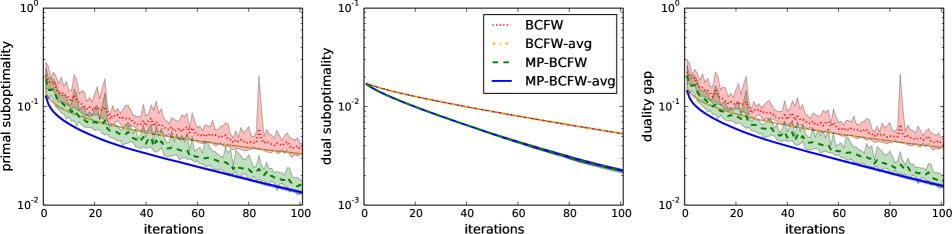
(a) USPS

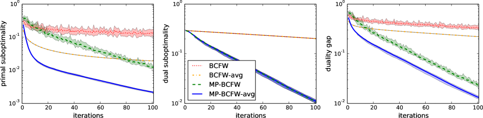
(b) OCR

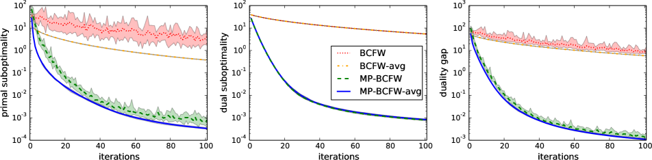
(c) HorseSeg

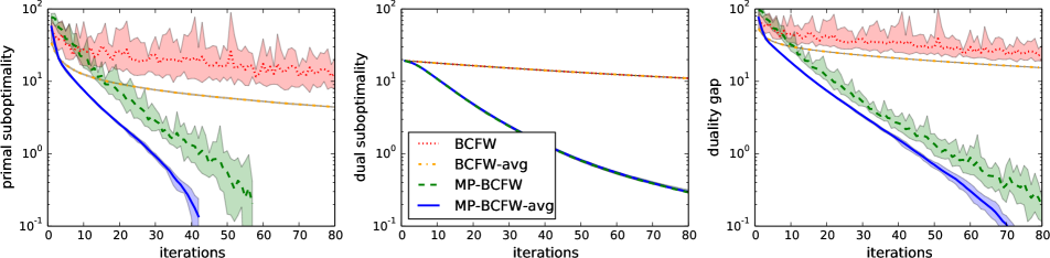
(d) Stanford

Figure 4: Oracle convergence on the four benchmark datasets: primal suboptimality (left), dual suboptimality (middle), duality gap (right). Shaded areas indicate minimum and maximum values over 10 repeats. In all cases, the multi-plane algorithms, MP-BCFW and MP-BCFW-avg, require fewer iterations to reach high quality solutions than the single plane variants, BCFW and BCFW-avg.

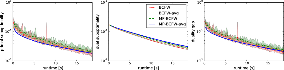
(a) USPS

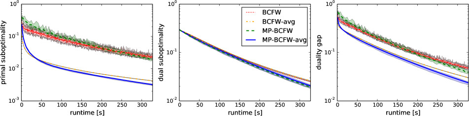
(b) OCR

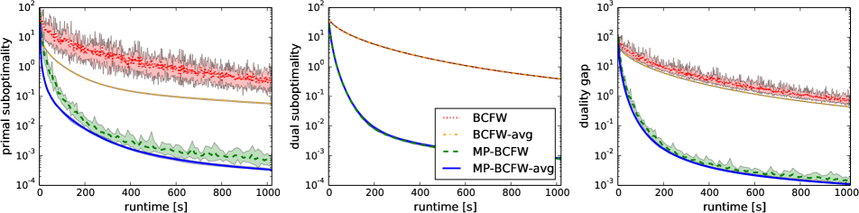
(c) HorseSeg

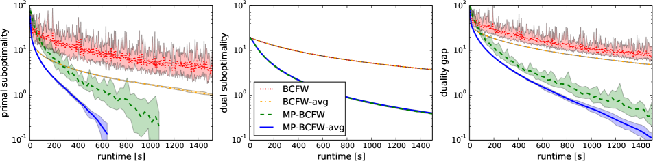
(d) Stanford

Figure 5: Runtime convergence on the four benchmark datasets: primal suboptimality (left), dual suboptimality (middle), duality gap (right). Shaded areas indicate minimum and maximum values over 10 repeats. When the $\max$-oracle is fast (USPS and OCR), the multi-plane algorithms (MP-BCFW, MP-BCFW-avg) behave similarly to their single-plane counterparts (BCFW, BCFW-avg) due to the automatic parameter adjustment. When the $\max$-oracle is computationally costly (HorseSeg, Stanford) the multi-plane variants converge substantially faster.

We focus on comparing MP-BCFW with BCFW (with and without averaging), since in [18] it has already be shown that BCFW offers a substantial improvements over earlier algorithms, in particular classical FW [10], cutting plane training [16], exponentiated gradient [7] and stochastic subgradient training [21]. Since all algorithms solve the same convex optimization problem and will ultimately arrive at the same solution, we are only interested in the convergence speed, not in the error rates of the resulting predictors. This allows us to adopt an easy experimental setup in which we use all available training data for learning and do not have to set aside data for performing model selection. In line with earlier work, we regularize using $\lambda=1/n$.

For all algorithms we measure three quantities: i) the primal suboptimality, i.e. the difference between the primal objective and the highest lower bound we observe during any of our experiments, ii) the dual suboptimality, i.e. the difference between the dual objective and the lowest observed upper bound, and iii) the duality gap, i.e. the difference between the primal and the dual objective. Note that for the Stanford dataset, the reported values are only approximate, since evaluating the objective (1) exactly is intractable. In particular, the primal value is not guaranteed to be an upper bound on the optimal value, so the approximate suboptimalities and duality gap can become negative (at which point we interrupt the logarithmic plots).

We visualize the results in two coordinate frames: i) with respect to the number of iterations, and ii) with respect to the actual runtime. The first quantity, which we refer to as oracle convergence, measures how efficiently the algorithm uses the statistical information that is present in the training examples. It is independent of the implementation and therefore comparable between publications. The second value, called runtime convergence, is of practical interest, because it reflects the computational resources required to achieve a certain solution quality. However, it depends on the concrete implementation and computing hardware. To nevertheless obtain fair runtime comparisons, we use the same code base for all methods, making use of the fact that BCFW can be recovered from MP-BCFW with minimal overhead by deactivating the working sets and approximate passes ($N=0$, $M=0$). For MP-BCFW we rely on the automatic parameter selection mechanism and set $T=10$, $N=1000$, $M=1000$, where the latter two just act as high upper bounds that do not influence the system’s behaviour.

4.1 Results

Figure 4 shows the oracle convergence results for all datasets. One can see that within the same number of iterations (and thereby calls to the max-oracle), MP-BCFW always achieves lower primal suboptimality than BCFW. Similarly, MP-BCFW-avg improves over BCFW-avg.

This effect is stronger for OCR, HorseSeg and Stanford than for USPS, which makes sense, since the latter dataset has a very small label space ($|\mathcal{Y}|=10$), so the number of support vectors per example is small, which limits the benefits of having access to more than one plane. The graph labeling tasks OCR, HorseSeg and Stanford have a larger label spaces, so one can expect more support vectors to contribute to the score. Reusing planes from previous iterations can be expected to have a beneficial effect.

Figure 5 illustrates the runtime convergence, i.e. the values on the vertical axis are identical to Figure 4, but the horizontal axis shows the actual runtime instead of the number of iterations. One can see that for the USPS dataset, the better oracle convergence did not translate to actually faster convergence, and for OCR, the difference between single-plane and multi-plane methods is small.

The situation is different for the HorseSeg and Stanford datasets, which are more typical computer vision tasks. For them, MP-BCFW and MP-BCFW-avg converge substantially faster than BCFW and BCFW-avg. The differences can be explained by the characteristics of the max-oracle in the different optimization problems: for USPS and OCR these are efficient and not do not form major computational bottlenecks. For USPS, the max-oracle requires only computing ten inner products and identifying their maximum. This takes only a few microseconds on modern hardware. Overall, the BCFW algorithm spends approximately 15% of its total runtime on oracle calls. For OCR, the max-oracle is implemented efficiently via Dynamic Programming (Viterbi algorithm), which takes approximate 50µs on our hardware. Overall, oracle calls make up for approximately 70% of BCFW’s runtime. In both settings, the ratio of time spent for the oracle calls and the time spent elsewhere is not high enough to justify frequent use of the approximate oracle.

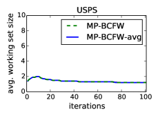
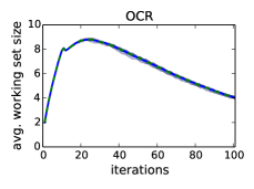
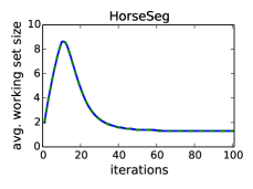
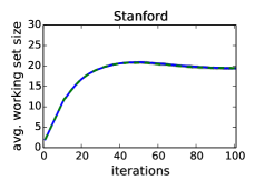
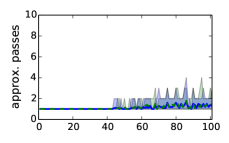
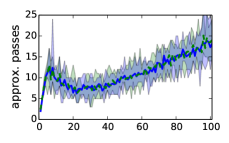
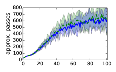
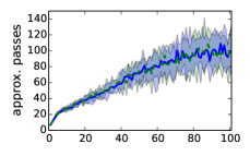
Figure 6: Automatic parameter selection. The size of the working set (top) and the number of approximate passes per iteration (bottom) are adjusted in a data- and runtime-dependent way. See Section 4.2 for details.

Note, however, that even for USPS, MP-BCFW is not slower than BCFW, either. This indicates that the automatic parameter selection does its job as intended: if the overhead of a large working set and many approximate passes would be larger than the benefit they offer, the selection rule falls back to the established (and efficient) baseline behavior.

For the other two datasets, the max-oracle calls are strong computational bottlenecks. For HorseSeg, each oracle call consists of minimizing a submodular energy function by means of solving a maximum flow problem [5]. For the Stanford dataset, the oracle consists of minimizing a Potts-type energy function for which we rely on an efficient preprocessing in [12] followed by the approximation algorithm in [6]. Even with optimized implementations, the oracle calls take 1 to 5 milliseconds, and as a consequence, BCFW spends almost 99% of the total training time on oracle calls. Using MP-BCFW, the fraction drops to less than 25%, because the parameter selection mechanism decides that the time it takes to make one exact oracle call is often spent better for making several approximate oracle calls.

4.2 Automatic parameter selection

Figure 6 illustrates the dynamic behavior of the parameter selection for MP-BCFW in more detail. The first row shows the average size of the working set per term over the course of the optimization, the second row shows the number of approximate passes per iteration.

One can see that for USPS the number of planes and iterations remain small through the runtime of the algorithm, making MP-BCFW behave almost as BCFW. For OCR, the algorithm initially identifies several relevant planes, but this number is reduced for later iterations. The number of approximate passes per iteration ranges between 10 to 15.

For HorseSeg shows a similar pattern but in more extreme form. After an initial exploration phase the number of relevant planes stabilizes at a low value, while the number of approximate passes grows quickly to several hundred. For Stanford, the working set grows steadily to reach a stable state, but the number of approximate passes grows slowly during the course of the optimization.

In summary, one can see that the automatic parameter selection shows a highly dynamic behaviour. It allows MP-BCFW to adapt to the complexity of the objective function as well as to dynamic properties of the optimization, such as how far from the objective the current solution is.

5 Summary and Conclusion

We have presented MP-BCFW, a new algorithm for training structured SVMs that is specifically designed for the situation of computationally costly max-oracles, as they are common in computer vision tasks. The main improvement is the option to re-use previously computed oracle results by means of a per-example working set, and to alternate between calls to the exact but slow oracle and calls to an approximate but fast oracle. We also introduce rules for dynamically choosing the working set size and number of approximate passes depending on the algorithm’s runtime behaviour and its progress towards the optimum. Overall, the result is a easy-to-use method with default settings that work well for a range of different scenarios. Our C++ implementation is publicly available at [1].

Our experiments showed that MP-BCFW always requires fewer iterations to reach a certain solution quality than the BCFW algorithm, which had previously been shown to be superior to earlier methods. This leads to faster convergence towards the optimum for situations in which the max oracle is the computational bottleneck, as it is typical for structured learning tasks in computer vision.

In future work we plan to explore the situation of very high-dimensional or kernelized SSVMs, where a further acceleration can be expected by precomputing and caching inner product evaluations.

Appendix A Details of Datasets and max-Oracles

We give details of the four different applications scenarios with max-oracles of increasing complexity.

Multiclass Classification – USPS Dataset

The USPS dataset is a standard multiclass dataset with 7291 samples of 10 classes, $\mathcal{Y}=\{\texttt{0},\texttt{1},\dots,\texttt{9}\}$. Each sample, $x$, comes with a 256-dimensional feature vector, $\psi(x)$, from which we build a 2560-dimensional joint feature map

$$\phi(x,y)=\Big{(}\psi(x)\llbracket y=\texttt{0}\rrbracket,\dots,\psi(x)\llbracket y=\texttt{9}\rrbracket\Big{)}.$$ (7)

As loss function we use the ordinary multiclass loss, $\delta(y,\bar{y})=\llbracket y\neq\bar{y}\rrbracket$. Overall, the structured Hinge loss is

$$H_{i}(w)=\frac{1}{n}\max_{y\in\mathcal{Y}}\Big{\{}\ \llbracket y_{i}\neq y\rrbracket+\big{\langle}\,w,\phi(x_{i},y)-\phi(x_{i},y_{i})\,\big{\rangle}\ \Big{\}}$$ (8)

Because of the small label set the max oracle can be performed efficiently by an explicit search over all labels.

Sequence Labeling - OCR dataset

The OCR dataset consists of 6877 data samples that are sequences of hand-written letters, $x=(x^{1},x^{2},\dots,x^{L})$, where for each part, $x^{l}$, a feature vector $\psi(x^{l})\in\mathbb{R}^{128}$ is available. The outputs are sequences of labels, $y=(y^{1},y^{2},\dots,y^{L})$ of the same length, where $y^{l}\in\{\texttt{a},\dots,\texttt{z}\}$ for each $l=1,\dots,L$. The length of the sequences in fact differs for different examples with an average of 7.6. We do not indicate this explicitly in order to keep the notation simple.

We define a joint feature map, $\phi(x,y)=\big{(}\phi_{u}(x,y),\phi_{p}(x,y)\big{)}$, consisting of a unary and a pairwise component:

$$\phi_{u}(x,y)=\sum_{l=1}^{L}\phi(x^{l},y^{l}),\qquad\phi_{p}(x,y)=\sum_{l=1}^{L-1}e_{y^{l},y^{l+1}},$$

where $\phi(x_{l},y_{l})$ is a multiclass encoding of the feature $\psi(x_{l})$ as defined above for the USPS dataset, and $e_{a,b}$ is the $26^{2}$-dimensional binary vector indicating the label pair $(a,b)$ out of all possible label transitions. As loss function we use the normalized Hamming loss, $\Delta(y,\bar{y})=\frac{1}{L}\sum_{l=1}^{L}\llbracket y^{l}\neq\bar{y}^{l}\rrbracket$.

The structured Hinge loss can be written using a summation over all positions and transitions:

$$H_{i}(w) = \frac{1}{n}\max_{y\in\mathcal{Y}}\Big{\{}\sum_{l=1}^{L}\frac{1}{L}\llbracket y^{l}_{i}\neq y^{l}\rrbracket$$ (9)

$$+\langle\,w_{u},\phi(x^{l}_{i},y^{l})-\phi(x^{l}_{i},y^{l}_{i})\,\rangle$$

$$+\sum_{l=1}^{L-1}\langle\,w_{p},e_{y^{l},y^{l+1}}-e_{y^{l}_{i},y^{l+1}_{i}}\,\rangle\ \Big{\}},$$

where $w=(w_{u},w_{p})$ is a decomposition of the weight vector into parts acting on the unary and pairwise part of the joint feature map, accordingly. Even though the size of the label space grows exponentially in the length of the sequence, $|\mathcal{Y}|=26^{L}$, the additive structure of the problem makes it possible to solve the max-oracle efficiently using dynamic programming, namely by the Viterbi algorithm [27].

Image Segmentation – HorseSeg Dataset and Stanford Backgrounds Dataset

We use a subset of 2376 image of the HorseSeg dataset [17], and the 715 images of the Stanford Backgrounds dataset [11], respectively. First, each image, $x$, is decomposed into a variable number of superpixels, $x^{1},\dots,x^{L}$, using the SLIC method [2]. Then, each superpixel is represented by a 649-dimensional feature vector $\phi(x^{l})$. The task consists of predicting a segmentation, $y=(y^{1},\dots,y^{L})$, for each image. For the HorseSeg dataset, this is a figure-ground mask, i.e. each superpixel is assigned binary, $y^{l}\in\{0,1\}$ for every $l=1,\dots,L$. For the Stanford dataset, each superpixel is assigned one of nine semantic class labels, $y^{l}\in\{1,\dots,9\}$ for every $l=1,\dots,L$.

We construct a joint feature map using the same construction as for the unary term in the OCR dataset,

$$\phi(x,y)=\sum_{l=1}^{L}\phi(x^{l},y^{l}),$$

where $\phi$ is defined by Equation (7). In addition, we add a pairwise term of Potts type to the SSVM prediction function,

$$\Theta(x,y)=\sum_{k\sim l}\llbracket y^{k}\neq y^{l}\rrbracket$$

where $k\sim l$ denotes that the superpixels $k$ and $l$ are neighbors in the image. For this term, we do not learn a weight vector, but assign it a constant weight of $1$. Formally, the term therefore is not part of the feature vector but contributes to the $\varphi_{\circ}$ component of the parameterization (see Section 3 of the main manuscript).

As loss function we again use the normalized Hamming loss and we obtain the following structured Hinge loss

$$H_{i}(w) = \frac{1}{n}\max_{y\in\mathcal{Y}}\Big{\{}\sum_{l=1}^{L}\frac{1}{L}\llbracket y^{l}_{i}\neq y^{l}\rrbracket$$ (10)

$$+\langle\,w_{u},\phi(x^{l}_{i},y^{l})-\phi(x^{l}_{i},y^{l}_{i})\,\rangle$$

$$+\sum_{k\sim l}\llbracket y^{k}\neq y^{l}\rrbracket\ \Big{\}}.$$

For HorseSeg, the objective in this discrete optimization is submodular, and we implement the max-oracle using the mincut algorithm [5]. For Stanford, the resulting optimization function is NP-hard in general. As max-oracle we use an approximation given by the alpha-expansion algorithm [6] combined with an efficient preprocessing from [12].

References

- [1] http://pub.ist.ac.at/~vnk/papers/SVM.html. Our implementation of MP-BCFW.
- [2] R. Achanta, A. Shaji, K. Smith, A. Lucchi, P. Fua, and S. Süsstrunk. SLIC superpixels compared to state-of-the-art superpixel methods. IEEE Transactions on Pattern Analysis and Machine Intelligence (PAMI), 34(11):2274–2282, 2012.
- [3] L. Bertelli, T. Yu, D. Vu, and B. Gokturk. Kernelized structural SVM learning for supervised object segmentation. In IEEE Conference on Computer Vision and Pattern Recognition (CVPR), 2011.
- [4] L. Bottou. Stochastic gradient descent tricks. In Neural Networks: Tricks of the Trade, pages 421–436. 2012.
- [5] Y. Boykov and V. Kolmogorov. An experimental comparison of min-cut/max-flow algorithms for energy minimization in vision. IEEE Transactions on Pattern Analysis and Machine Intelligence (PAMI), 26(9):1124–1137, 2004.
- [6] Y. Boykov, O. Veksler, and R. Zabih. Fast approximate energy minimization via graph cuts. IEEE Transactions on Pattern Analysis and Machine Intelligence (PAMI), 23(11), 2001.
- [7] M. Collins, A. Globerson, T. Koo, X. Carreras, and P. L. Bartlett. Exponentiated gradient algorithms for conditional random fields and max-margin Markov networks. Journal of Machine Learning Research (JMLR), 9:1775–1822, 2008.
- [8] C. Cortes and V. Vapnik. Support-vector networks. Machine learning, 20(3):273–297, 1995.
- [9] J. Deng, W. Dong, R. Socher, L.-J. Li, K. Li, and L. Fei-Fei. ImageNet: A Large-Scale hierarchical image database. In IEEE Conference on Computer Vision and Pattern Recognition (CVPR), 2009.
- [10] M. Frank and P. Wolfe. An algorithm for quadratic programming. Naval Research Logistics Quarterly, 3:149–154, 1956.
- [11] S. Gould, R. Fulton, and D. Koller. Decomposing a scene into geometric and semantically consistent regions. In IEEE International Conference on Computer Vision (ICCV), 2009.
- [12] I. Gridchyn and V. Kolmogorov. Potts model, parametric maxflow and -submodular functions. In IEEE International Conference on Computer Vision (ICCV), 2013.
- [13] A. Gupta, M. Hebert, T. Kanade, and D. M. Blei. Estimating spatial layout of rooms using volumetric reasoning about objects and surfaces. In Conference on Neural Information Processing Systems (NIPS), 2010.
- [14] S. Hare, A. Saffari, and P. H. Torr. Struck: Structured output tracking with kernels. In IEEE International Conference on Computer Vision (ICCV), 2011.
- [15] C. Ionescu, L. Bo, and C. Sminchisescu. Structural SVM for visual localization and continuous state estimation. In IEEE International Conference on Computer Vision (ICCV), 2009.
- [16] T. Joachims, T. Finley, and C. Yu. Cutting-plane training of structural SVMs. Machine Learning, 1:27–59, 2009.
- [17] A. Kolesnikov, M. Guillaumin, V. Ferrari, and C. H. Lampert. Closed-form approximate crf training for scalable image segmentation. In European Conference on Computer Vision (ECCV), 2014.
- [18] S. Lacoste-Julien, M. Jaggi, M. Schmidt, and P. Pletscher. Block-coordinate Frank-Wolfe optimization for structural SVMs. In International Conference on Machine Learning (ICML), 2014.
- [19] X. Lou and F. A. Hamprecht. Structured learning for cell tracking. In Conference on Neural Information Processing Systems (NIPS), 2011.
- [20] S. Nowozin, P. V. Gehler, and C. H. Lampert. On parameter learning in CRF-based approaches to object class image segmentation. In European Conference on Computer Vision (ECCV), 2010.
- [21] N. D. Ratliff, J. A. Bagnell, and M. A. Zinkevich. (Online) subgradient methods for structured prediction. In Conference on Uncertainty in Artificial Intelligence (AISTATS), 2007.
- [22] A. G. Schwing, T. Hazan, M. Pollefeys, and R. Urtasun. Efficient structured prediction for 3d indoor scene understanding. In IEEE Conference on Computer Vision and Pattern Recognition (CVPR), 2012.
- [23] M. Szummer, P. Kohli, and D. Hoiem. Learning CRFs using graph cuts. In European Conference on Computer Vision (ECCV), 2008.
- [24] B. Taskar, C. Guestrin, and D. Koller. Max-margin Markov networks. In Conference on Neural Information Processing Systems (NIPS), 2004.
- [25] C. H. Teo, S. Vishwanthan, A. J. Smola, and Q. V. Le. Bundle methods for regularized risk minimization. Journal of Machine Learning Research (JMLR), 11:311–365, 2010.
- [26] I. Tsochantaridis, T. Joachims, T. Hofmann, and Y. Altun. Large margin methods for structured and interdependent output variables. Journal of Machine Learning Research (JMLR), 6:1453–1484, 2005.
- [27] A. J. Viterbi. Error bounds for convolutional codes and an asymptotically optimum decoding algorithm. IEEE Transactions on Information Theory,, 1967.
- [28] W. Yang, Y. Wang, and G. Mori. Recognizing human actions from still images with latent poses. In IEEE Conference on Computer Vision and Pattern Recognition (CVPR), 2010.