Optimal control theory with arbitrary superpositions of waveforms

Abstract

Standard optimal control methods perform optimization in the time domain. However, many experimental settings demand the expression of the control signal as a superposition of given waveforms, a case that cannot easily be accommodated using time-local constraints. Previous approaches [1, 2] have circumvented this difficulty by performing optimization in a parameter space, using the chain rule to make a connection to the time domain. In this paper, we present an extension to Optimal Control Theory which allows gradient-based optimization for superpositions of arbitrary waveforms directly in a time-domain subspace. Its key is the use of the Moore-Penrose pseudoinverse as an efficient means of transforming between a time-local and waveform-based descriptions. To illustrate this optimization technique, we study the parametrically driven harmonic oscillator as model system and reduce its energy, considering both Hamiltonian dynamics and stochastic dynamics under the influence of a thermal reservoir. We demonstrate the viability and efficiency of the method for these test cases and find significant advantages in the case of waveforms which do not form an orthogonal basis.

1 Introduction

Optimal control theory aims at driving a dynamical system towards a final state that minimizes a figure of merit and at finding the required time-dependent controls. In classical physical systems, optimal control schemes have been used successfully for decades [3, 4], and for some time various optimal control algorithms have been applied to a wide range of quantum systems, see e.g. [5, 6, 7, 8, 9, 10]. There is a renewed interest in applying and improving established algorithms like the Krotov algorithm [11] or gradient methods [12], and new control techniques are being developed for control problems of increasing complexity [13, 14, 15, 16].

Speed-up of optimization is often achieved by restriction of the control pulses to certain pulse families, such as, e.g., Gaussian pulse cascades [17] or Fourier expansions [18, 19, 20, 21]. Also, more elaborate ways of truncating the search space have been formulated, like e.g. the CRAB algorithm [16]. These methods are especially successful, if the underlying dynamics is well known and understood, which allow for a sophisticated choice of the basis functions. Additionally, the comparatively easy shape of the pulse (limited, e.g., to a few frequency components only), allows for a straight forward interpretation.

In order to gain experimentally realizable control pulses, additional constraints may have to be taken into account, such as restricting the total energy or limiting the control functions [12, 13, 22, 23, 24, 25, 26]. Not all control algorithms follow this requirement equally well; for the effects such constraints have on the convergence behaviour of control algorithms, see [2]. Methods to design pulse shapes as analytic functions of a small set of parameters have been introduced [1], which allow restrictions on the shape of the control pulse. The most elementary extension of gradient-based control theory to this scenario consists in simply applying the chain rule of calculus.

In this paper we present a control algorithm which takes similar experimental constraints into account, while working in a proper subspace of actual functions of time rather than a parameter space. Our control subspace is defined from linear combinations of arbitrary waveforms. The properties of orthogonality, normalization, or even linear independence are not required in our case, valid solutions in the time domain are obtained in either case.

The method is tested by examining a generic model system, for which methods of comparison are available. However, the method is not restricted to such simple systems, but, as in section 2 described, broadly applicable.

The paper is organized as follows: In section 2 the general method is described which is then applied to generic test cases in section 3, including a discussion of performance characteristics. A short summary together with an outline of potential extensions and applications follow in section 4.

2 Method: experimentally realizable control functions

The aim is to control a dynamical system with an equation of motion $\dot{\bi{z}}=f(\bi{z}(t),u(t))$, where $z(t)$ is the dynamical state vector, and $u(t)$ is an external time-dependent control. An optimal control function $u(t)$ is sought which changes the dynamics of the system towards a desired property of a final state at given time $\tau$. The objective can be quantified by a cost functional $\Phi[\bi{z}(\tau)]$. For the sake of clarity, only a scalar control signal $u(t)$ is considered; but this is easily generalized to the case of multiple control variables. To find the optimal control function $u(t)$, which also considers the constraint that the equations of motion needs to be satisfied, an extremum of the augmented cost functional

$$J[u(t)]=\Phi[\bi{z}(\tau)]+\int\limits_{t_{i}}^{\tau}\bi{\lambda}^{t}(t)\{\dot{\bi{z}}(t)-f(\bi{z}(t),u(t))\}dt,$$ (1)

needs to be determined. $\bi{\lambda}(t)$ denotes a vector of Lagrange multipliers.

Variational calculus on (1) yields equations of motion also for the Lagrange multipliers, which are therefore referred to as co-states. Variation of the system state at the final time yields a final-time boundary condition for the co-state, which depends on the final-time value of the state variable $\bi{z}(\tau)$. Furthermore, variation with respect to $u(t)$ leads to the gradient

$$\quad\frac{\partial J}{\partial u(t)}=-\bi{\lambda}^{t}(t)\frac{\partial f}{\partial u}.$$ (2)

The optimal control function $u(t)$ can then be found by searching for zeros of this gradient. For solving optimal control problems gradient methods are well established [3, 12]. As computing the gradient is relatively cheap (only twice the effort of a simple evaluation of the cost functional), it is almost always favourable to adopt an optimization technique which makes use of the information supplied by the gradient to determine the direction and width of the search step for the next optimization iteration. The method presented here is therefore based on a gradient method.

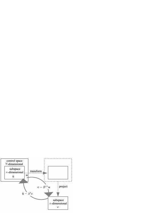
Figure 1: Schematic representation of the function spaces in which the optimization problem can be formulated. In full control space (big box in the upper left) the time discretized control pulse is a $N$-dimensional vector $\bi{u}$. An $n$-dimensional subspace (inset, top left), spanned by vectors combined in a matrix $B$, the control pulse may be described by a $n$-dimensional coefficient vector $\bi{c}$ (bottom). After transforming to the subspace and back, $\bi{u}$ is not recovered, but $\bi{\widetilde{u}}$, a time dependent vector in the $n$-dimensional subspace. Note that a direct transformation (curved down arrow) based on the Moore-Penrose pseudoinverse $B^{+}$ performs both a projection and a change of representation in one step.

The numerical representation of the control function $u(t)$ is, due to the discrete time steps $\delta t$, a $N$-dimensional vector:

$$u(t)\rightarrow(u(t_{1}),\ldots,u(t_{k}),\ldots,u(t_{N})),\quad t_{k}=k\cdot\delta t,\quad k=1,\ldots,N,$$ (3)

with $\tau\equiv t_{N}$, $t_{i}\equiv t_{1}$ and in shorter notation $u(t)\rightarrow(u_{1},\ldots,u_{k},\ldots,u_{N})\equiv\bi{u}^{t}$. With the dynamics as an implied constraint, the cost to be optimized becomes a functional $\Phi[\bi{u}]$. The underlying $N$-dimensional function space will be called full function space or control space.

However, depending on the problem under study, additional constraints for the control function $u(t)$, the dynamical variable $\bi{z}(t)$ or a function $\mathcal{E}(\bi{z},u,t)$ may be required. Hard boundaries for the variables just mentioned can be expressed as inequality conditions $\mathcal{E}(\bi{z},u,t)>0$. There are different approaches to consider these restrictions: Either additional Lagrange terms in the augmented cost functional (1) are included in the formalism or a suitable change of variables is performed. For details see [13, 22, 23]. Another way is to take into account additional cost functionals of the form $J_{add}[u(t)]=\alpha\int\limits_{t_{i}}^{\tau}dt\Theta[\mathcal{E}(\bi{z},u,t)]$, where $\Theta$ denotes the Heaviside-function and $\alpha$ is a parameter to give priority to this constraint. A large enough value of $\alpha$ enforces the restriction, but there is no guarantee that it will not be violated for brief periods of time, when using additional cost functionals.

On the other hand, an important, experimentally relevant class of constraints cannot be expressed through inequality constraints or an additional time-local term in the cost functional. E.g, pulse shapes available for optical control signals are often characterized by a set of parameters determining a pulse sequence through central frequencies and shape parameters. Such constraints could be expressed through equations involving functionals of the control signal, however, we are going to take the simpler, more transparent approach of working in the lower-dimensional (truncated) function space implied by the parametrization. Note that this is subtly different from working directly in the parameter space [1]: Even if both spaces share the same affine structure, their natural scalar products, which are used in numerical optimization, are rarely identical.

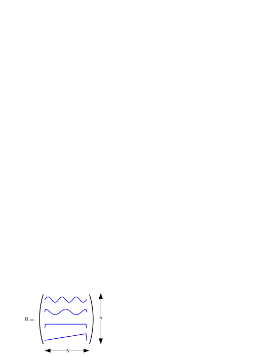
Figure 2: (color online) Schematic representation of the Matrix $B$ (4) with rows determined by the waveforms $b_{l}(t)$ or their vector equivalents $\bi{b}_{l}^{t}$. The transpose $B^{t}$ transforms a coefficient vector $\bi{c}$ into a control function $\bi{u}$, see equation (6). $B$ is not square, typically $n\ll N$. The vectors $\bi{b}_{l}$ representing the waveforms need not to be orthogonal.

In this paper we present a method to take into account the type of constraint implied by a parametrization of the control $u(t)$ as the superposition of $n$ experimentally realizable waveforms $b_{l}(t)$ (cf. figure 1). The functions $b_{l}(t)$ can be interpreted as vectors, defining a linear space through their span. This space is obviously a subspace of the space of control functions $u(t)$ admissible in the absence of constraints. In the numerical representation, we get $N$-dimensional vectors $\bi{b}_{l}$. These vectors form an $n\times N$ matrix

$$B=\left(\begin{array}[]{c}\bi{b}_{1}^{t}\\ \vdots\\ \bi{b}_{n}^{t}\end{array}\right),$$ (4)

which can be used to tranform the coefficient vector $\{c_{1},\ldots c_{l},\ldots,c_{n}\}\equiv\bi{c}^{t}$ of a superposition of waveforms into the time domain, i.e., the superposition

$$\widetilde{u}(t)=\sum\limits_{l=1}^{n}c_{l}b_{l}(t)$$ (5)

can be written in the compact form

$$\bi{\widetilde{u}}=B^{t}\bi{c}.$$ (6)

The matrix $B$ is schematically shown in figure 2.

The optimization now consists in the task of finding a control $\bi{\widetilde{u}}$ within the subspace for which $\Phi[\bi{\widetilde{u}}]$ is at an extremum. We shall see below that this is feasible without placing any restrictions on the vectors $\{\bi{b}_{l}\}$. Note that the $\{\bi{b}_{l}\}$ need not be linearly independent, in particular they need not be normalized or orthogonal, but we may choose them normalized for convenience.

Lack of any restrictions on the vectors $\{\bi{b}_{l}\}$ makes our approach highly flexible. Functions $\{b_{l}(t)\}$ with arbitrary shapes may be chosen - symmetric or asymmetric pulses, ramps and plateaus, chirped pulses, virtually anything a given application may require. Since orthogonality is not a criterion, pulse shapes can also easily be modified for smooth rise or fall to/from an initial or final value of zero.

Now we want to minimize $\Phi[\bi{\widetilde{u}}]$ with the aid of the gradient (2). The gradient can be calculated by first solving the equation of motion for the system degrees of freedom $\dot{\bi{z}}=f(\bi{z},\widetilde{u})$. Then the final time value $\bi{z}(\tau)$ fixes the end-time value of the Lagrange multiplier, which can be propagated backwards in time to get the solution $\bi{\lambda}(t)$. This is the standard computational approach to obtain the gradient (2). In the present context, the equations of motion and the gradient depend on the truncated control $\bi{\widetilde{u}}$, as the optimization is performed in the subspace. However, the gradient vector obtained from (2) typically lies outside the subspace of interest, it needs to be projected back each time it is computed. It is therefore essential to find an efficient way to perform this projection as well as the transformations between the time domain and the coefficients of the waveform decomposition.

Since the waveforms cannot be assumed to be orthogonal functions, the transformation cannot be performed using a simple scalar product

$$c_{l}=\bi{u}\cdot\bi{b}_{l}\quad\not\Leftrightarrow\quad\bi{\widetilde{u}}=\sum\limits_{l=1}^{n}c_{l}\bi{b}_{l}.$$ (7)

This also means that $\sum\limits_{l}\bi{b}_{l}^{t}\cdot\bi{b}_{l}$ cannot be used as a projector on the constrained subspace, which would be the case for an orthonormal basis. Moreover, if the $\{\bi{b}_{l}\}$ are not linearly independent, the coefficients $c_{l}$ are not unique. However, we shall demonstrate below that even in this case the constrained optimization problem is well-defined and converges to unambiguous solutions $\widetilde{u}(t)$.

Even for the case of linearly independent $\{\bi{b}_{l}\}$, completing the matrix $B$ into a quadratic matrix with full rank, computing its inverse and performing a projection onto the subspace (dotted indirect path in 1) would generally be much more tedious than the method we introduce here.

To be able to perform the transformation with ease, we suggest the use of the Moore-Penrose-Pseudoinverse $B^{+}$ [27] (PINV). It has the following defining properties:

$$\eqalign{BB^{+}B=&B\qquad\quad\;B^{+}BB^{+}=B^{+}\cr(BB^{+})^{*}=&BB^{+}\qquad(B^{+}B)^{*}=B^{+}B.}$$ (8)

$B^{+}$ exists for any matrix $B$. Both $B^{+}B$ and $BB^{+}$ are projection matrices. This definition contains the ordinary inverse as a special case, where $B^{+}B=BB^{+}=\mathds{1}$. The equations

$$\bi{c}=B^{t+}\bi{u}\quad\mbox{and}\quad\bi{\widetilde{u}}=B^{t}\bi{c}=B^{t}{B^{t+}}\bi{u}=B^{+}B\bi{u}$$ (9)

provide all the required transformations and projections (see figure 1).

When transforming back to the time domain in the case $n<N$, it is not necessarily the original vector $\bi{u}$ that is recovered, but $\bi{\widetilde{u}}$, which is the result of the projection $B^{+}B$. This is exactly what is required for a consistent iterative optimization in the subspace. Suitable algorithms for the precise and efficient computation of the pseudoinverse exist and are implemented in many numerical libraries and software packages.

We are now in a position to formulate an iteration scheme which computes a solution of the constrained control problem while making use of the gradient of the objective functional in the full space, which can be obtained from the dynamics of states and co-states. Now the following step-by-step instruction for the PINV method can be given:

1. Define the cost functional and choose the generating system $\{\bi{b}_{l}\}$ for the subspace. Choose an initial guess $\bi{u_{i}}$ for the optimal control pulse.

2. Compute the values of the cost functional and the gradient and project the gradient on the subspace:

   $$J[\bi{\widetilde{u}}_{i}]=J[B^{+}B\bi{u}_{i}]$$ (10)

   $$\nabla_{\widetilde{u}}J[\bi{\widetilde{u}}_{i}]=B^{+}B\,\nabla_{u}J[\bi{u}]|_{\bi{u}=\bi{\widetilde{u}}_{i}}.$$ (11)

   $\nabla_{u}$ denotes the gradient with respect to $\bi{u}$.

3. Perform the optimization search step, e.g., a line search, in the $n$-dimensional subspace. This can be done by a “black box” routine implementing standard optimization techniques. In most cases, one thus finds a control signal $\bi{\widetilde{u}}_{i+1}$ with $J[\bi{\widetilde{u}}_{i+1}]<J[\bi{\widetilde{u}}_{i}]$.

4. Set $\bi{u}_{i}=\bi{\widetilde{u}}_{i+1}$ and start again at step (ii) until $J[\bi{\widetilde{u}}_{i}]-J[\bi{\widetilde{u}}_{i+1}]<\epsilon$, where the parameter $\epsilon$ then defines the convergence criterion.

Using these steps, both the gradient search and conjugate gradient algorithms as well as quasi-Newton optimization algorithms [28, 29, 30] can be adapted to perform optimal control in a parameter subspace. The latter algorithms use values of the gradient from several iteration cycles to build an approximate Hessian matrix to accelerate convergence.

3 Test cases and results

As a proof of concept, we apply our method to two simple model systems, for which comparison data can easily be obtained. In order to show the flexibility of the tested PINV method and the compatibility with different optimization algorithms, the results presented here are computed using different gradient-based optimization methods. In section 3.1 a L-BFGS quasi-Newton method [30] and in section 3.2 a steepest descent algorithm will be used.

3.1 Control of deterministic dynamics

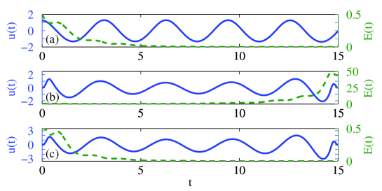
Figure 3: (color online) The control signals (blue solid lines, dimensionless units on left axes) and the energies of the controlled system (green dashed lines, right axes). Data in (a) correspond to the optimization in full function space with final-time energy $E(\tau)=2.850\cdot 10^{-5}$. In (b) this control is truncated to a $n=12$-dimensional subspace defined in (14). This post-truncated control leads to $E(\tau)=44.096$. In (c) the result achieved with the PINV method in the same subspace as in (b) is shown. Using this control function one achieves $E(\tau)=4.432\cdot 10^{-6}$

.

The system of interest for this section is a parametrically driven harmonic oscillator. Its dynamics is described by the set of differential equations

$$\eqalign{\dot{q}&=\frac{p}{m}\cr\dot{p}&=-m\omega_{0}^{2}q(t)-u(t)q(t)}$$ (12)

with a parametric control function $u(t)$. For convenience, we set $\omega_{0}=1$ and $m=1$ in the following (natural units) and choose an initial state $(q_{0},p_{0})=(1/\sqrt{2},1/\sqrt{2})$ with initial energy $E(0)=0.5$. The control objective is the minimization of energy at the fixed final time $\tau=15$, i.e.

$$\Phi[q(\tau),p(\tau)]=\frac{q^{2}(\tau)}{2}+\frac{p^{2}(\tau)}{2}.$$ (13)

As generating set for the subspace in which the optimization will be performed we choose the following (non-orthogonal) functions

$$\left.\begin{array}[]{c}b_{l}(t)=\frac{1}{\mathcal{N}}e(t)\sin\left(\frac{2\pi}{\tau}l\cdot t\right)\\ \\ b_{l+\frac{n}{3}}(t)=\frac{1}{\mathcal{N}}e(t)\cos\left(\frac{2\pi}{\tau}l\cdot t\right)\\ \\ b_{l+\frac{2n}{3}}(t)=\frac{1}{\mathcal{N}}e(t)t^{l-1}\end{array}\right\}\quad l=1,\cdots,\frac{n}{3}$$ (14)

on $[0,\tau]$ with a scaling constant $\mathcal{N}$ and an envelope function $e(t)$ enforcing initial and final values $b_{k}(0)=b_{k}(\tau)=0$, modeled on the finite time needed to switch a real-world pulse. The function $e(t)$ rises from zero to unity within a specified time interval $[0,t_{0}]$, followed by a plateau and a symmetric decline in the interval $[\tau-t_{0},\tau]$. For the initial rise, $t\in[0,t_{0}]$, we choose

$$e(t)=\frac{1}{2}\left\{1+\tanh\left[\frac{\eta\cdot y(t)}{1-y(t)^{4}}\right]\right\},$$ (15)

with $y(t)=\frac{2t}{t_{0}}-1$ and the parameters $t_{0}=0.5$ and $\eta=2$. Note that $e(t)$ is smooth at $t=t_{0}$ and $t=\tau-t_{0}$, all its derivatives are zero at these points. The matrix $BB^{t}$, which is the unit matrix in the case of an orthonormal basis, has widely differing eigenvalues in our case; its condition number is approximately $1.3\cdot 10^{8}$.

In figure 3 the control functions (blue solid lines) and the corresponding energies (green dashed lines) are shown for three different approaches to optimal control. The top panel displays results for optimization in the full space. Using the L-BFGS quasi-Newton algorithm [30], a solution with a very small final energy $E(\tau)=2.850\cdot 10^{-5}$ is computed. (Since this is a fully controllable system, the exact solution is zero). As might be expected for parametric control, the dominant frequency of this control is twice the system frequency $2\omega_{0}$, which can be qualitatively understood as follows: When the particle is in the minimum of the potential, the control makes the potential well narrower, decreasing its amplitude after traversing the minimum. When the particle is near the turning points, the potential is opened to extract energy.

In panel (b) of figure 3, the control pulse optimized in full function space [panel (a)] is truncated to the subspace after the iteration has been performed, instead of using the PINV scheme described in section 2. The basis functions are given by (14) with $n=12$. Although the truncated control signal still looks fairly similar to the original one, the dynamics results in a huge final-state energy. (Note the different scales). The naive post-optimization truncation shown here is definitely not a viable approach to control theory with superpositions of waveforms. In the bottom panel (c) the control pulse is determined using the PINV-based approach described in section 2, applying it to the L-BFGS algorithm [30]. The same subspace as in panel 3(b) is used, however, the final energy $E(\tau)=4.432\cdot 10^{-6}$ is also very close to the exact result. The initial guess for the control is $\bi{u}_{i}=0$, and the convergence parameter is set to $\epsilon=10^{-6}$ for all runs shown in figure 3.

3.2 Control of an open system at finite temperature

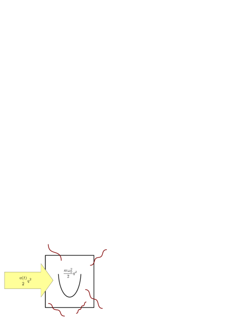
Figure 4: (color online) Schematic representation of the system under study in section  3.2 and 3.3. A harmonic oscillator is coupled to a thermal environment, see text for details. The arrow illustrates the external parametric control.

In this section we look again at a harmonic oscillator ($\omega_{0}=1,m=1$), but now in contact with an environment in thermal equilibrium at temperature $T$ as illustrated in figure 4.

A general description for open classical systems is the Langevin equation [31], which reads for the system under study (with parametric control)

$$\eqalign{\dot{q}(t)=&\frac{p}{m}\cr\dot{p}(t)=&-m\omega_{0}^{2}q(t)-\int\limits_{0}^{t}ds\gamma(t-s)\dot{q}(s)-u(t)q(t)+\xi(t),}$$ (16)

where the stochastic force $\xi(t)$ satisfies the Fluctuation-Dissipation Theorem, $\langle\xi(t)\xi(t^{\prime})\rangle=mk_{\rm B}T\gamma(t-t^{\prime})$ for $t>t^{\prime}$. We assume a Drude damping for the environment associated with a friction-kernel

$$\gamma(t)=\gamma_{0}\omega_{c}\Theta(t)e^{-\omega_{c}t},$$ (17)

with damping constant $\gamma_{0}$ and cut-off frequency $\omega_{c}$. The parameters are set to $\gamma_{0}=0.1$, $\omega_{c}=10$ and $k_{\rm B}T=1$.

Based on this description valid for single noise realizations $\xi(t)$, the expectation value $\mbox{I\negthinspace E}[\cdot]$ is estimated by taking the average of many realizations. The presented results are achieved with $M=1000$ realizations.

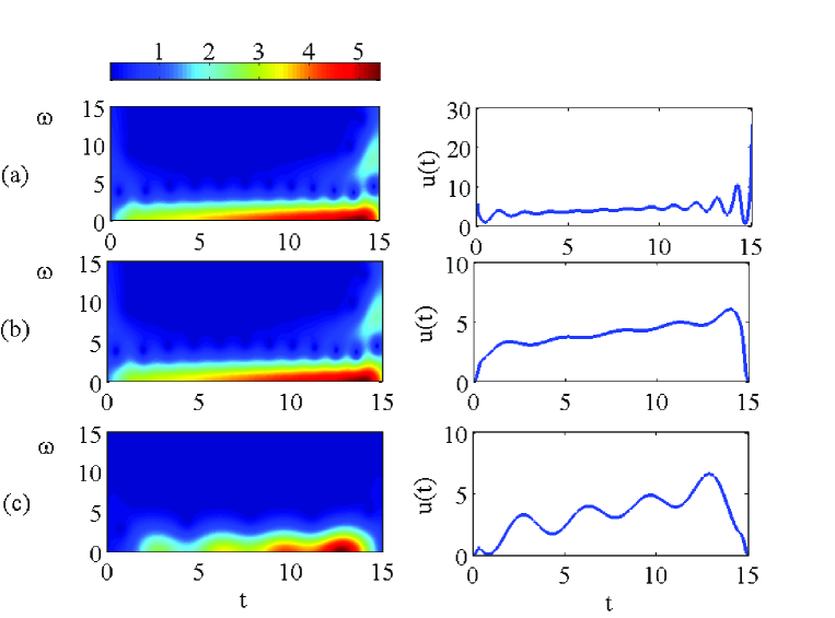
Figure 5: (color online) Windowed Fourier Transform of the control signals (left column) and the time resolved control signals (right column) for a parametrically controlled harmonic oscillator in a thermal reservoir at $k_{\rm B}T=1$. Results in (a) correspond to the optimization in full function space leading to a final-time value $E(\tau)=0.305$. In (b) this control is truncated to a $n=12$-dimensional subspace defined in (14). This control leads to $E(\tau)=0.500$. In (c) results achieved with the PINV method in the same subspace as in (b) are shown producing $E(\tau)=0.323$.

Initially the system is prepared with Gaussian distributed random numbers to satisfy $\mbox{I\negthinspace E}[E(0)]=0.5$. In absence of any control the system would equilibrate to $\mbox{I\negthinspace E}[E]=k_{\rm B}T=1$. The objective here is to further extract energy from the system towards a low energy state

$$\Phi[q(\tau),p(\tau)]=\mbox{I\negthinspace E}\left[\frac{q^{2}(\tau)}{2}+\frac{p^{2}(\tau)}{2}\right].$$ (18)

First we want to search for a control function in full function space, as reference solution to which PINV-based results can be compared. As the numeric cost is very high to do optimal control in a $N=2250$ dimensional function space, in particular as for every iteration step (16) has to be solved for $M=1000$ realizations and averaged, the reference result is computed more efficiently from a Fokker-Planck equation [31], which can be mapped to a system of ordinary differential equations in the case of Gaussian probability densities [32, 33].

The top panel of figure 5 shows an optimized full-space control signal without any constraint obtained using Krotov’s algorithm [11], as well as its windowed-Fourier-transformed [34]. This algorithm is similar to a gradient search near convergence points, but has the advantage of better robustness in its dependence on the initial guess. The resulting control signal is basically a ramp superposed with periodic oscillations. Shortly before the end time these oscillations increase markedly in amplitude, leaving the control signal at a very high value at the final time $\tau=15$. These features of the unconstrained optimization are probably not beneficial in an experimental setting. A detailed discussion of this result is given in [35]. With this control the system has its energy reduced to $E(\tau)=0.305$, well below both its initial and thermal equilibrium values.

We now turn our attention to optimization constrained to a subspace, again defined through the modified Fourier basis (14) with n=12.

The middle panel of figure 5 shows a naive projection of the Fokker-Planck result onto this subspace. In the projected control signal a ramp phase can still be distinguished, but the signal is markedly altered at the beginning and end of the time interval. Notably, the high value at the final time is suppressed. Applying this simple post-optimization projection leads to a poor result, $E(\tau)=0.500$.

The optimization result obtained with the PINV method, see panel (c) in figure 5 is $E(\tau)=0.323$, a result only slightly inferior to that obtained with the complex signal shown in (a). The shape of the control pulse found with the PINV method is clearly different to the Fokker-Planck result; the ramp is now superposed with highly developed oscillations. Different control signals yielding comparable values for the optimization objective are not unusual when a simple system is controlled for an extended period of time.

When using a gradient method, there is no guarantee that the minimum it finds is a global one. A good initial guess for the control function can improve the end result significantly. Starting near a minimum also reduces the required number of optimization iterations. Here we use the post-truncated Fokker-Planck result (b) as initial guess. The result shown in (c) is obtained by subsequently applying the PINV version of a steepest descent algorithm with convergence tolerance $\epsilon=10^{-5}$.

As in the deterministic case, we see that the PINV method has significant advantages over a simple projection of a control signal obtained in the unconstrained function space. Although the number of independent variables is drastically reduced in the PINV approach, optimization results of a quality similar to the unconstrained case are obtained.

3.3 Performance considerations

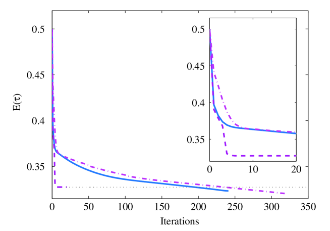
Figure 6: (color online) Comparison of convergence behaviour for PINV-projected time-domain gradient search (solid blue line) and gradient search in coefficient space (dashed purple line). The latter ends prematurely in a plateau (see section 3.3 for details). This problem is absent if coefficients of an orthonormal basis are considered (dash-dotted magenta line). In this case, the iteration progresses in a manner similar to the time-domain case.

All results presented so far were obtained using our projection algorithm in the time domain. An alternative to this approach [1] is optimization based on gradients of the objective with respect to the expansion coefficients $c_{l}$, which involves the matrix $B$ as a Jacobian, $\nabla_{c}J=B\,\nabla_{u}J$. This approach has an equivalent representation in the time domain. It effectively uses the same algorithmic sequence outlined in section 2, with one notable change: The projector $B^{+}B$ is replaced by the matrix $B^{t}B$, which differs from the projector unless an orthonormal basis is chosen.

Figure 6 shows a comparison of the two approaches for the dissipative oscillator discussed in the previous subsection. The solid line (blue) indicates iterations leading to the result shown in figure 5(c). The dashed line (purple) indicates optimization with the alternative approach of directly using the coefficient vector. After significant gains for a few iterations, a plateau is reached; the last iterations shown change the objective only by about $10^{-6}$. After 20 iterations, standard line searches fail (the dotted line is continued as a guide to the eye).

This failure seems remarkable since the control landscapes are the same for both approaches, up to a linear transform mediated by the matrix $B^{t}$. We believe the discrepancy between the two approaches is likely associated with the observation that the linear map described by $B^{t}B$ is highly anisotropic; the non-zero singular values of $B$ differ by many orders of magnitude. The observed behaviour is probably due to rapid convergence along the “easy axes” defined by the anisotropy, followed by extremely slow convergence along the “hard axes”.

This interpretation is supported by the following observation: Using the reduced singular value decomposition [36] of the basis matrix $B=USV^{t}$, it is possible to find an orthonormal basis of the subspace through the column vectors of $V$. With $V^{t}$ substituted for the matrix $B$, there is no anisotropy; $VV^{t}$ is identical to the projector as $B^{+}B$. An optimization using coefficients for the orthogonal basis (dash-dotted, magenta) now shows behaviour similar to the time-domain optimization.

4 Conclusion and discussion

We have developed a method to adapt standard, gradient-based techniques to the problem of experimentally realizable control functions which are characterized by a function space of finite, typically small dimension. This reduced space is defined as the span of an arbitrary set of functions. Despite this generality, the projection of arbitrary functions to the reduced space as well as transformation between a vector of function values over a discretized time axis and a coordinate vector in the reduced space can be easily accomplished by using the Moore-Penrose pseudoinverse.

It is imperative that the iterative computation of optimal control solutions be performed entirely in the control subspace of interest. Imposing a single projection on a control solution computed without constraints yields unacceptable results. It is therefore of great importance that the transformations and projections implicit in each iteration step are efficiently computed; this is the case for the Moore-Penrose pseudoinverse.

The reduced dimensionality of the function space to be searched typically reduces the numerical cost of optimization, in particular when using quasi-Newton methods. In addition, we note arbitrary parametrizations of admissible control fields may introduce artificial anisotropies to the control problem, potentially leading to a serious slowdown of gradient methods.

When using projections in the time domain, on the other hand, fairly rapid convergence can be seen. Similar observations can be made in the case of parameters which are coordinates of an orthonormal basis. Iterations already close to an extremum can be accelerated by using quasi-Newton methods like BFGS, a particular advantage when high-precision solutions are required, as, e.g., in the context of quantum information processing.

Our method is easily generalized to non-linear parameterizations of admissible control functions. In this case, the sets of admissible control functions are manifolds rather than linear spaces. However, the present approach can be adapted by computing the projected gradient in the tangent space at the current iteration point and using the natural mapping from the parameter space to the manifold.

The class of algorithms studied here may find applications beyond optimal control theory. Dynamic programming can be thought of as a formal analogue of optimal control theory, with time replaced by an arbitrary parameter of a recursion relation formally analogous to an equation of motion. This opens up the prospect of interdisciplinary applications or applications outside physics, e.g., problems in economics.

References

References

- [1] Thomas E. Skinner and Naum I. Gershenzon. Optimal control design of pulse shapes as analytic functions. Journal of Magnetic Resonance, 204(2):248 – 255, 2010.
- [2] Katharine W. Moore and Herschel Rabitz. Exploring constrained quantum control landscapes. The Journal of Chemical Physics, 137(134113), 2012.
- [3] Jr. A. Bryson and Y.-C. Ho. Applied optimal control. Hemisphere, Washington, D.C., 1975.
- [4] Jon H. Davis. Foundations of Deterministic and Stochastic Control. Birkhäuser Boston, 2002.
- [5] Constantin Brif, Raj Charkrabarti, and Herschel Rabitz. Control of quantum phenomena: past, present and future. New Journal of Physics, 12:075008, 2010.
- [6] Steffen J. Glaser, T. Schulte-Herbrüggen, M. Sieveking, O. Schedletzky, N.C. Nielsen, O.W. Sørensen, and C. Griesinger. Unitary Control in Quantum Ensembles: Maximizing Signal Intensity in Coherent Spectroscopy. Science, 280:421, 1998.
- [7] Shlomo E. Sklarz and David J. Tannor. Loading a Bose-Einstein condensate onto a optical lattice: An application of optimal control theory to the nonlinear Schrödinger equation. Physical Review A, 66:053619, 2002.
- [8] J. P. Palao and R. Kosloff. Quantum computing by an optimal control algorithm for unitary transformations. Phys. Rev. Lett., 89:188301, 2002.
- [9] T. Calarco, E. A. Hinds, D. Jaksch, J. Schmiedmayer, J. I. Cirac, and P. Zoller. Quantum gates with neutral atoms: Controlling collisional interactions in time-dependent traps. Phys. Rev. A, 61:022304, 2000.
- [10] Rebecca Schmidt, Jürgen T. Stockburger, and Joachim Ankerhold. Almost local generation of Einstein-Podolsky-Rosen entanglement in nonequilibrium open systems. Phys. Rev. A, 88:052321, Nov 2013.
- [11] V.F. Krotov. Global Methods in Optimal Control Theory. Pure and applied mathematics. Marcel Dekker, New York, 1996.
- [12] Navin Khaneja, Timo Reiss, Cindie Kehlet, Thomas Schulte-Herbrüggen, and Steffen J. Glaser. Optimal control of coupled spin dynamics: design of NMR pulse sequences by gradient ascent algorithms. Journal of Magnetic Resonance, 172(2):296 – 305, 2005.
- [13] Thomas Stefan Häberle and Matthias Freyberger. Entangled particles in a dynamically controlled trap. Phys. Rev. A, 89:052332, May 2014.
- [14] Michael H Goerz, Daniel M Reich, and Christiane P Koch. Optimal control theory for a unitary operation under dissipative evolution. New Journal of Physics, 16(5):055012, 2014.
- [15] P. de Fouquieres, S.G. Schirmer, S.J. Glaser, and Ilya Kuprov. Second order gradient ascent pulse engineering. Journal of Magnetic Resonance, 212(2):412 – 417, 2011.
- [16] T. Caneva, T. Calarco, and S. Montangero. Chopped random-basis quantum optimization. Phys. Rev. A, 84:022326, 2011.
- [17] Lyndon Emsley and Geoffrey Bodenhausen. Gaussian pulse cascades: New analytical functions for rectangular selective inversion and in-phase excitation in NMR. Chemical Physics Letters, 165(6):469 – 476, 1990.
- [18] Björn Bartels and Florian Mintert. Smooth optimal control with floquet theory. Phys. Rev. A, 88:052315, Nov 2013.
- [19] Oriol Romero-Isart and Juan José García-Ripoll. Quantum ratchets for quantum communication with optical superlattices. Phys. Rev. A, 76:052304, Nov 2007.
- [20] Patrick Doria, Tommaso Calarco, and Simone Montangero. Optimal control technique for many-body quantum dynamics. Phys. Rev. Lett., 106:190501, May 2011.
- [21] Albert Verdeny, Łukasz Rudnicki, Cord A. Müller, and Florian Mintert. Optimal control of effective hamiltonians. Phys. Rev. Lett., 113:010501, Jul 2014.
- [22] K. Graichen and N. Petit. Incorporating a class of constraints into the dynamics of optimal control problems. Optimal Control Applications and Methods, 30(6):537–561, 2009.
- [23] Knut Graichen, Andreas Kugi, Nicolas Petit, and Francois Chaplais. Handling constraints in optimal control with saturation functions and system extension. Systems & Control Letters, 59(11):671 – 679, 2010.
- [24] Ido Schaefer and Ronnie Kosloff. Optimal-control theory of harmonic generation. Phys. Rev. A, 86:063417, Dec 2012.
- [25] D. Sugny, S. Vranckx, M. Ndong, O. Atabek, and M. Desouter-Lecomte. External constraints on optimal control strategies in molecular orientation and photofragmentation: role of zero-area fields. Journal of Modern Optics, 61(10):816–821, 2014.
- [26] José P. Palao, Daniel M. Reich, and Christiane P. Koch. Steering the optimization pathway in the control landscape using constraints. Phys. Rev. A, 88:053409, Nov 2013.
- [27] R. Penrose. A generalized inverse for matrices. Proceedings of the Cambridge Philosophical Society, 51:406–413, 1955.
- [28] S. Boyd and L. Vandenberghe. Convex Optimization. Cambridge University Press, Cambridge, 2004.
- [29] R. Fletcher. Practical methods in optimization. Wiley, 2 edition, 1987.
- [30] Jorge Nocedal and Stephen J. Wright. Numerical optimization. Springer, New York, NY, 2. ed. edition, 2006.
- [31] Hannes Risken. The Fokker-Planck equation: methods of solution and applications. Springer, Berlin, Heidelberg, New York, 2 edition, 1996.
- [32] R. Schmidt, A. Negretti, J. Ankerhold, T. Calarco, and J. T. Stockburger. Optimal control of open quantum systems: Cooperative effects of driving and dissipation. Phys. Rev. Lett., 107:130404, Sep 2011.
- [33] Jürgen T. Stockburger, Rebecca Schmidt, and Joachim Ankerhold. Entanglement generation through local field and quantum dissipation. arXiv:1404.7686 [quant-ph], 2014.
- [34] J.B. Allen. Short term spectral analysis, synthesis, and modification by discrete fourier transform. Acoustics, Speech and Signal Processing, IEEE Transactions on, 25(3):235–238, Jun 1977.
- [35] R. Schmidt, S. Rohrer, J. Ankerhold, and J. T. Stockburger. Cooling of quantum systems through optimal control and dissipation. Physica Scripta, 2012(T151):014034, 2012.
- [36] Lloyd N. Trefethen and David Bau. Numerical linear algebra. Society for Industrial and Applied Mathematics, Philadelphia, 1997.