Convolution based smooth approximations to the absolute value function with application to non-smooth regularization

Abstract

We present new convolution based smooth approximations to the absolute value function and apply them to construct gradient based algorithms such as the nonlinear conjugate gradient scheme to obtain sparse, regularized solutions of linear systems $Ax=b$, a problem often tackled via iterative algorithms which attack the corresponding non-smooth minimization problem directly. In contrast, the approximations we propose allow us to replace the generalized non-smooth sparsity inducing functional by a smooth approximation of which we can readily compute gradients and Hessians. The resulting gradient based algorithms often yield a good estimate for the sought solution in few iterations and can either be used directly or to quickly warm start existing algorithms.

1 Introduction

Consider the linear system $Ax=b$, where $A\in\mathbb{R}^{m\times n}$ and $b\in\mathbb{R}^{m}$. Often, in linear systems arising from physical inverse problems, we have more unknowns than data: $m\ll n$ [21] and the right hand side of the system which we are given contains noise. In such a setting, it is common to introduce a constraint on the solution, both to account for the possible ill-conditioning of $A$ and noise in $b$ (regularization) and for the lack of data with respect to the number of unknown variables in the linear system. A commonly used constraint is sparsity: to require the solution $x$ to have few nonzero elements compared to the dimension of $x$. A common way of finding a sparse solution to the under-determined linear system $Ax=b$ is to solve the classical Lasso problem [9]. That is, to find $\bar{x}=\arg\min_{x}F_{1}(x)$ where

$$F_{1}(x)=\|Ax-b\|_{2}^{2}+2\tau\|x\|_{1},$$

i.e., the least squares problem with an $\ell_{1}$ regularizer, governed by the regularization parameter $\tau>0$ [7]. For any $p\geq 1$, the map $\|x\|_{p}:=\left(\sum_{k=1}^{n}|x_{k}|^{p}\right)^{\frac{1}{p}}$ (for any $x\in\mathbb{R}^{n}$) is called the $\ell_{p}$-norm on $\mathbb{R}^{n}$. For $p=1$, the $||\cdot||_{1}$ norm is called an $\ell_{1}$ norm and is convex. Besides $F_{1}(x)$, we also consider the more general $\ell_{p}$ functional (for $p>0$) of which $\ell_{1}$ is a special case:

$$F_{p}(x)=||Ax-b||_{2}^{2}+2\tau\left(\sum_{k=1}^{n}|x_{k}|^{p}\right)^{\frac{1}{p}},$$ (1.1)

As $p\to 0$, the right term of this functional approximates the count of nonzeros or the so called $\ell_{0}$ “norm” (which is not a proper norm):

$$||x||_{0}=\lim_{p\to 0}\|x\|_{p}=\lim_{p\to 0}\left(\sum_{k=1}^{n}|x_{k}|^{p}\right)^{1/p},$$

which can be seen from Figure 1.

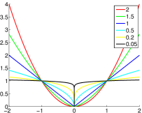
Figure 1: $|x|^{p}$ plotted for different values of $p$, as $p\to 0$, the plot approaches an indicator function.

For $0<p<1$, (1.1) is not convex. However, the minimization of non-smooth non-convex functions has been shown to produce good results in some compressive sensing applications [4]. The non-smoothness of the functional $F_{p}(x)$, however, complicates its minimization from an algorithmic point of view. The non-smooth part of (1.1) is due to the absolute value function $g(x_{k})=|x_{k}|$. Because the gradient of $F_{p}(x)$ cannot be obtained, different minimization techniques such as sub-gradient methods are usually used [19]. For the convex $p=1$ case, various thresholding based methods have become popular. A particularly successful example is the soft thresholding based method FISTA [2]. This algorithm is an accelerated version of a soft thresholded Landweber iteration [12]:

$$x^{n+1}=\mathbb{S}_{\tau}(x^{n}+A^{T}b-A^{T}Ax^{n})$$ (1.2)

The soft thresholding function $\mathbb{S}_{\tau}:\mathbb{R}^{n}\to\mathbb{R}^{n}$ [7] is defined by

$$\left(\mathbb{S}_{\tau}(x)\right)_{k}=\operatorname{sgn}(x_{k})\max{\{0,|x_{k}|-\tau\}},\ \forall\,k=1,\ldots,n,\ \forall\,x\in\mathbb{R}^{n}.$$

The scheme (1.2) is known to converge from some initial guess, but slowly, to the $\ell_{1}$ minimizer [7]. The thresholding in (1.2) is performed on $x^{n}-\nabla_{x}(\frac{1}{2}||Ax^{n}-b||_{2}^{2})=x^{n}-A^{T}(Ax^{n}-b)$, which is a very simple gradient based scheme with a constant line search [10]. Naturally, more advanced gradient schemes may be able to provide better numerical performance; however, they are possible to utilize only if we are able to compute the gradient of the functional we want to minimize.

In this article, we present new smooth approximations to the non-smooth absolute value function $g(t)=|t|$, computed via convolution with a Gaussian function. This allows us to replace the non-smooth objective function $F_{p}(x)$ by a smooth functional $H_{p,\sigma}(x)$, which is close to $F_{p}(x)$ in value (as the parameter $\sigma\to 0$). Since the approximating functional $H_{p,\sigma}(x)$ is smooth, we can compute its gradient vector $\nabla_{x}H_{p,\sigma}(x)$ and Hessian matrix $\nabla^{2}_{x}H_{p,\sigma}(x)$. We are then able to use gradient based algorithms such as conjugate gradients to approximately minimize $F_{p}(x)$ by working with the approximate functional and gradient pair. The resulting gradient based methods we show are simple to implement and in many instances yield good numerical performance in few iterations.

We remark that this article is not the first in attempting to use smooth approximations for sparsity constrained problems. A smooth $\ell_{0}$ norm approach has been proposed in [14]. In this article, we propose a more general method which can be used for $F_{p}(x)$, including the popular $\ell_{1}$ case. The absolute value function which appears in non-smooth regularization is just one application of the convolution based smoothing approach we introduce here, which can likely be extended to different non-smooth functions.

2 Smooth approximation of absolute value function

2.1 Some existing smoothing techniques

One simple smooth approximation to the absolute value function is given by $s_{\sigma}(t)=\sqrt{t^{2}+\sigma^{2}}$ with $\sigma>0\in\mathbb{R}$.

Lemma 2.1

The approximation $s_{\sigma}(t)$ to $|t|$ satisfies:

$$\frac{\mathrm{d}}{\mathrm{d}t}s_{\sigma}(t)=t\left(t^{2}+\sigma^{2}\right)^{-\frac{1}{2}}$$ (2.1)

and

$$\left||t|-s_{\sigma}(t)\right|\leq\sigma$$ (2.2)

• To establish (2.2), consider the inequality:

  $$\frac{t^{2}}{\sqrt{t^{2}+\sigma^{2}}}\leq|t|\leq\sqrt{t^{2}+\sigma^{2}}$$

  It follows that:

  $$\left||t|-s_{\sigma}(t)\right|\leq\sqrt{t^{2}+\sigma^{2}}-\frac{t^{2}}{\sqrt{t^{2}+\sigma^{2}}}=\frac{\sigma^{2}}{\sqrt{t^{2}+\sigma^{2}}}\leq\sigma$$

  $\Box$

Another well known smoothing technique for the absolute value is the so called Huber function [3].

Lemma 2.2

The Huber function defined as:

$$p_{\sigma}(t)=\left\{\begin{array}[]{ll}\frac{t^{2}}{2\sigma}&\mbox{, }|t|\leq\sigma\\ |t|-\frac{\sigma}{2}&\mbox{, }|t|\geq\sigma\end{array}\right.$$ (2.3)

corresponds to the minimum value of the function

$$\min_{x\in\mathbb{R}}\left\{\frac{1}{2\sigma}(x-t)^{2}+|x|\right\}$$ (2.4)

It follows that:

$$\frac{\mathrm{d}}{\mathrm{d}t}p_{\sigma}(t)=\left\{\begin{array}[]{ll}\frac{t}{\sigma}&\mbox{, }|t|\leq\sigma\\ sgn(t)&\mbox{, }|t|\geq\sigma\end{array}\right.$$ (2.5)

and

$$\left||t|-p_{\sigma}(t)\right|\leq\frac{\sigma}{2}$$ (2.6)

• The derivation follows by means of the soft thresholding operator (3.19), which is known to satisfy the relation $\mathbb{S}_{\sigma}(t)=\arg\min_{x}\left\{(x-t)^{2}+2\sigma|x|\right\}$ [7]. When $|t|\leq\sigma$, $\mathbb{S}_{\sigma}(t)=0$. Plugging this into (2.4), we obtain:

  $$\min\left\{\frac{1}{2\sigma}(x-t)^{2}+|x|\right\}=\frac{1}{2\sigma}(0-t)^{2}+|0|=\frac{t^{2}}{2\sigma}$$

  When $|t|>\sigma$, $S_{\sigma}(t)=t-\sigma$ (when $t>\sigma$) or $t+\sigma$ (when $t<-\sigma$). Taking the case $t>\sigma$, we have $|t|=t$, $|t-\sigma|=t-\sigma$ and:

  $$\min\left\{\frac{1}{2\sigma}(x-t)^{2}+|x|\right\}=\frac{1}{2\sigma}(t-\sigma-t)^{2}+|t-\sigma|=\frac{1}{2\sigma}\sigma^{2}+(t-\sigma)=|t|-\frac{\sigma}{2}$$

  Similarly, when $t<-\sigma$, we have $|t|=-t$, $|t+\sigma|=-t-\sigma$ and:

  $$\min\left\{\frac{1}{2\sigma}(x-t)^{2}+|x|\right\}=\frac{1}{2\sigma}(t+\sigma-t)^{2}+|t+\sigma|=\frac{1}{2\sigma}\sigma^{2}-t-\sigma=|t|-\frac{\sigma}{2}$$

  and so we obtain both parts of $\eqref{eq:huber_fcn}$. To show (2.6), consider both cases of $\eqref{eq:huber_fcn}$. When $|t|\geq\sigma$, $\left||t|-p_{\sigma}(t)\right|=\left||t|-|t|-\frac{\sigma}{2}\right|=\frac{\sigma}{2}$. When $|t|\leq\sigma$, we evaluate $\left||t|-\frac{t^{2}}{2\sigma}\right|$. Let $u=|t|$, then for $u\leq\sigma$, $u-\frac{u^{2}}{2\sigma}>0$ and $u-\frac{u^{2}}{2\sigma}=\frac{2\sigma u-u^{2}}{2\sigma}$. Let $r(u)=2\sigma u-u^{2}\implies r^{\prime}(u)=2\sigma-2u=0$ and $r^{\prime\prime}(u)=-2<0$. Hence the max occurs at $u=\sigma$, which gives $\max\left(\frac{2\sigma u-u^{2}}{2\sigma}\right)=\frac{\sigma^{2}}{2\sigma}=\frac{\sigma}{2}$ when $u=|t|\leq\sigma$. $\Box$

Lemmas 2.1 and 2.2 imply that we can approximate the one norm of vector $x\in\mathbb{R}^{n}$ as $\|x\|_{1}\approx\displaystyle\sum_{i=1}^{n}s_{\sigma}(x_{i})$ or as $\|x\|_{1}\approx\displaystyle\sum_{i=1}^{n}p_{\sigma}(x_{i})$. From (2.2) and (2.6), the approximations satisfy:

$$\sum_{k=1}^{n}s_{\sigma}(x_{k})\leq\|x\|_{1}\leq\displaystyle\sum_{k=1}^{n}s_{\sigma}(x_{k})+\sigma n\quad\mbox{and}\quad\displaystyle\sum_{k=1}^{n}p_{\sigma}(x_{k})\leq\|x\|_{1}\leq\displaystyle\sum_{k=1}^{n}p_{\sigma}(x_{k})+\frac{\sigma n}{2}$$

The smooth approximation for $\|x\|_{1}$ allows us to approximate the $\ell_{1}$ functional $F_{1}(x)$ as:

$$S_{1,\sigma}(x)=||Ax-b||_{2}^{2}+2\tau\displaystyle\sum_{k=1}^{n}s_{\sigma}(x_{k})\quad\mbox{and}\quad P_{1,\sigma}(x)=||Ax-b||_{2}^{2}+2\tau\displaystyle\sum_{k=1}^{n}p_{\sigma}(x_{k})$$

Note that from (2.1) and (2.5), the corresponding gradient vectors $\nabla S_{1,\sigma}(x)$ and $\nabla P_{1,\sigma}(x)$ are given by:

$$\nabla S_{1,\sigma}(x)=2A^{T}(Ax-b)+2\tau\left\{s^{\prime}_{\sigma}(x_{k})\right\}_{k=1}^{n}\quad\mbox{and}\quad\nabla P_{1,\sigma}(x)=2A^{T}(Ax-b)+2\tau\left\{p^{\prime}_{\sigma}(x_{k})\right\}_{k=1}^{n}$$

with $s^{\prime}_{\sigma}(x_{k})=x_{k}\left(x_{k}^{2}+\sigma^{2}\right)^{-\frac{1}{2}}$ and $p^{\prime}_{\sigma}(x_{k})=\left\{\begin{array}[]{ll}\frac{x_{k}}{\sigma}&\mbox{, }|x_{k}|\leq\sigma\\ sgn(x_{k})&\mbox{, }|x_{k}|\geq\sigma\end{array}\right.$. The advantage of working with the smooth functionals instead of $F_{1}(x)$ is that given the gradients we can use gradient based methods as we later describe. However, we cannot compute the Hessian matrix of $P_{1,\sigma}(x)$ because $p_{\sigma}(x_{k})$ is not twice differentiable, while $S_{1,\sigma}(x)$ is a less accurate approximation for $F_{1}(x)$. In the next section we introduce a new approximation to the absolute value based on convolution with a Gaussian kernel which addresses both of these concerns.

2.2 Mollifiers and Approximation via Convolution

In mathematical analysis, the concept of mollifiers is well known. Below, we state the definition and convergence result regarding mollifiers, as exhibited in [8]. A smooth function $\psi_{\sigma}:\mathbb{R}\to\mathbb{R}$ is said to be a (non-negative) mollifier if it has finite support, is non-negative $(\psi\geq 0)$, and has area $\int_{\mathbb{R}}\psi(t)\mathrm{d}t=1$. For any mollifier $\psi$ and any $\sigma>0$, define the parametric function $\psi_{\sigma}:\mathbb{R}\to\mathbb{R}$ by: $\psi_{\sigma}(t):=\frac{1}{\sigma}\psi\left(\frac{t}{\sigma}\right)$, for all $t\in\mathbb{R}$. Then $\{\psi_{\sigma}:\sigma>0\}$ is a family of mollifiers, whose support decreases as $\sigma\to 0$, but the volume under the graph always remains equal to one. We then have the following important lemma for the approximation of functions, whose proof is given in [8].

Lemma 2.3

For any continuous function $g\in L^{1}(\Theta)$ with compact support and $\Theta\subseteq\mathbb{R}$, and any mollifier $\psi:\mathbb{R}\to\mathbb{R}$, the convolution $\psi_{\sigma}*g$, which is the function defined by:

$$(\psi_{\sigma}*g)(t):=\int_{\mathbb{R}}\psi_{\sigma}(t-s)g(s)\mathrm{d}s=\int_{\mathbb{R}}\psi_{\sigma}(s)g(t-s)\mathrm{d}s,\ \forall\,t\in\mathbb{R},$$

converges uniformly to $g$ on $\Theta$, as $\sigma\to 0$.

Inspired by the above results, we will now use convolution with approximate mollifiers to approximate the absolute value function $g(t)=|t|$ (which is not in $L^{1}(\mathbb{R})$) with a smooth function. We start with the Gaussian function $K(t)=\frac{1}{\sqrt{2\pi}}\exp\left(-\frac{t^{2}}{2}\right)$ (for all $t\in\mathbb{R}$), and introduce the $\sigma$-dependent family:

$$K_{\sigma}(t):=\frac{1}{\sigma}K\left(\frac{t}{\sigma}\right)=\frac{1}{\sqrt{2\pi\sigma^{2}}}\exp\left(-\frac{t^{2}}{2\sigma^{2}}\right),\quad\forall\,t\in\mathbb{R}.$$ (2.7)

This function is not a mollifier because it does not have finite support. However, this function is coercive, that is, for any $\sigma>0$, $K_{\sigma}(t)\to 0$ as $|t|\to\infty$. In addition, we have that $\int_{-\infty}^{\infty}K_{\sigma}(t)\,\mathrm{d}t=1$ for all $\sigma>0$:

$$\int_{-\infty}^{\infty}\!K_{\sigma}(t)\,\mathrm{d}t = \frac{1}{\sqrt{2\pi\sigma^{2}}}\int_{\mathbb{R}}\exp\left(-\frac{t^{2}}{2\sigma^{2}}\right)\,\mathrm{d}t=\frac{2}{\sqrt{2\pi\sigma^{2}}}\int_{0}^{\infty}\exp\left(-\frac{t^{2}}{2\sigma^{2}}\right)\,\mathrm{d}t$$

$$= \frac{2}{\sqrt{2\pi\sigma^{2}}}\int_{0}^{\infty}\exp(-u^{2})\sqrt{2}\sigma\,\mathrm{d}u=\frac{2}{\sqrt{2\pi\sigma^{2}}}\sqrt{2}\sigma\frac{\sqrt{\pi}}{2}=1.$$

Figure 2 below presents a plot of the function $K_{\sigma}$ in relation to the particular choice $\sigma=0.01$. We see that $K_{\sigma}(t)\geq 0$ and $K_{\sigma}(t)$ is very close to zero for $|t|>4\sigma$. In this sense, the function $K_{\sigma}$ is an approximate mollifier.

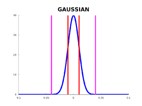
Figure 2: $K_{\sigma}(t)$ and vertical lines at $(-\sigma,\sigma)$ and $(-4\sigma,4\sigma)$ for $\sigma=0.01$.

Let us now compute the limit $\lim_{\sigma\to 0}K_{\sigma}(t)$. For $t=0$, it is immediate that $\lim_{\sigma\to 0}K_{\sigma}(0)=\infty$. For $t\neq 0$, we use l’Hôspital’s rule:

$$\lim_{\sigma\to 0}K_{\sigma}(t)=\lim_{\sigma\to 0}\frac{1}{\sqrt{2\pi\sigma^{2}}}\exp\left(-\frac{t^{2}}{2\sigma^{2}}\right)=\lim_{\gamma\to\infty}\frac{\gamma}{\sqrt{2\pi}\exp\left(\frac{\gamma^{2}t^{2}}{2}\right)}=\frac{1}{\sqrt{2\pi}}\lim_{\gamma\to\infty}\frac{1}{\gamma\,t^{2}\exp\left(\frac{\gamma^{2}t^{2}}{2}\right)}=0,$$

with $\gamma=\frac{1}{\sigma}$. We see that $K_{\sigma}(t)$ behaves like a Dirac delta function $\delta_{0}(x)$ with unit integral over $\mathbb{R}$ and the same pointwise limit. Thus, for small $\sigma>0$, we expect that the absolute value function can be approximated by its convolution with $K_{\sigma}$, i.e.,

$$|t|\approx\phi_{\sigma}(t),\quad\forall\,t\in\mathbb{R},$$ (2.8)

where the function $\phi_{\sigma}:\mathbb{R}\to\mathbb{R}$ is defined as the convolution of $K_{\sigma}$ with the absolute value function:

$$\phi_{\sigma}(t):=(K_{\sigma}*|\cdot|)(t)=\frac{1}{\sqrt{2\pi\sigma^{2}}}\int_{-\infty}^{\infty}|t-s|\exp\left(-\frac{s^{2}}{2\sigma^{2}}\right)\mathrm{d}s,\quad\forall\,t\in\mathbb{R}.$$ (2.9)

We show in Proposition 2.6 below, that the approximation in (2.8) converges in the $L^{1}$ norm (as $\sigma\to 0$). The advantage of using this approximation is that $\phi_{\sigma}$, unlike the absolute value function, is a smooth function.

Before we state the convergence result in Proposition 2.6, we express the convolution integral and its derivative in terms of the well-known error function [1].

Lemma 2.4

For any $\sigma>0$, define $\phi_{\sigma}:\mathbb{R}\to\mathbb{R}$ as in (2.9) Then we have that for all $t\in\mathbb{R}$:

$$\phi_{\sigma}(t)\,= \ t\operatorname{erf}\left(\frac{t}{\sqrt{2}\sigma}\right)+\sqrt{\frac{2}{\pi}}\sigma\exp\left(-\frac{t^{2}}{2\sigma^{2}}\right),$$ (2.10)

$$\frac{\mathrm{d}}{\mathrm{d}t}\,\phi_{\sigma}(t)\,= \ \operatorname{erf}\left(\frac{t}{\sqrt{2}\sigma}\right),$$ (2.11)

where the error function is defined as:

$$\operatorname{erf}(t)=\frac{2}{\sqrt{\pi}}\int_{0}^{t}\exp(-u^{2})\mathrm{d}u\quad\forall\,t\in\mathbb{R}.$$

• Fix $\sigma>0$. Define $C_{\sigma}:\mathbb{R}_{+}\times\mathbb{R}$ by

  $$C_{\sigma}(T,t) := \int_{-T}^{T}|t-s|K_{\sigma}(s)\mathrm{d}s=\frac{1}{\sqrt{2\pi\sigma^{2}}}\int_{-T}^{T}|t-s|\exp\left(-\frac{s^{2}}{2\sigma^{2}}\right)\mathrm{d}s,\quad\forall\,t\in\mathbb{R},\ T\geq 0.$$

  We can remove the absolute value sign in the integration above by breaking up the integral into intervals from $-T$ to $t$ and from $t$ to $T$ where $|t-s|$ can be replaced by $(t-s)$ and $(s-t)$, respectively. Expanding the above we have that:

  $$\sqrt{2\pi\sigma^{2}}C_{\sigma}(T,t) = \int_{-T}^{T}|t-s|\exp\left(-\frac{s^{2}}{2\sigma^{2}}\right)\mathrm{d}s$$

  $$= \int_{-T}^{t}(t-s)\exp\left(-\frac{s^{2}}{2\sigma^{2}}\right)\mathrm{d}s+\int_{t}^{T}(s-t)\exp\left(-\frac{s^{2}}{2\sigma^{2}}\right)\mathrm{d}s$$

  $$= t\left(\int_{-T}^{t}\exp\left(-\frac{s^{2}}{2\sigma^{2}}\right)\mathrm{d}s-\int_{t}^{T}\exp\left(-\frac{s^{2}}{2\sigma^{2}}\right)\mathrm{d}s\right)$$

  $$\qquad+\int_{-T}^{t}\exp\left(-\frac{s^{2}}{2\sigma^{2}}\right)(-s)\mathrm{d}s+\int_{t}^{T}\exp\left(-\frac{s^{2}}{2\sigma^{2}}\right)s\,\mathrm{d}s$$

  $$= \sqrt{2}\sigma t\left(\int_{-T/\sqrt{2}\sigma}^{t/\sqrt{2}\sigma}\exp\left(-u^{2}\right)\mathrm{d}u-\int_{t/\sqrt{2}\sigma}^{T/\sqrt{2}\sigma}\exp\left(-u^{2}\right)\mathrm{d}u\right)$$

  $$\qquad+\sigma^{2}\left(\int_{-T}^{t}\exp\left(-\frac{s^{2}}{2\sigma^{2}}\right)\left(-\frac{s}{\sigma^{2}}\right)\mathrm{d}s-\int_{t}^{T}\exp\left(-\frac{s^{2}}{2\sigma^{2}}\right)\left(-\frac{s}{\sigma^{2}}\right)\mathrm{d}s\right).$$

  Next, making use of the definition of the error function, the fact that it’s an odd function (i.e. $\operatorname{erf}(-t)=-\operatorname{erf}(t)$), and of the fundamental theorem of calculus, we have:

  $$\sqrt{2\pi\sigma^{2}}C_{\sigma}(T,t) = \sqrt{\frac{\pi}{2}}\sigma t\left(\operatorname{erf}\left(\frac{t}{\sqrt{2}\sigma}\right)-\operatorname{erf}\left(\frac{-T}{\sqrt{2}\sigma}\right)-\operatorname{erf}\left(\frac{T}{\sqrt{2}\sigma}\right)+\operatorname{erf}\left(\frac{t}{\sqrt{2}\sigma}\right)\right)$$

  $$\qquad+\sigma^{2}\left(\int_{-T}^{t}\frac{\mathrm{d}}{\mathrm{d}s}\left(\exp\left(-\frac{s^{2}}{2\sigma^{2}}\right)\right)\mathrm{d}s-\int_{t}^{T}\frac{\mathrm{d}}{\mathrm{d}s}\left(\exp\left(-\frac{s^{2}}{2\sigma^{2}}\right)\right)\mathrm{d}s\right)$$

  $$= \sqrt{2\pi}\sigma t\operatorname{erf}\left(\frac{t}{\sqrt{2}\sigma}\right)+2\sigma^{2}\left(\exp\left(-\frac{t^{2}}{2\sigma^{2}}\right)-\exp\left(-\frac{T^{2}}{2\sigma^{2}}\right)\right).$$

  Since $\exp\left(-\frac{T^{2}}{2\sigma^{2}}\right)\to 0$ as $T\to\infty$, we have:

  $$\phi_{\sigma}(t)\,=\,(K_{\sigma}*|\cdot|)(t) = \lim_{T\to\infty}C_{\sigma}(T,t)=\frac{1}{\sqrt{2\pi}\sigma}\sqrt{2\pi}\sigma t\operatorname{erf}\left(\frac{t}{\sqrt{2}\sigma}\right)+\frac{2}{\sqrt{2\pi}\sigma}\sigma^{2}\exp\left(-\frac{t^{2}}{2\sigma^{2}}\right)$$

  $$= t\operatorname{erf}\left(\frac{t}{\sqrt{2}\sigma}\right)+\sqrt{\frac{2}{\pi}}\sigma\exp\left(-\frac{t^{2}}{2\sigma^{2}}\right).$$

  This proves (2.10). To derive (2.11), we use

  $$\frac{\mathrm{d}}{\mathrm{d}t}\operatorname{erf}\left(\frac{t}{\sqrt{2}\sigma}\right)=\frac{2}{\sqrt{\pi}}\frac{\mathrm{d}}{\mathrm{d}t}\left[\int_{0}^{\left(\frac{t}{\sqrt{2}\sigma}\right)}\exp(-u^{2})\mathrm{d}u\right]=\frac{\sqrt{2}}{\sigma\sqrt{\pi}}\exp\left(-\frac{t^{2}}{2\sigma^{2}}\right),$$ (2.12)

  Plugging in, we get:

  $$\frac{\mathrm{d}}{\mathrm{d}t}\,\phi_{\sigma}(t) = \frac{\mathrm{d}}{\mathrm{d}t}\left(t\operatorname{erf}\left(\frac{t}{\sqrt{2}\sigma}\right)+\sqrt{\frac{2}{\pi}}\sigma\exp\left(-\frac{t^{2}}{2\sigma^{2}}\right)\right)$$

  $$= \operatorname{erf}\left(\frac{t}{\sqrt{2}\sigma}\right)+t\frac{\sqrt{2}}{\sigma\sqrt{\pi}}\exp\left(-\frac{t^{2}}{2\sigma^{2}}\right)-\sqrt{\frac{2}{\pi}}\sigma\frac{2t}{2\sigma^{2}}\exp\left(-\frac{t^{2}}{2\sigma^{2}}\right)$$

  $$= \operatorname{erf}\left(\frac{t}{\sqrt{2}\sigma}\right).$$

  so that (2.11) holds. $\Box$

Next, we review some basic properties of the error function $\operatorname{erf}(t)=\frac{2}{\sqrt{\pi}}\int_{0}^{t}\exp(-s^{2})\mathrm{d}s$ and the Gaussian integral [1]. It is well known that the Gaussian integral satisfies:

$$\int_{-\infty}^{\infty}\exp(-s^{2})\mathrm{d}s=2\int_{0}^{\infty}\exp(-s^{2})\mathrm{d}s=\sqrt{\pi},$$

and, in particular, $0<\operatorname{erf}(t)<1$ for all $t>0$. Using results from [6] on the Gaussian integral, we also have the following bounds for the error function:

Lemma 2.5

The error function $\operatorname{erf}(t)=\frac{2}{\sqrt{\pi}}\int_{0}^{t}\exp(-s^{2})\mathrm{d}s$ satisfies the bounds:

$$\bigl{(}1-\exp(-t^{2})\bigr{)}^{\frac{1}{2}}\leq\operatorname{erf}(t)\leq\bigl{(}1-\exp(-2t^{2})\bigr{)}^{\frac{1}{2}},\quad\forall\,t\geq 0.$$ (2.13)

• In [6], it is shown that for the function $v(t):=\frac{1}{\sqrt{2\pi}}\int_{0}^{t}\exp\left(-\frac{s^{2}}{2}\right)\mathrm{d}s$, the following bounds hold:

  $$\frac{1}{2}\left(1-\exp\left(-\frac{t^{2}}{2}\right)\right)^{\frac{1}{2}}\leq v(t)\leq\frac{1}{2}\left(1-\exp\left(-t^{2}\right)\right)^{\frac{1}{2}},\quad\forall\,t\geq 0.$$ (2.14)

  Now we relate $v(t)$ to the error function. Using the substitution $u=\frac{s}{\sqrt{2}}$:

  $$v(t)=\frac{1}{\sqrt{2\pi}}\int_{0}^{\frac{t}{\sqrt{2}}}\exp(-u^{2})\sqrt{2}\mathrm{d}u=\frac{1}{2}\operatorname{erf}\left(\frac{t}{\sqrt{2}}\right).$$

  From (2.14), it follows that:

  $$\left(1-\exp\left(-\frac{t^{2}}{2}\right)\right)^{\frac{1}{2}}\leq\operatorname{erf}\left(\frac{t}{\sqrt{2}}\right)\leq\left(1-\exp(-t^{2})\right)^{\frac{1}{2}}.$$

  With the substitution $s=\frac{t}{\sqrt{2}}$, we obtain (2.13). $\Box$

Using the above properties of the error function and the Gaussian integral, we can prove our convergence result.

Proposition 2.6

Let $g(t):=|t|$ for all $t\in\mathbb{R}$, and let the function $\phi_{\sigma}:=K_{\sigma}*g$ be defined as in (2.9), for all $\sigma>0$. Then:

$$\lim_{\sigma\to 0}\left\|\phi_{\sigma}-g\right\|_{L^{1}}=0.$$

• By definition of $\phi_{\sigma}$,

  $$\left\|\phi_{\sigma}-g\right\|_{L^{1}}=\int_{-\infty}^{\infty}\bigl{|}(K_{\sigma}*|\cdot|)(t)-|t|\,\bigr{|}\mathrm{d}t=2\int_{0}^{\infty}\bigl{|}(K_{\sigma}*|\cdot|)(t)-t\bigr{|}\mathrm{d}t,$$

  where the last equality follows from the fact that $\phi_{\sigma}-g$ is an even function since both $\phi_{\sigma}$ and $g$ are even functions. Plugging in (2.8), we have:

  $$||\phi_{\sigma}-g||_{L^{1}} = 2\int_{0}^{\infty}\left|t\left(\operatorname{erf}\left(\frac{t}{\sqrt{2}\sigma}\right)-1\right)+\sqrt{\frac{2}{\pi}}\sigma\exp\left(-\frac{t^{2}}{2\sigma^{2}}\right)\right|\mathrm{d}t$$

  $$\leq 2\int_{0}^{\infty}\left|t\left(\operatorname{erf}\left(\frac{t}{\sqrt{2}\sigma}\right)-1\right)\right|+\sqrt{\frac{2}{\pi}}\sigma\exp\left(-\frac{t^{2}}{2\sigma^{2}}\right)\mathrm{d}t$$

  $$= 2\int_{0}^{\infty}t\left(1-\operatorname{erf}\left(\frac{t}{\sqrt{2}\sigma}\right)\right)+\sqrt{\frac{2}{\pi}}\sigma\exp\left(-\frac{t^{2}}{2\sigma^{2}}\right)\mathrm{d}t,$$

  where we have used the inequality $0<\operatorname{erf}(t)<1$ for $t>0$. Next, we analyze both terms of the integral. First, using (2.13), we have:

  $$\left(1-\exp(-t^{2})\right)^{\frac{1}{2}}\leq\operatorname{erf}(t)\implies 1-\operatorname{erf}(t)\leq 1-\left(1-\exp(-t^{2})\right)^{\frac{1}{2}}\leq\exp\left(-\frac{x^{2}}{2}\right),$$

  where the last inequality follows from the fact that $1-\sqrt{1-\alpha}\leq\sqrt{\alpha}$ for $\alpha\in(0,1)$. It follows that:

  $$\int_{0}^{\infty}t\left(1-\operatorname{erf}\left(\frac{t}{\sqrt{2}\sigma}\right)\right)\mathrm{d}t\leq\int_{0}^{\infty}t\exp\left(-\frac{t^{2}}{4\sigma^{2}}\right)\mathrm{d}t=2\sigma^{2}\int_{0}^{\infty}\exp(-u)\mathrm{d}u=2\sigma^{2},$$

  For the second term,

  $$\sqrt{\frac{2}{\pi}}\sigma\int_{0}^{\infty}\exp\left(-\frac{t^{2}}{2\sigma^{2}}\right)\mathrm{d}t=\sqrt{\frac{2}{\pi}}\sigma\left(\sqrt{2}\sigma\int_{0}^{\infty}\exp(-s^{2})\mathrm{d}s\right)=\frac{2}{\sqrt{\pi}}\sigma^{2}\frac{\sqrt{\pi}}{2}=\sigma^{2}.$$

  Thus:

  $$\lim_{\sigma\to 0}\|\phi_{\sigma}-g\|_{L^{1}}\leq 2\lim_{\sigma\to 0}\left(2\sigma^{2}+\sigma^{2}\right)=0.$$

  Hence we have that $\lim_{\sigma\to 0}\|\phi_{\sigma}-g\|_{L^{1}}=0$. $\Box$

Note that in the above proof, $g=|\cdot|\not\in L^{1}$ (since $g(t)\to\infty$ as $t\to\infty$), but the approximation in the $L^{1}$ norm still holds. It is likely that the convolution approximation converges to $g$ in the $L^{1}$ norm for a variety of non-smooth coercive functions $g$, not just for $g(t)=|t|$.

Note from (2.8) that while the approximation $\phi_{\sigma}(t)=K_{\sigma}*|t|$ is indeed smooth, it is positive on $\mathbb{R}$ and in particular $(K_{\sigma}*|\cdot|)(0)=\sqrt{\frac{2}{\pi}}\sigma>0$, although $(K_{\sigma}*|\cdot|)(0)$ does go to zero as $\sigma\to 0$. To address this, we can use different approximations based on $\phi_{\sigma}(t)$ which are zero at zero. Many different alternatives are possible. We describe here two particular approximations. The first is formed by subtracting the value at $0$:

$$\tilde{\phi}_{\sigma}(t)=\phi_{\sigma}(t)-\phi_{\sigma}(0)\,=\,t\operatorname{erf}\left(\frac{t}{\sqrt{2}\sigma}\right)+\sqrt{\frac{2}{\pi}}\sigma\exp\left(\frac{-t^{2}}{2\sigma^{2}}\right)-\sqrt{\frac{2}{\pi}}\sigma,$$ (2.15)

An alternative is to use $\tilde{\phi^{(2)}}_{\sigma}(t)=\phi_{\sigma}(t)-\sqrt{\frac{2}{\pi}}\sigma\exp\left(-t^{2}\right)$ where the subtracted term decreases in magnitude as $t$ becomes larger and only has much effect for $t$ close to zero. We could also simply drop the second term of $\phi_{\sigma}(t)$ to get:

$$\hat{\phi}_{\sigma}(t)=\phi_{\sigma}(t)-\sqrt{\frac{2}{\pi}}\sigma\exp\left(\frac{-t^{2}}{2\sigma^{2}}\right)\,=\,t\operatorname{erf}\left(\frac{t}{\sqrt{2}\sigma}\right)$$ (2.16)

which is zero when $t=0$.

2.3 Comparsion of different approximations

We now illustrate the different convolution based approximations along with the previously discussed $s_{\sigma}(t)$ and $p_{\sigma}(t)$. In Figure 3, we plot the absolute value function $g(t)=|t|$ and the different approximations $\phi_{\sigma}(t),\tilde{\phi}_{\sigma}(t),\hat{\phi}_{\sigma}(t),s_{\sigma}(t)$, and $p_{\sigma}(t)$ for $\sigma_{1}=3e^{-4}$ (larger value corresponding to a worser approximation) and $\sigma_{2}=e^{-4}$ (smaller value corresponding to a better approximation) for a small range of values $t\in(-4.5e^{-4},4.5e^{-4})$ around $t=0$. We may observe that $\phi_{\sigma}(t)$ smooths out the sharp corner of the absolute value, at the expense of being above zero at $t=0$ for positive $\sigma$. The modified approximations $\tilde{\phi}_{\sigma}(t)$ and $\hat{\phi}_{\sigma}(t)$ are zero at zero. However, $\tilde{\phi}_{\sigma}(t)$ over-approximates $|t|$ for all $t>0$ while $\hat{\phi}_{\sigma}(t)$ does not preserve convexity. The three $\phi$ approximations respectively capture the general characteristics possible to obtain with the described convolution approach. From the figure we may observe that $\phi_{\sigma}(t)$ and $\hat{\phi}_{\sigma}(t)$ remain closer to the absolute value curve than $s_{\sigma}(t)$ and $p_{\sigma}(t)$ as $|t|$ becomes larger. The best approximation appears to be $\hat{\phi}_{\sigma}(t)$, which is close to $|t|$ even for the larger value $\sigma_{1}$ and is twice differentiable.

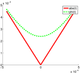
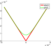
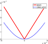
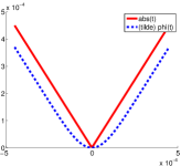
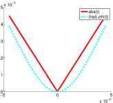
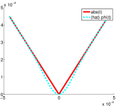
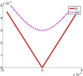
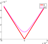
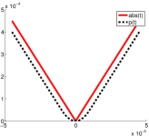
Figure 3: Absolute value function $|t|$ on a fixed interval vs different smooth approximations with $\sigma_{1}=3e^{-4}$ and $\sigma_{2}=e^{-4}$. Row 1: $|t|$ vs $\phi_{\sigma_{1}}(t),\phi_{\sigma_{2}}(t)$. Row 2: $|t|$ vs $\tilde{\phi}_{\sigma_{1}}(t),\tilde{\phi}_{\sigma_{2}}(t)$ and $|t|$ vs $\hat{\phi}_{\sigma_{1}}(t),\hat{\phi}_{\sigma_{2}}(t)$. Row 3: $|t|$ vs $s_{\sigma_{1}}(t),s_{\sigma_{2}}(t)$ and $|t|$ vs $p_{\sigma_{1}}(t),p_{\sigma_{2}}(t)$.

3 Gradient Based Algorithms

In this section, we discuss the use of gradient based optimization algorithms such as steepest descent and conjugate gradients to approximately minimize the functional (1.1):

$$F_{p}(x)=||Ax-b||^{2}_{2}+2\tau\left(\sum_{k=1}^{n}|x_{k}|^{p}\right)^{1/p},$$

where we make use of one of the approximations ($\phi_{\sigma}(x_{k}),\tilde{\phi}_{\sigma}(x_{k}),\hat{\phi}_{\sigma}(x_{k})$) from (2.8), (2.15), (2.16) to replace the non-smooth $|x_{k}|$. Let us first consider the important case of $p=1$ leading to the convex $\ell_{1}$ norm minimization. In this case, we approximate the non-smooth functional

$$F_{1}(x)=||Ax-b||_{2}^{2}+2\tau||x||_{1}$$

by one of the smooth functionals:

$$\begin{array}[]{rcl}H_{1,\sigma}(x)&=&\displaystyle\|Ax-b\|^{2}_{2}+2\tau\sum_{k=1}^{n}\phi_{\sigma}(x_{k})\\ &=&\displaystyle\|Ax-b\|^{2}_{2}+2\tau\displaystyle\sum_{k=1}^{n}\left(x_{k}\operatorname{erf}\left(\frac{x_{k}}{\sqrt{2}\sigma}\right)+\sqrt{\frac{2}{\pi}}\sigma\exp\left(-\frac{x_{k}^{2}}{2\sigma^{2}}\right)\right)\\ \tilde{H}_{1,\sigma}(x)&=&\|Ax-b\|^{2}_{2}+2\tau\displaystyle\sum_{k=1}^{n}\left(x_{k}\operatorname{erf}\left(\frac{x_{k}}{\sqrt{2}\sigma}\right)+\sqrt{\frac{2}{\pi}}\sigma\exp\left(-\frac{x_{k}^{2}}{2\sigma^{2}}\right)-\sqrt{\frac{2}{\pi}}\sigma\right)\\ \hat{H}_{1,\sigma}(x)&=&\|Ax-b\|^{2}_{2}+2\tau\displaystyle\sum_{k=1}^{n}\left(x_{k}\operatorname{erf}\left(\frac{x_{k}}{\sqrt{2}\sigma}\right)\right)\\ \end{array}$$ (3.1)

As with previous approximations, the advantage of working with the smooth $H_{1,\sigma}$ functionals instead of $F_{1}(x)$ is that we can easily compute their explicit gradient $\nabla H_{1,\sigma}(x)$ and in this case also the Hessian $\nabla^{2}H_{1,\sigma}(x)$:

Lemma 3.1

Let $H_{1,\sigma}(x)$, $\tilde{H}_{1,\sigma}(x)$, $\hat{H}_{1,\sigma}(x)$ be as defined in (3.1) where $A\in\mathbb{R}^{m\times n}$, $b\in\mathbb{R}^{m}$, $\tau,\sigma>0$ are constants and

$$\operatorname{erf}(t):=\frac{2}{\sqrt{\pi}}\int_{0}^{t}\exp(-u^{2})\,du,\ \ \forall\,t\in\mathbb{R}.$$

Then the gradients are given by:

$$\nabla H_{1,\sigma}(x) = \nabla\tilde{H}_{1,\sigma}(x)=2A^{T}(Ax-b)+2\tau\left\{\operatorname{erf}\left(\frac{x_{k}}{\sqrt{2}\sigma}\right)\right\}_{k=1}^{n}$$ (3.2)

$$\nabla\hat{H}_{1,\sigma}(x) = 2A^{T}(Ax-b)+2\tau\left\{\operatorname{erf}\left(\frac{x_{k}}{\sqrt{2}\sigma}\right)+x_{k}\frac{1}{\sigma}\sqrt{\frac{2}{\pi}}\exp\left(-\frac{x_{k}^{2}}{2\sigma^{2}}\right)\right\}_{k=1}^{n}$$ (3.3)

and the Hessians by:

$$\nabla^{2}H_{1,\sigma}(x) = \nabla^{2}\tilde{H}_{1,\sigma}(x)=2A^{T}A+\frac{2\sqrt{2}\tau}{\sigma\sqrt{\pi}}\operatorname{Diag}\left(\exp\left(-\frac{x_{k}^{2}}{2\sigma^{2}}\right)\right)$$ (3.4)

$$\nabla^{2}\hat{H}_{1,\sigma}(x) = 2A^{T}A+\frac{4\sqrt{2}\tau}{\sigma\sqrt{\pi}}\operatorname{Diag}\left(\exp\left(-\frac{x_{k}^{2}}{2\sigma^{2}}\right)-\frac{x_{k}^{2}}{2\sigma^{2}}\exp\left(-\frac{x_{k}^{2}}{2\sigma^{2}}\right)\right).$$ (3.5)

where $\operatorname{Diag}:\mathbb{R}^{n}\to\mathbb{R}^{n\times n}$ is a diagonal matrix with the input vector elements on the diagonal.

• The results follow by direct verification using (2.11) and of the following derivatives:

  $$\frac{\mathrm{d}}{\mathrm{d}t}\operatorname{erf}\left(\frac{t}{\sqrt{2}\sigma}\right) = \frac{\sqrt{2}}{\sigma\sqrt{\pi}}\exp\left(-\frac{t^{2}}{2\sigma^{2}}\right)$$ (3.6)

  $$\frac{\mathrm{d}}{\mathrm{d}t}\left[t\operatorname{erf}\left(\frac{t}{\sqrt{2}\sigma}\right)\right] = \operatorname{erf}\left(\frac{t}{\sqrt{2}\sigma}\right)+t\frac{\sqrt{2}}{\sigma\sqrt{\pi}}\exp\left(-\frac{t^{2}}{2\sigma^{2}}\right)$$ (3.7)

  $$\frac{\mathrm{d}^{2}}{\mathrm{d}t^{2}}\left[t\operatorname{erf}\left(\frac{t}{\sqrt{2}\sigma}\right)\right] = \frac{2\sqrt{2}}{\sigma\sqrt{\pi}}\exp\left(-\frac{t^{2}}{2\sigma^{2}}\right)-t^{2}\frac{\sqrt{2}}{\sigma^{3}\sqrt{\pi}}\exp\left(-\frac{t^{2}}{2\sigma^{2}}\right)$$ (3.8)

  For instance, using (2.11), the gradient of $H_{1,\sigma}(x)$ is given by:

  $$\nabla H_{1,\sigma}(x)=\nabla_{x}\|Ax-b\|_{2}^{2}+2\tau\left\{\frac{\mathrm{d}}{\mathrm{d}x_{k}}\phi_{\sigma}(x_{k})\right\}_{k=1}^{n}=2A^{T}(Ax-b)+2\tau\left\{\operatorname{erf}\left(\frac{x_{k}}{\sqrt{2}\sigma}\right)\right\}_{k=1}^{n}$$

  which establishes (3.2). For the Hessian matrix, we have:

  $$\nabla^{2}H_{1,\sigma}(x) = 2A^{T}A+2\tau\operatorname{Diag}\left(\frac{\mathrm{d}}{\mathrm{d}x_{1}}\operatorname{erf}\left(\frac{x_{1}}{\sqrt{2}\sigma}\right),\frac{\mathrm{d}}{\mathrm{d}x_{2}}\operatorname{erf}\left(\frac{x_{2}}{\sqrt{2}\sigma}\right),\ldots,\frac{\mathrm{d}}{\mathrm{d}x_{n}}\operatorname{erf}\left(\frac{x_{n}}{\sqrt{2}\sigma}\right)\right),$$

  Using (3.6), we obtain (3.4). Similar computations using (3.7) and (3.8) yield (3.3) and (3.5). $\Box$

Next, we discuss the smooth approximation to the general functional (1.1). In particular, we are interested in the case $p<1$. In this case, the functional is not convex, but may still be useful in compressive sensing applications [5]. We presents the results using the approximation $\phi_{\sigma}$ from (2.9). The calculations with $\tilde{\phi}_{\sigma}$ and $\hat{\phi}_{\sigma}$ take similar form. We obtain the approximation functional to $F_{p}(x)$:

$$\begin{array}[]{rcl}H_{p,\sigma}(x)&:=&\displaystyle\|Ax-b\|^{2}_{2}+2\tau\left(\sum_{k=1}^{n}\phi_{\sigma}(x_{k})^{p}\right)^{1/p}\\ &=&\displaystyle\|Ax-b\|^{2}_{2}+2\tau\left(\sum_{k=1}^{n}\left(x_{k}\operatorname{erf}\left(\frac{x_{k}}{\sqrt{2}\sigma}\right)+\sqrt{\frac{2}{\pi}}\sigma\exp\left(\frac{-x_{k}^{2}}{2\sigma^{2}}\right)\right)^{p}\right)^{1/p}.\end{array}$$ (3.9)

Lemma 3.2

Let $H_{p,\sigma}(x)$ be as defined in (3.9) where $p>0$ and $\sigma>0$. Then the gradient is given by:

$$\nabla{H_{p,\sigma}}(x)=2A^{T}(Ax-b)+2\tau p\left(\sum_{k=1}^{n}\phi_{\sigma}(x_{k})^{p}\right)^{(1-p)/p}\left\{\phi_{\sigma}(x_{j})^{p-1}\operatorname{erf}\left(\frac{x_{j}}{\sqrt{2}\sigma}\right)\right\}_{j=1}^{n},$$ (3.10)

and the Hessian is given by:

$$\nabla^{2}H_{p,\sigma}(x)=2A^{T}A+2\tau\left(v(x)v(x)^{T}+\operatorname{Diag}\bigl{(}w(x)\bigr{)}\right),$$ (3.11)

where the functions $v,w:\mathbb{R}^{n}\to\mathbb{R}^{n}$ are defined for all $x\in\mathbb{R}^{n}$:

$$v(x):= \ \left\{\sqrt{1-p}\,\phi_{\sigma}(x_{j})^{p-1}\operatorname{erf}\left(\frac{x_{j}}{\sqrt{2}\sigma}\right)\left(\sum_{k=1}^{n}\phi_{\sigma}(x_{k})^{p}\right)^{(1-2p)/(2p)}\right\}_{j=1}^{n},$$

$$w(x):= \ \left(\sum_{k=1}^{n}\phi_{\sigma}(x_{k})^{p}\right)^{(1-p)/p}\left\{(p-1)\phi_{\sigma}(x_{j})^{p-2}\left(\operatorname{erf}\left(\frac{x_{j}}{\sqrt{2}\sigma}\right)\right)^{2}+\frac{\sqrt{2}}{\sigma\sqrt{\pi}}\phi_{\sigma}(x_{j})^{p-1}\exp\left(-\frac{x_{j}^{2}}{2\sigma^{2}}\right)\right\}_{j=1}^{n}.$$

• Define $G_{p,\sigma}:\mathbb{R}^{n}\to\mathbb{R}$ by

  $$G_{p,\sigma}(x):=\left(\sum_{k=1}^{n}\phi_{\sigma}(x_{k})^{p}\right)^{1/p}.$$ (3.12)

  Then $H_{p,\sigma}(x)=\|Ax-b\|+2\tau G_{p,\sigma}(x)$ for all $x$, and for each $j=1,\ldots,n$,

  $$\frac{\partial}{\partial x_{j}}G_{p,\sigma}(x)=\frac{1}{p}\left(\sum_{k=1}^{n}\phi_{\sigma}(x_{k})^{p}\right)^{(1-p)/p}\left(p\phi_{\sigma}(x_{j})^{p-1}\phi_{\sigma}^{\prime}(x_{j})\right)=G_{p,\sigma}(x)^{1-p}\phi_{\sigma}(x_{j})^{p-1}\operatorname{erf}\left(\frac{x_{j}}{\sqrt{2}\sigma}\right)$$ (3.13)

  where we have used (2.11). Hence, (3.10) follows. Next, we compute the Hessian of $G_{p,\sigma}$. For each $i\neq j$,

  $$\frac{\partial^{2}}{\partial x_{i}\partial x_{j}}G_{p,\sigma}(x) = \frac{\partial}{\partial x_{i}}\left[G_{p,\sigma}(x)^{1-p}\phi_{\sigma}(x_{j})^{p-1}\operatorname{erf}\left(\frac{x_{j}}{\sqrt{2}\sigma}\right)\right]=\phi_{\sigma}(x_{j})^{p-1}\operatorname{erf}\left(\frac{x_{j}}{\sqrt{2}\sigma}\right)\frac{\partial}{\partial x_{i}}\left[G_{p,\sigma}(x)^{1-p}\right]$$

  $$= (1-p)\phi_{\sigma}(x_{j})^{p-1}\operatorname{erf}\left(\frac{x_{j}}{\sqrt{2}\sigma}\right)G_{p,\sigma}(x)^{-p}\frac{\partial}{\partial x_{i}}G_{p,\sigma}(x)$$

  $$= (1-p)\phi_{\sigma}(x_{i})^{p-1}\phi_{\sigma}(x_{j})^{p-1}\operatorname{erf}\left(\frac{x_{i}}{\sqrt{2}\sigma}\right)\operatorname{erf}\left(\frac{x_{j}}{\sqrt{2}\sigma}\right)G_{p,\sigma}(x)^{1-2p}$$

  $$= v(x)_{i}v(x)_{j}=\left(v(x)v(x)^{T}\right)_{ij},$$

  and when $i=j$, for each $j=1,\ldots,n$,

  $$\frac{\partial^{2}}{\partial^{2}x_{j}}G_{p,\sigma}(x) = \frac{\partial}{\partial x_{j}}\left[G_{p,\sigma}(x)^{1-p}\phi_{\sigma}(x_{j})^{p-1}\operatorname{erf}\left(\frac{x_{j}}{\sqrt{2}\sigma}\right)\right]$$

  $$= (1-p)\phi_{\sigma}(x_{j})^{2(p-1)}\left(\operatorname{erf}\left(\frac{x_{j}}{\sqrt{2}\sigma}\right)\right)^{2}G_{p,\sigma}(x)^{1-2p}$$

  $$+ G_{p,\sigma}(x)^{1-p}\left((p-1)\phi_{\sigma}(x_{j})^{p-2}\left(\operatorname{erf}\left(\frac{x_{j}}{\sqrt{2}\sigma}\right)\right)^{2}+\frac{\sqrt{2}}{\sigma\sqrt{\pi}}\phi_{\sigma}(x_{j})^{p-1}\exp\left(-\frac{x_{j}^{2}}{2\sigma^{2}}\right)\right)$$

  $$= v(x)_{j}^{2}+w(x)_{j}=\bigl{(}v(x)v(x)^{T}+\operatorname{Diag}\bigl{(}w(x)\bigr{)}\bigr{)}_{jj}.$$

  Hence, (3.11) holds. $\Box$

Given $H_{p,\sigma}(x)\approx F_{p}(x)$ and $\nabla H_{p,\sigma}(x)$, we can apply a number of gradient based methods for the minimization of $H_{p,\sigma}(x)$ (and hence for the approximate minimization of $F_{p}(x)$), which take the following general form:

Pick an initial point $x^{0}$;

for $k=0,1,\ldots$, maxiter do

Compute search direction $s^{n}$ based on gradient $\nabla H_{p,\sigma}(x^{n})$. ;

Compute step size parameter $\mu$ via line search. ;

Update the iterate: $x^{n+1}=x^{n}+\mu s^{n}$. ;

Check if the termination conditions are met. ;

end

Record final solution: $\bar{x}=x^{n+1}$. ;

Algorithm 1 Generic Gradient Method for finding $\arg\min H_{p,\sigma}(x)$.

Note that in the case of $p<1$, the functional $F_{p}(x)$ is not convex, so such an algorithm may not converge to the global minimum in that case. The generic algorithm above depends on the choice of search direction $s^{n}$, which is based on the gradient, and the line search, which can be performed several different ways.

3.1 Line Search Techniques

Gradient based algorithms differ based on the choice of search direction vector $s^{n}$ and line search techniques for parameter $\mu$. In this section we describe some suitable line search techniques. Given the current iterate $x^{n}$ and search direction $s^{n}$, we would like to choose $\mu$ so that:

$$H_{p,\sigma}(x^{n+1})=H_{p,\sigma}(x^{n}+\mu s^{n})\leq H_{p,\sigma}(x^{n}),$$

where $\mu>0$ is a scalar which measures how long along the search direction we advance from the previous iterate. Ideally, we would like a strict inequality and the functional value to decrease. Exact line search would solve the single variable minimization problem:

$$\bar{\mu}=\arg\min_{\mu}H_{p,\sigma}(x^{n}+\mu s^{n}).$$

The first order necessary optimality condition (i.e., $\nabla H_{p,\sigma}(x+\mu s)^{T}s=0$) can be used to find a candidate value for $\mu$, but it is not easy to solve the gradient equation.

An alternative approach is to use a backtracking line search to get a step size $\mu$ that satisfies one or two of the Wolfe conditions [15] as in Algorithm 2. This update scheme can be slow since several evaluations of $H_{p,\sigma}(x)$ may be necessary, which are relatively expensive when the dimension $n$ is large. It also depends on the choice of parameters $\rho$ and $c$, to which the generic gradient method may be sensitive.

Input : Evaluators for $H_{p,\sigma}(x)$ and $\nabla H_{p,\sigma}(x)$, current iterate $x^{n}$, search direction $s^{n}$, and constants $\mu>0$, $\rho\in(0,1)$, $c\in(0,1)$. Output : $\mu>0$ satisfying a sufficient decrease condition. while $H_{p,\sigma}(x^{n}+\mu s^{n})>H_{p,\sigma}(x^{n})+c\mu(\nabla H_{p,\sigma}(x^{n}))^{T}s^{n}$ do

$\mu=\rho\mu$ ;

end

Algorithm 2 Backtracking Line Search

Another way to perform approximate line search is to utilize a Taylor series approximation for the solution of $\frac{\mathrm{d}}{\mathrm{d}\mu}H_{p,\sigma}(x+\mu s)=0$ [18]. This involves the gradient and Hessian terms which we have previously computed. Using the second order Taylor approximation of $n(t):=H_{p,\sigma}(x+ts)$ at any given $x,s\in\mathbb{R}^{n}$, we have that

$$n^{\prime}(t)=n^{\prime}(0)+tn^{\prime\prime}(0)+o(t)\approx n^{\prime}(0)+tn^{\prime\prime}(0)$$ (3.14)

using basic matrix calculus:

$$n^{\prime}(t) = \left(\nabla H_{p,\sigma}(x+ts)\right)^{T}s\implies n^{\prime}(0)=\nabla H_{p,\sigma}(x)^{T}s$$

$$n^{\prime\prime}(t) = \left[\left(\nabla^{2}H_{p,\sigma}(x+ts)\right)^{T}s\right]^{T}s=s^{T}\nabla^{2}H_{p,\sigma}(x+ts)s\implies n^{\prime\prime}(0)=s^{T}\nabla^{2}H_{p,\sigma}(x)s,$$

we get that $n^{\prime}(0)+\mu n^{\prime\prime}(0)=0$ if and only if

$$\mu=-\frac{\nabla H_{p,\sigma}(x)^{T}s}{s^{T}\nabla^{2}H_{p,\sigma}(x)s},$$ (3.15)

which can be used as the step size in Algorithm 1.

For the case $p=1$ (approximating the $\ell_{1}$ functional), the Hessian is $A^{T}A$ plus a diagonal matrix, which is quick to form and the above approximation can be efficiently used for line search. For $p\neq 1$, the Hessian is the sum of $A^{T}A$ and $M$, and $M$ in turn is the sum of a diagonal matrix and a rank one matrix; the matrix-vector multiplication involving this Hessian is more expensive than in the case $p=1$. In this case, one may approximate the Hessian in (3.15) using finite differences, i.e., when $\xi>0$ is sufficiently small,

$$n^{\prime\prime}(t)\approx\frac{n^{\prime}(t+\xi)-n^{\prime}(t-\xi)}{2\xi}.\implies n^{\prime\prime}(0)\approx\frac{n^{\prime}(\xi)-n^{\prime}(-\xi)}{2\xi}$$ (3.16)

Approximating $n^{\prime\prime}(0)$ in (3.14) by $\frac{n^{\prime}(\xi)-n^{\prime}(-\xi)}{2\xi}$, we get

$$\frac{\mathrm{d}}{\mathrm{d}\mu}H_{p,\sigma}(x+\mu s)\approx\nabla H_{p,\sigma}(x)^{T}s+\mu\frac{\left(\nabla H_{p,\sigma}(x+\xi s)-\nabla H_{p,\sigma}(x-\xi s)\right)^{T}s}{2\xi}.$$ (3.17)

Setting the right hand side of (3.17) to zero, and solving for $\mu$, we get the approximation:

$$\mu=\frac{-2\xi\nabla H_{p,\sigma}(x)^{T}s}{(\nabla H_{p,\sigma}(x+\xi s)-\nabla H_{p,\sigma}(x-\xi s))^{T}s}.$$ (3.18)

In the finite difference scheme, the parameter $\xi$ should be taken to be of the same order as the components of the current iterate $x^{n}$. In practice, we find that for $p=1$, the Hessian based line search (3.15) works well; for $p\neq 1$, one can also use the finite difference scheme (3.18) if one wants to avoid evaluating the Hessian.

3.2 Steepest Descent and Conjugate Gradient Algorithms

We now present steepest descent and conjugate gradient schemes, in Algorithms 3 and 4 respectively, which can be used for sparsity constrained regularization. We also discuss the use of Newton’s method in Algorithm 5.

Steepest descent and conjugate gradient methods differ in the choice of the search direction. In steepest descent methods, we simply take the negative of the gradient as the search direction. For nonlinear conjugate gradient methods, which one expects to perform better than steepest descent, several different search direction updates are possible. We find that the Polak-Ribière scheme often offers good performance [16, 17, 18]. In this scheme, we set the initial search direction $s^{0}$ to the negative gradient, as in steepest descent, but then do a more complicated update involving the gradient at the current and previous steps:

$$\beta^{n+1} = \max\left\{\frac{\nabla H_{p,\sigma_{n}}(x^{n+1})^{T}\left(\nabla H_{p,\sigma_{n}}(x^{n+1})-\nabla H_{p,\sigma_{n}}(x^{n})\right)}{\nabla H_{p,\sigma_{n}}(x^{n})^{T}\nabla H_{p,\sigma_{n}}(x^{n})},0\right\},$$

$$s^{n+1} = -\nabla H_{p,\sigma_{n}}(x^{n+1})+\beta^{n+1}s^{n}.$$

One extra step we introduce in Algorithms 3 and 4 below is a thresholding which sets small components to zero. That is, at the end of each iteration, we retain only a portion of the largest coefficients. This is necessary, as otherwise the solution we recover will contain many small noisy components and will not be sparse. In our numerical experiments, we found that soft thresholding works well when $p=1$ and that hard thresholding works well when $p<1$. The componentwise soft and hard thresholding functions with parameter $\tau>0$ are given by:

$$\left(\mathbb{S}_{\tau}(x)\right)_{k}=\left\{\begin{array}[]{ll}x_{k}-\tau,&\hbox{$x_{k}>\tau$}\\ 0,&\hbox{$-\tau\leq x_{k}\leq\tau$;}\\ x_{k}+\tau,&\hbox{$x_{k}<-\tau$ }\\ \end{array}\right.\quad\left(\mathbb{H}_{\tau}(x)\right)_{k}=\left\{\begin{array}[]{ll}x_{k},&\hbox{$|x_{k}|>\tau$}\\ 0,&\hbox{$-\tau\leq x_{k}\leq\tau$}\end{array},\right.\quad\forall\,x\in\mathbb{R}^{n}.$$ (3.19)

For $p=1$, an alternative to thresholding at each iteration at $\tau$ is to use the optimality condition of the $F_{1}(x)$ functional [7]. After each iteration (or after a block of iterations), we can evaluate the vector

$$v^{n}=A^{T}(b-Ax^{n}).$$ (3.20)

We then set the components (indexed by $k$) of the current solution vector $x^{n}$ to zero for indices $k$ for which $|v^{n}_{k}|\leq\tau$.

Note that after each iteration, we also vary the parameter $\sigma$ in the approximating function to the absolute value $\phi_{\sigma}$, starting with $\sigma$ relatively far from zero at the first iteration and decreasing towards $0$ as we approach the iteration limit. The decrease can be controlled by a parameter $\alpha\in(0,1)$ so that $\sigma_{n+1}=\alpha\sigma_{n}$. The choice $\alpha=0.8$ worked well in our experiments. We could also tie $\sigma^{n}$ to the progress of the iteration, such as the quantity $||x^{n+1}-x^{n}||_{2}$. One should experiment to find what works best with a given application.

Finally, we comment on the computational cost of Algorithms 3 and 4, relative to standard iterative thresholding methods, notably the FISTA method. The FISTA iteration for $F_{1}(x)$, for example, would be implemented as:

$$y^{0}=x^{0}\mbox{ ,}\quad x^{n+1}=S_{\tau}\left(y^{n}+A^{T}b-A^{T}Ay^{n}\right)\mbox{ ,}\quad y^{n+1}=x^{n+1}+\frac{t_{k}-1}{t_{k+1}}\left(x^{n+1}-x^{n}\right),$$ (3.21)

where $\{t_{k}\}$ is a special sequence of constants [2]. For large linear systems, the main cost is in the evaluation of $A^{T}Ay^{n}$. The same is true for the gradient based schemes we present below. The product of $A^{T}A$ and the vector iterate goes into the gradient computation and the line search method and can be shared between the two. Notice also that the gradient and line search computations involve the evaluation of the error function $\operatorname{erf}(t)=\frac{2}{\sqrt{\pi}}\int_{0}^{t}e^{-u^{2}}du$, and there is no closed form solution for this integral. However, various ways of efficiently approximating the integral value exist: apart from standard quadrature methods, several approximations involving the exponential function are described in [1]. The gradient methods below do have extra overhead compared to the thresholding schemes and may not be ideal for runs with large numbers of iterations. However, for large matrices and with efficient implementation, the runtimes for our schemes and existing iterative methods are expected to be competitive, since the most time consuming step (multiplication with $A^{T}A$) is common to both.

Algorithm 3, below, presents a simple steepest descent scheme to approximately minimize $F_{p}$ defined in (1.1). In Algorithm 4, we present a nonlinear Polak-Ribière conjugate gradient scheme to approximately minimize $F_{p}$ [16, 17, 18]. In practice, this slightly more complicated algorithm is expected to perform significantly better than the simple steepest descent method.

Another possibility, given access to both gradient and Hessian, is to use a higher order root finding method, such as Newton’s method [15] presented in Algorithm 5. The idea here is to find a root of $\nabla H_{p,\sigma}(x)=0$, given some initial guess $x^{0}$ which should correspond to a local extrema of $H_{p,\sigma}$. By classical application of Newton’s method for vector valued functions, we obtain the simple scheme: $x^{n+1}=x^{n}+\Delta x$ with $\Delta x$ the solution to the linear system $\nabla^{2}H_{p,\sigma_{n}}(x^{n})\Delta x=-\nabla H_{p,\sigma_{n}}(x^{n})$. However, Newton’s method usually requires an accurate initial guess $x^{0}$ [15]. For this reason, the presented scheme would usually be used to top off a CG algorithm or sandwiched between CG iterations.

The function $\mathtt{Threshold}(\cdot,\tau)$ in the algorithms which enforces sparsity refers to either one of the two thresholding functions defined in (3.19) or to the strategy using the $v^{n}$ vector in (3.20).

Input : An $m\times n$ matrix $A$, an initial guess $n\times 1$ vector $x^{0}$, a parameter $\tau<\|A^{T}b\|_{\infty}$, a parameter $p\in(0,1]$, a parameter $\sigma_{0}>0$, a parameter $0<\alpha<1$, the maximum number of iterations $M$, and a routine to evaluate the gradient $\nabla H_{p,\sigma}(x)$ (and possibly the Hessian $\nabla^{2}H_{p,\sigma}(x)$ depending on choice of line search method). Output : A vector $\bar{x}$, close to either the global or local minimum of $F_{p}(x)$, depending on choice of $p$. for $k=0,1,\ldots$,M do

$s^{n}=-\nabla H_{p,\sigma_{n}}(x^{n})$ ;

use line search to find $\mu>0$;

$x^{n+1}=\mathtt{Threshold}(x^{n}+\mu s^{n},\tau)$ ;

$\sigma_{n+1}=\alpha\sigma_{n}$ ;

end

$\bar{x}=x^{n+1}$;

Algorithm 3 Steepest Descent Scheme

Input : An $m\times n$ matrix $A$, an initial guess $n\times 1$ vector $x^{0}$, a parameter $\tau<\|A^{T}b\|_{\infty}$, a parameter $p\in(0,1]$, a parameter $\sigma_{0}>0$, a parameter $0<\alpha<1$, the maximum number of iterations $M$, and a routine to evaluate the gradient $\nabla H_{p,\sigma}(x)$ (and possibly the Hessian $\nabla^{2}H_{p,\sigma}(x)$ depending on choice of line search method). Output : A vector $\bar{x}$, close to either the global or local minimum of $F_{p}(x)$, depending on choice of $p$. $s^{0}=-\nabla H_{p,\sigma_{0}}(x^{0})$ ;

for $k=0,1,\ldots$,M do

use line search to find $\mu>0$;

$x^{n+1}=\mathtt{Threshold}(x^{n}+\mu s^{n},\tau)$ ;

$\beta^{n+1}=\max\left\{\frac{\nabla H_{p,\sigma_{n}}(x^{n+1})^{T}(\nabla H_{p,\sigma_{n}}(x^{n+1})-\nabla H_{p,\sigma_{n}}(x^{n}))}{\nabla H_{p,\sigma_{n}}(x^{n})^{T}\nabla H_{p,\sigma_{n}}(x^{n})},0\right\}$ ;

$s^{n+1}=-\nabla H_{p,\sigma_{n}}(x^{n+1})+\beta^{n+1}s^{n}$ ;

$\sigma_{n+1}=\alpha\sigma_{n}$ ;

end

$\bar{x}=x^{n+1}$;

Algorithm 4 Nonlinear Conjugate Gradient Scheme

Input : An $m\times n$ matrix $A$, a parameter $\tau<\|A^{T}b\|_{\infty}$, a parameter $p\in(0,1]$, a parameter $\sigma_{0}>0$, a parameter $0<\alpha<1$, the maximum number of iterations $M$, a tolerance parameter TOL, and routines to evaluate the gradient $\nabla H_{p,\sigma}(x)$ and the Hessian $\nabla^{2}H_{p,\sigma}(x)$. Output : A vector $\bar{x}$, close to either the global or local minimum of $F_{p}(x)$, depending on choice of $p$. Obtain a relatively accurate initial guess $x^{0}$. ;

for $k=0,1,\ldots$,M do

Solve the linear system $\nabla^{2}H_{p,\sigma_{n}}(x^{n})\Delta x=-\nabla H_{p,\sigma_{n}}(x^{n})$ to tolerance (TOL). ;

$x^{n+1}=\mathtt{Threshold}(x^{n}+\Delta x,\tau)$ ;

$\sigma_{n+1}=\alpha\sigma_{n}$ ;

end

$\bar{x}=x^{n+1}$;

Algorithm 5 Newton’s Method

4 Numerical Experiments

We now show some numerical experiments, comparing Algorithm 4 with FISTA, a state of the art sparse regularization algorithm [2] outlined in (3.21). We use our CG scheme with $p=1$ and later also with Newton’s method (Algorithm 5) and with $p<1$. We present plots of averaged quantities over many trials, wherever possible. We observe that for these experiments, the CG scheme gives good results in few iterations, although each iteration of CG is more expensive than a single iteration of FISTA. To account for this, we run the experiments using twice more iterations for FISTA ($100$) than for CG ($50$). The Matlab codes for all the experiments and figures described and plotted here are available for download from the author’s website.

When performing a sparse reconstruction, we typically vary the value of the regularization parameter $\tau$ and move along a regularization parameter curve while doing warm starts, starting from a relatively high value of $\tau$ close to $||A^{T}b||_{\infty}$ with a zero initial guess (since for $\tau>||A^{T}b||_{\infty}$, the $\ell_{1}$ minimizer is zero [7]) and moving to a lower value, while reusing the solution at the previous $\tau$ as the initial guess at the next, lower $\tau$ [13, 20]. If the $\tau$’s follow a logarithmic decrease, the corresponding curves we observe are like those plotted in Figure 4. At some $\tau$, the reconstruction $x_{\tau}$ will be optimal along the curve and the percent error between solution $x_{\tau}$ and true solution $x$ will be lowest. If we do not know the true solution $x$, we have to use other criteria to pick the $\tau$ at which we want to record the solution. One way is by using the norm of the noise vector in the right hand side $||e||_{2}$. If an accurate estimate of this is known, we can use the solution at the $\tau$ for which the residual norm $||Ax_{\tau}-b||_{2}\approx||e||_{2}$.

For our examples in Figure 4 and 5, we use three types of matrices, each of size $1000\times 1000$. We use random Gaussian matrices constructed to have fast decay of singular values (matrix type I), matrices with a portion of columns which are linearly correlated (matrix type II - formed by taking matrix type I and forcing a random sample of 200 columns to be approximately linearly dependent with some of the others), and matrices with entries from the random Cauchy distribution [11] (matrix type III). For our CG scheme, we use the scheme as presented in Algorithm 4 with the approximation $\hat{\phi}_{\tau}(x)$ for $|x|$.

In Figure 4, we plot the residuals vs $\tau$ for the two algorithms. We also plot curves for the percent errors $100\frac{||x_{\tau}-x||_{2}}{||x||_{2}}$ and the functional values $F_{1}(x_{\tau})$ vs $\tau$ (note that CG is in fact minimizing an approximation to the non-smooth $F_{1}(x)$, yet for these examples we find that the value of $F_{1}(x)$ evaluated for CG is often lower than for FISTA, even when FISTA is run at twice more iterations). The curves shown are median values recorded over $20$ runs.

We present more general contour plots in Figure 5 which compare the minimum percent errors along the regularization curve produced by the two algorithms at different combinations of number of nonzeros and noise levels. The data at each point of the contour plots is obtained by running FISTA for $100$ iterations and CG for $50$ iterations at each $\tau$ starting from $\tau=\frac{||A^{T}b||_{\infty}}{10}$ going down to $\tau=\frac{||A^{T}b||_{\infty}}{5e^{8}}$ and reusing the previous solution as the initial guess at the next $\tau$. We do this for $10$ trials and record the median values.

From Figures 4 and 5, we observe similar performance of CG and FISTA for matrix type I and significantly better performance of CG for matrix types II and III where FISTA does not do as well.

In Figure 6, we do a compressive sensing image recovery test by trying to recover the original image from its samples. Here we also test CG with Newton’s method and CG with $p<1$. A sparse image $x$ was used to construct the right hand side with a sensing matrix $A$ via $b=A\tilde{x}$ where $\tilde{x}$ is the noisy image, with $\tilde{x}=x+e$ and $e$ being the noise vector with $25$ percent noise level relative to the norm of $x$. The matrix $A$ was constructed to be as matrix type II described above. The number of columns and image pixels was $5025$. The number of rows (image samples) is $5000$. We run the algorithms to recover an approximation to $x$ given the sensing matrix $A$ and the noisy measurements $b$. For each algorithm we used a fixed number of iterations at each $\tau$ along the regularization curve as before, from $\tau=\frac{||A^{T}b||_{\infty}}{10}$ going down to $\tau=\frac{||A^{T}b||_{\infty}}{5e^{8}}$ and reusing the previous solution as the initial guess at the next $\tau$ starting from a zero vector guess at the beginning. Each CG algorithm is run for a total of 50 iterations at each $\tau$ and FISTA for 100 iterations. The first CG method uses 50 iterations with $p=1$ using Algorithm 4. The second CG method uses $30$ iterations with $p=1$, followed by Newton’s method for $5$ iterations (using Algorithm 5 with the system solve done via CG for 15 iterations at each step) and a further $15$ iterations of CG with the initial guess from the result of the Newton scheme. That is, we sandwich $5$ Newton iterations within the CG scheme. The final CG scheme uses $50$ iterations of CG with $p=0.83$ (operating on the non-convex $F_{p}(x)$ for $p<1$). In these experiments, we used Hessian based line search approximation (3.15) and soft thresholding (3.19) for $p=1$ and the finite difference line search approximation (3.18) and hard thresholding (3.19) for $p<1$. The results are shown in Figure 6. We observe that from the same number of samples, better reconstructions are obtained using the CG algorithm and that $p$ slightly less than $1$ can give even better performance than $p=1$ in terms of recovery error. Including a few iterations of Newton’s scheme also seems to slightly improve the result. All of the CG schemes demonstrate better recovery than FISTA in this test.

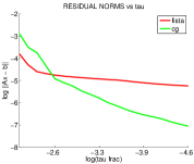
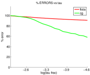
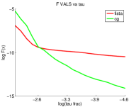
Figure 4: Averaged quantities along the regularization curve for matrix types I,II,III. Residual norms $||Ax_{\tau}-b||_{2}$, percent errors $100\frac{||x_{\tau}-x||_{2}}{||x||_{2}}$, and $\ell_{1}$ functional values $F_{1}(x_{\tau})$ versus decreasing $\tau$ (fraction of $||A^{T}b||_{\infty}$) for FISTA and CG.

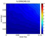
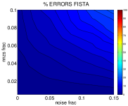
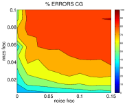
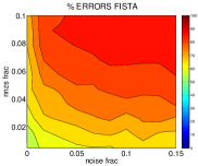
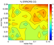
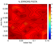
Figure 5: Contour plots for minimum percent errors over all $\tau$’s along the regularization curve at different combinations of nonzeros and noise fractions for matrix types I,II,III.

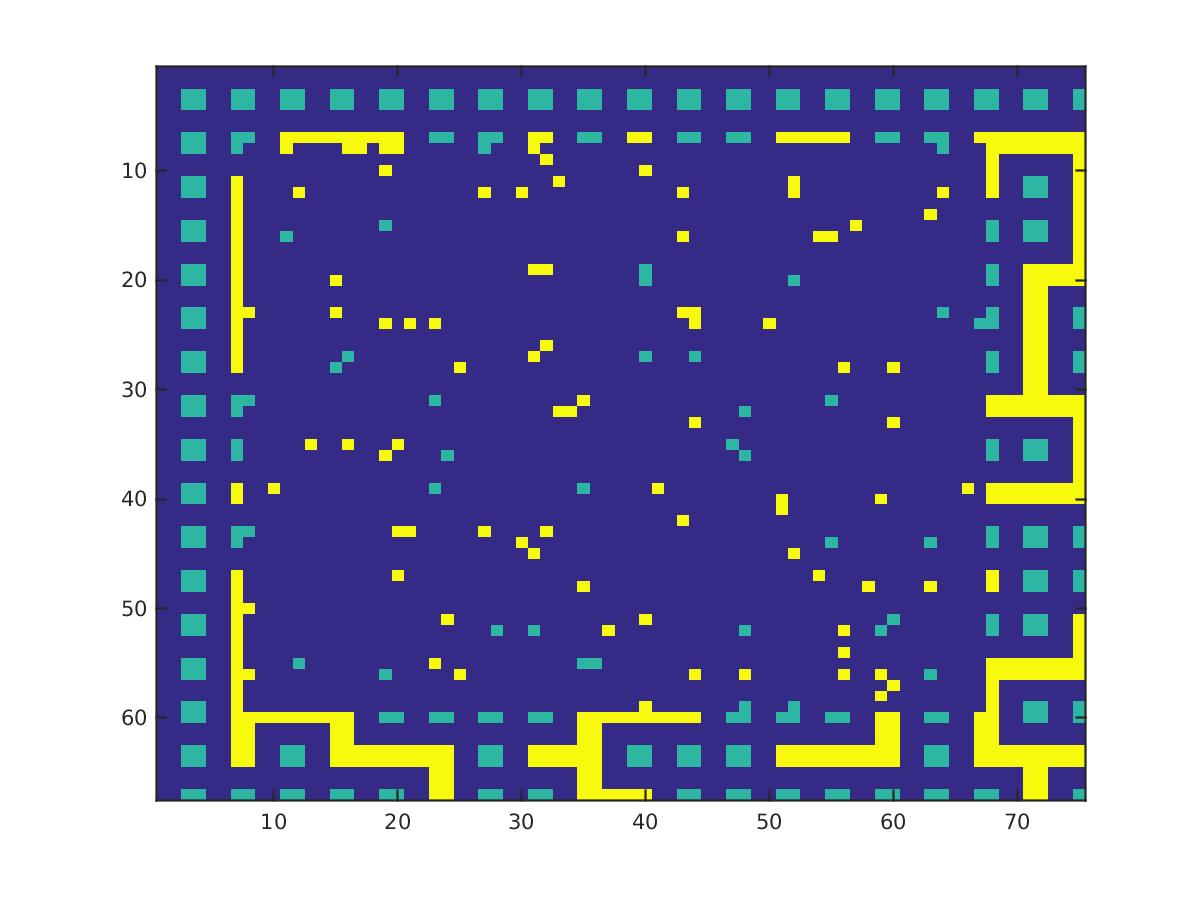
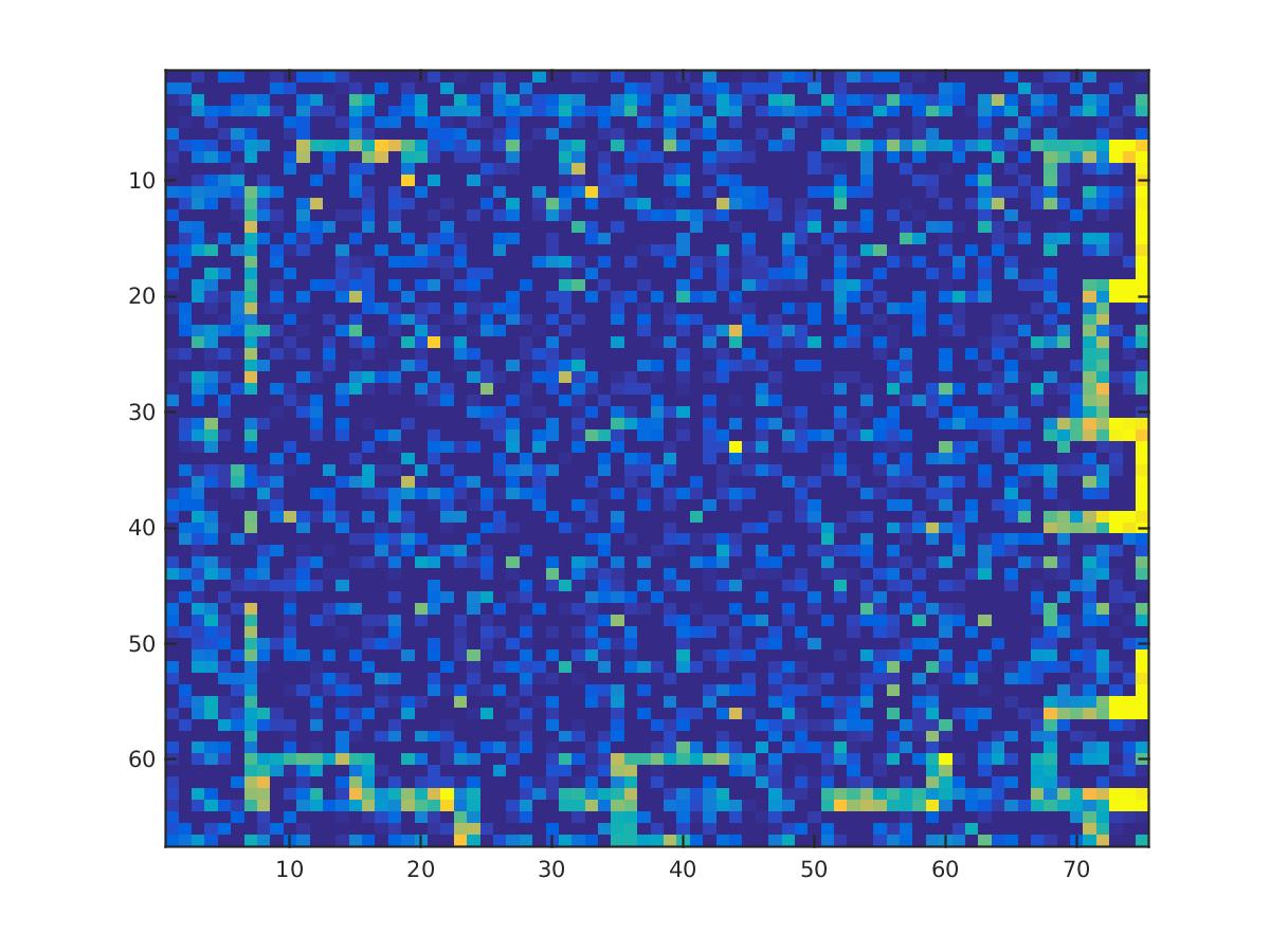
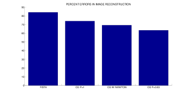
Figure 6: Image reconstruction for a $5025$ pixel image sampled via a random sensing matrix of size $5000\times 5025$ with rapidly decaying singular values, applied to the noisy version of the image. Row 1: original and noisy image. Row 2: recovered images using FISTA, CG (with $p=1$), CG with Newton’s method (with $p=1$), and CG (with $p=0.83$) run for $100$ iterations at each $\tau$ (FISTA) and at $50$ iterations (CG). Row 3: bar plot of percent errors (recovery error between recovered and original image) for the different algorithms.

5 Conclusions

In this article, we proposed new convolution based smooth approximations for the absolute value function $g(t)=|t|$ using the concept of approximate mollifiers. We established convergence results for our approximation in the $L^{1}$ norm. We applied the approximation to the minimization of the non-smooth functional $F_{p}(x)$ which arises in sparsity promoting regularization (of which the popular $\ell_{1}$ functional is a special case for $p=1$) to construct a smooth approximation $H_{p,\sigma}(x)$ of $F_{p}(x)$ and derived the gradient and Hessian of $H_{p,\sigma}(x)$.

We discussed the use of the nonlinear CG algorithm and higher order algorithms (like Newton’s method) which operate with the smooth $H_{p,\sigma}(x)$, $\nabla H_{p,\sigma}(x)$, $\nabla^{2}H_{p,\sigma}(x)$ functions instead of the original non-smooth functional $F_{p}(x)$.

We observe from the numerics in Section 4 that in many cases, in a small number of iterations, we are able to obtain better results than FISTA can for the $\ell_{1}$ case (for example, in the presence of high noise). We also observe that when $p<1$ but not too far away from one (say $p\approx 0.9$) we can sometimes obtain even better reconstructions in compressed sensing experiments.

The simple algorithms we show maybe useful for larger problems, where one can afford only a small number of iterations, or when one wants to quickly obtain an approximate solution (for example, to warm start a thresholding based method). The presented ideas and algorithms can be applied to design more complex algorithms, possibly with better performance for ill-conditioned problems, by exploiting the wealth of available literature on conjugate gradient and other gradient based methods. Finally, the convolution smoothing technique which we use is more flexible than the traditional mollifier approach and maybe useful in a variety of applications where the minimization of non-smooth functions is needed.

References

- [1] Milton Abramowitz and Irene A. Stegun, editors. Handbook of mathematical functions with formulas, graphs, and mathematical tables. A Wiley-Interscience Publication. John Wiley & Sons, Inc., New York; National Bureau of Standards, Washington, DC, 1984.
- [2] Amir Beck and Marc Teboulle. A fast iterative shrinkage-thresholding algorithm for linear inverse problems. SIAM J. Imaging Sci., 2(1):183–202, 2009.
- [3] Amir Beck and Marc Teboulle. Smoothing and first order methods: a unified framework. SIAM J. Optim., 22(2):557–580, 2012.
- [4] Rick Chartrand. Fast algorithms for nonconvex compressive sensing: Mri reconstruction from very few data. In Int. Symp. Biomedical Imaing, 2009.
- [5] Rick Chartrand and Valentina Staneva. Restricted isometry properties and nonconvex compressive sensing. Inverse Problems, 24(3):035020, 14, 2008.
- [6] John T. Chu. On bounds for the normal integral. Biometrika, 42(1/2):pp. 263–265, 1955.
- [7] I. Daubechies, M. Defrise, and C. De Mol. An iterative thresholding algorithm for linear inverse problems with a sparsity constraint. Communications on Pure and Applied Mathematics, 57(11):1413–1457, 2004.
- [8] Zdzisław Denkowski, Stanisław Migórski, and Nikolas S. Papageorgiou. An introduction to nonlinear analysis: theory. Kluwer Academic Publishers, Boston, MA, 2003.
- [9] David L. Donoho. For most large underdetermined systems of linear equations the minimal -norm solution is also the sparsest solution. Comm. Pure Appl. Math., 59(6):797–829, 2006.
- [10] Heinz W. Engl, Martin Hanke, and A. Neubauer. Regularization of Inverse Problems. Springer, 2000.
- [11] Norman L. Johnson, Samuel Kotz, and N. Balakrishnan. Continuous univariate distributions. Vol. 2. Wiley Series in Probability and Mathematical Statistics: Applied Probability and Statistics. John Wiley & Sons, Inc., New York, second edition, 1995. A Wiley-Interscience Publication.
- [12] L. Landweber. An iteration formula for Fredholm integral equations of the first kind. Amer. J. Math., 73:615–624, 1951.
- [13] I. Loris, M. Bertero, C. De Mol, R. Zanella, and L. Zanni. Accelerating gradient projection methods for -constrained signal recovery by steplength selection rules. Applied and Computational Harmonic Analysis, 27(2):247 – 254, 2009.
- [14] Hosein Mohimani, Massoud Babaie-Zadeh, and Christian Jutten. A fast approach for overcomplete sparse decomposition based on smoothed norm. IEEE Trans. Signal Process., 57(1):289–301, 2009.
- [15] Jorge Nocedal and Stephen J. Wright. Numerical optimization. Springer Series in Operations Research and Financial Engineering. Springer, New York, second edition, 2006.
- [16] E. Polak and G. Ribière. Note sur la convergence de méthodes de directions conjuguées. Rev. Française Informat. Recherche Opérationnelle, 3(16):35–43, 1969.
- [17] B.T. Polyak. The conjugate gradient method in extremal problems. {USSR} Computational Mathematics and Mathematical Physics, 9(4):94 – 112, 1969.
- [18] J. R. Shewchuk. An Introduction to the Conjugate Gradient Method Without the Agonizing Pain. Technical report, Pittsburgh, PA, USA, 1994.
- [19] N. Z. Shor, Krzysztof C. Kiwiel, and Andrzej Ruszcayǹski. Minimization Methods for Non-differentiable Functions. Springer-Verlag New York, Inc., New York, NY, USA, 1985.
- [20] Vikas Sindhwani and Amol Ghoting. Large-scale distributed non-negative sparse coding and sparse dictionary learning. In Proceedings of the 18th ACM SIGKDD International Conference on Knowledge Discovery and Data Mining, KDD ’12, pages 489–497, New York, NY, USA, 2012. ACM.
- [21] Albert Tarantola and Bernard Valette. Inverse Problems = Quest for Information. Journal of Geophysics, 50:159–170, 1982.