Probing the interstellar medium of NGC 1569 with Herschel

Abstract

NGC 1569 has some of the most vigorous star formation among nearby galaxies. It hosts two super star clusters (SSCs) and has a higher star formation rate (SFR) per unit area than other starburst dwarf galaxies. Extended emission beyond the galaxy’s optical body is observed in warm and hot ionised and atomic hydrogen gas; a cavity surrounds the SSCs. We aim to understand the impact of the massive star formation on the surrounding interstellar medium in NGC 1569 through a study of its stellar and dust properties. We use Herschel and ancillary multiwavelength observations, from the ultraviolet to the submillimeter regime, to construct its spectral energy distribution, which we model with magphys on $\sim$300 pc scales at the SPIRE 250 $\mu$m resolution. The multiwavelength morphology shows low levels of dust emission in the cavity, and a concentration of several dust knots in its periphery. The extended emission seen in the ionised and neutral hydrogen observations is also present in the far–infrared emission. The dust mass is higher in the periphery of the cavity, driven by ongoing star formation and dust emission knots. The SFR is highest in the central region, while the specific SFR is more sensitive to the ongoing star formation. The region encompassing the cavity and SSCs contains only 12 per cent of the dust mass of the central starburst, in accord with other tracers of the interstellar medium. The gas–to–dust mass ratio is lower in the cavity and fluctuates to higher values in its periphery.

1 Introduction

The most extreme form of massive star formation occurring in galaxies is in the form of super star clusters (SSCs). These are very luminous, with L_V between 10⁶–10⁸ L_⊙, massive, with stellar masses higher than 10⁵M_⊙, and very compact, with effective radii less than 5 pc (Billett et al., 2002; O’Connell, 2004, and references therein). The star formation conditions during gravitational interactions favour the formation of SSCs (Larsen, 2010; Billett et al., 2002). SSCs are important as they have been considered as the younger analogues to the old Galactic globular clusters (GCs) and show that the formation of very massive stellar clusters is continuous as a function of time (Larsen, 2010; de Grijs et al., 2005; O’Connell, 2004).

The most prominent example of a nearby dwarf galaxy that contains one SSC is the Large Magellanic Cloud (LMC; with R 136 in the 30 Doradus H ii region; Massey & Hunter 1998). The next nearest extragalactic resolved SSCs in a dwarf galaxy are hosted in NGC 1569 (e.g., O’Connell et al., 1994; Grocholski et al., 2012) and NGC 4214 (e.g., Leitherer et al., 1996; Drozdovsky et al., 2002; Dopita et al., 2010), at similar distances ($\sim$3 Mpc). Our focus in the current work is placed on NGC 1569, a starburst low–metallicity dwarf irregular galaxy, with an oxygen abundance of 8.02$\pm$0.02 (in the Pilyugin & Thuan 2005 scale adapted from Kobulnicky & Skillman 1997; Madden et al., 2013), and a stellar metallicity of Z = 0.1–0.2 Z_⊙ (Grocholski et al., 2008; Aloisi et al., 2001). At a distance of 2.96$\pm$0.22 Mpc (Grocholski et al., 2012), it is a member of the IC 342 group of galaxies, and the intense starburst may have been triggered by the gravitational interactions with other galaxy group members or with a nearby low-mass H i companion (Johnson, 2013; Hunter et al., 2012; Holwerda et al., 2013; Jackson et al., 2011; Stil & Israel, 1998).

NGC 1569 hosts two SSCs, one of which consists of two components (de Marchi et al., 1997; O’Connell et al., 1994; Hunter et al., 2000). The star formation in the central starburst is concentrated in three distinct events within the last 1–2 Gyr, with the most recent between 8–27 Myr ago (Angeretti et al., 2005). In the outer parts of the galaxy, the star formation peaked around 500 Myr ago along with subsequent recent bursts of lower intensity and duration (Grocholski et al., 2012). SSC A and SSC B formed during the last bursts of star formation, having ages of the order of 7 Myr and 10-20 Myr (Hunter et al., 2000; Larsen et al., 2008). NGC 1569 contains, apart from the two SSCs, a large number of young ($\sim$30 Myr), compact and massive star clusters (Hunter et al., 2000; Anders et al., 2004), similar to the ones found in the LMC (e.g., Hunter et al., 2003). Even though NGC 1569 and LMC are galaxies that are gravitationally interacting (Besla et al., 2012; Putman et al., 1998; Johnson, 2013; Stil & Israel, 1998), the formation of compact star clusters in galaxies is not unique to interacting / merging galaxies (Larsen, 2010).

In NGC 1569, the winds of the SSCs have profoundly impacted the interstellar medium (ISM) around them leading to a complex morphology (Westmoquette & et al., 2007b), including a cavity evident in H i and H $\alpha$ (Israel & van Driel, 1990; Hunter et al., 2000). Studies of the hot and warm ionised gas reveal filaments of ionised gas, expanding shells, superbubble kinematics and galactic scale outflows (Heckman et al., 1995; Martin et al., 2002; Westmoquette et al., 2008, and references therein). Moreover, Waller (1991) detects H ii regions in the periphery of the cavity, especially in the East and West of SSC A, while Taylor et al. (1999) detect giant molecular clouds in the West and North–West direction of the SSC A. With a diameter of $\sim$200 pc, the H i / H $\alpha$ cavity is a strong manifestation of the impact of the massive star formation on the ISM. This cavity is reminiscent of the giant H ii region NGC 604 in M 33, which also presents a complex ISM morphology powered by a cluster of massive stars in its centre (Martínez-Galarza et al., 2012, and references therein).

Several feedback mechanisms have been proposed to explain the discrepancy between observed and theoretically predicted numbers of low-mass galaxies (Benson et al., 2003; Sawala et al., 2010, and references therein). Attributed to feedback processes is also the mixing of metals with the metal–poor ISM, while galactic-scale outflows further drive metals to the intergalactic medium to enrich it (Recchi, 2014; Kawata et al., 2014, and references therein). The intriguing observation of NGC1569’s SSCs clearing out the ISM and forming the cavity seen in H i and H $\alpha$ leaves us with the following questions: how are the dust properties distributed across the central starburst, and especially in the cavity region? how do the dust properties relate to the ongoing and embedded star formation? how does the dust emission relate to the other ISM tracers of the warm ionised and atomic hydrogen gas? Dust is an important component of a galaxy’s ISM, and a significant amount of a galaxy’s bolometric luminosity is emitted in the infrared, through reprocessing by dust of the radiation emitted by massive stars. The sensitivity and spatial resolution offered with Herschel, together with the new wavelength coverage in the submillimeter (submm), allow a new study to investigate these questions, in much greater detail than before. Our study primarily focuses on understanding the stellar and dust properties in the cavity and the interplay between them, as well as across the central starburst.

Galliano et al. (2003) and Lisenfeld et al. (2002) focus on the global ISM properties of NGC 1569, consistently modelling the mid-infrared (MIR) to millimetre observations of ISO, IRAS, SCUBA/JCMT and MAMBO/IRAM multiwavelength dust spectral energy distribution (SED), finding an emission in excess compared to the model predictions at submm wavelengths, often referred to as submm excess. Rémy-Ruyer et al. (2013) and Rémy–Ruyer et al. (in prep.) use Herschel observations along with both modified black–body fits to the SED and detailed SED modelling to study the global dust properties, as well as the gas–to–dust mass ratio (Rémy-Ruyer et al., 2014), for a sample of low–metallicity dwarf galaxies (Madden et al., 2013), including NGC 1569.

Table 1: Properties of NGC 1569.

Quantity	Value (ref.)
Type	IBm
RA (J2000.0)	$04^{h}30^{m}49.0^{s}$
Dec (J2000.0)	$+64^{\circ}50^{\prime}53.0^{\prime\prime}$
$\rm E(B-V)$ (mag)	0.51 (1)
$(m-M)_{0}$ (mag)	27.52$\pm$0.14 (2)
Distance (Mpc)	2.96$\pm$0.22 (2)
D25($\arcsec$)	216 (3)
MV (mag)	$-18.2$ (4)
M⋆ (M☉)	2.8$\times$108 (5)
M${}_{\mbox{H\,{\sc i}}}$ (M☉)	2.5$\times$108 (4)
MHα (M☉)	1.3$\times$105 (6)
M${}_{H_{2}}$ (M☉)	2$\times$106 (7)
MD (M☉)	2.8${}^{+1.5}_{-1.4}\times$105 (8)
12+log(O / H)	8.02$\pm$0.02 (9)

In the present study, we consider the star and dust properties on a pixel–by–pixel basis and in two regions via modelling the observed 0.15 $\mu$m to 500 $\mu$m SED using magphys (da Cunha et al., 2008), and we compare our findings with other ISM tracers, such as the warm ionised and atomic hydrogen gas and the CO–traced molecular gas. A detailed examination of the ISM properties in the central region of the starburst of NGC 1569 will provide us with valuable insights to lend interpretation to the properties of more distant starburst galaxies. We assume a distance modulus of 27.52$\pm$0.14 mag or a distance of 2.96$\pm$0.22 Mpc (based on the tip of the red giant branch and reddening consistent with the Burstein & Heiles (1982) value; Grocholski et al., 2012). Table 1 lists the basic properties of NGC 1569. With the SED modelling on a pixel–by–pixel basis, the smallest spatial scale we are probing is 21$\arcsec$ or 294 pc. The results of the SED modelling on the dust and star properties are model–dependent and thus tied to the scale defined by magphys. The flux densities of the observations considered here are in the Vega photometric system, except from the GALEX data which are in the AB photometric system.

2 Observations & analysis

Table 2: Wavelength coverage and adopted calibration errors.

Telescope / Filter	$\lambda$ ($\mu$m)	FWHM	Ref.	Error	Ref.
GALEX / FUV	0.15	4.2$\arcsec$	1	5%	1
GALEX / NUV	0.23	5.3$\arcsec$	1	3%	1
KPNO / B	0.44	18.2$\arcsec$	2	3%	2
KPNO / V	0.54	18.2$\arcsec$	2	3%	2
2MASS / J	1.25	2.5$\arcsec$	3	3%	3
2MASS / H	1.65	2.5$\arcsec$	3	3%	3
2MASS / KS	2.17	2.5$\arcsec$	3	3%	3
WISE / W1	3.4	8.4$\arcsec$	4	2.4%	4
WISE / W2	4.6	9.2$\arcsec$	4	2.8%	4
WISE / W3	12	11.4$\arcsec$	4	4.5%	4
WISE / W4	22	18.6$\arcsec$	4	5.7%	4
Spitzer / IRAC	3.6	1.7$\arcsec$	5	8.3%	5
Spitzer / IRAC	4.5	1.7$\arcsec$	5	7.1%	5
Spitzer / IRAC	5.8	1.9$\arcsec$	5	22.1%	5
Spitzer / IRAC	8.0	2.0$\arcsec$	5	16.7%	5
Spitzer / MIPS	24	6.0$\arcsec$	6	4%	6
Herschel / PACS	70	5.8$\arcsec$	7	5%	7
Herschel / PACS	100	7.1$\arcsec$	7	5%	7
Herschel / PACS	160	11.2$\arcsec$	7	5%	7
Herschel / SPIRE	250	18.2$\arcsec$	7	7%	7
Herschel / SPIRE	350	25.0$\arcsec$	7	7%	7
Herschel / SPIRE	500	36.4$\arcsec$	7	7%	7

While this study is motivated by Herschel observations, we use numerous archival data sets to cover the ultraviolet (UV) to the infrared (IR) and submm wavelength regime. We use Herschel PACS (Poglitsch et al., 2010) and SPIRE (Griffin et al., 2010) imaging observations to probe the far–IR (FIR) and submm part of the spectrum, from 70 $\mu$m to 500 $\mu$m; these data are part of the Dwarf Galaxy Survey (PI S. Madden; Madden et al. 2013), and we refer to Rémy-Ruyer et al. (2013) for more information on the data reduction techniques. The ancillary observations that we use for our study are taken from publicly available archives. Table 2 lists the available multiwavelength data set coverage.

The far-UV (FUV; 1350–1750 Å) and near-UV (NUV; 1750–2750 Å) images come from GALEX (Martin et al., 2005), as part of the GALEX Nearby Galaxies Survey (Gil de Paz et al., 2007), and are retrieved through the archive as background subtracted intensity maps. The optical part of the data consist of broadband B and V data adopted from Hunter & Elmegreen (2006). The near–IR part of the spectrum is covered with data from the 2MASS (Skrutskie et al., 2006) archive in the J, H, Ks filters. For the MIR and FIR wavelength regime, we use WISE data (in the W1, W2, W3, W4 filters; Wright et al., 2010), as well as Spitzer data (Werner et al., 2004), both IRAC (in the 3.6, 4.5, 5.8 and 8.0 $\mu$m bands; Fazio et al., 2004) and MIPS (only 24 $\mu$m; Rieke et al., 2004). The WISE and IRAC data sets are retrieved through the NASA / IPAC Infrared Science Archive (IRSA), while the MIPS data are from Bendo et al. (2012).

All images are treated initially in their native pixel scales, where the unit conversion of the flux density takes place from the native unit to Jy / pixel. Subsequently, we use SExtractor (Bertin & Arnouts, 1996) in each image to estimate the background flux density and subtract it. We use the segmentation image created by SExtractor, in order to mask the images from the detected sources. The segmentation image is the input image with all detected point and extended sources assigned to positive pixel values and the remaining background structure set to zero pixel values. We then estimate the background flux density from the masked image. The segmentation image is also used to mask the foreground stellar contamination. The GALEX, 2MASS and MIPS images are already background–subtracted.

We then correct the UV–to–MIR images for Galactic foreground extinction:

$$F_{\rm i}=F_{\rm obs}10^{0.4E(B-V)[{\rm\kappa}({\rm\lambda}-V)+R_{V}]},$$ (1)

where F_i is the flux density corrected for foreground extinction, F_obs is the observed flux density, E(B$-$V) is the colour excess, R_V = 3.1, and ${\rm\kappa}({\rm\lambda}$-V) is the extinction curve. In order to estimate the ${\rm\kappa}({\rm\lambda}$-V) values at the optical bands, B and V, we use the Galactic extinction curve of Fitzpatrick (1999), while for the near–IR to MIR bands (2MASS bands; WISE W1, W2, & W3 bands; IRAC 3.6, 4.5, 5.8, & 8.0 $\mu$m bands) we use the one from Indebetouw et al. (2005). The GALEX data are corrected for the Galactic foreground extinction using the selective extinction A_FUV / E(B$-$V) = 8.29 and A_NUV / E(B$-$V) = 8.18 (Seibert et al., 2005). We adopt for NGC 1569 a Galactic foreground reddening E(B$-$V) = 0.51 mag (Burstein & Heiles, 1982), which gives a Galactic foreground extinction A_V = 1.58 mag. The motivation for this choice of reddening is from past studies on the internal extinction across the galaxy, which found the total reddening, i.e. Galactic foreground plus internal, to vary between 0.56 to 0.80 mag (Pasquali et al., 2011; Relaño et al., 2006; Devost et al., 1997; Kobulnicky & Skillman, 1997; Calzetti et al., 1996). We do not perform internal extinction corrections to the data set for the SED modelling procedure, while in the occasion where these are performed then this is explicitly noted each time.

Table 3: Applied colour corrections.

Camera	Power law index	Colour correction
W1 3.4 $\mu$m	1	0.9961
W2 4.6 $\mu$m	1	0.9976
W3 12 $\mu$m	$-$2	1
W4 22 $\mu$m	$-$2	1
IRAC 3.6 $\mu$m	1	1.0037
IRAC 4.5 $\mu$m	1	1.0040
IRAC 5.8 $\mu$m	$-$2	1.0052
IRAC 8 $\mu$m	$-$2	1.0111
MIPS 24 $\mu$m	$-$2	0.960
PACS 70 $\mu$m	$-$2	1.016
PACS 100 $\mu$m	2	1.034
PACS 160 $\mu$m	2	1.075
SPIRE 250 $\mu$m	2	0.9878
SPIRE 350 $\mu$m	2	0.9890
SPIRE 250 $\mu$m	2	1.0128

We additionally perform colour corrections to the WISE, Spitzer, and Herschel images. Colour corrections are necessary in the case of wide filters where the spectral shapes of the sources used in the calibration process are different than the spectral shape of the targets under study. We assume power law indexes and colour corrections, as listed in Table 3. The power law indexes were determined using the galaxy’s SED (in an aperture similar as the one used in Sec. 7 for the central starburst region), and solving the equation F${}_{\nu}\,\propto\,\nu^{\alpha}$ for $\alpha$, where F_ν is the specific flux density, $\nu$ is the frequency, and $\alpha$ is the power law index. The power law index was determined: for W1, W2, IRAC 3.6 $\mu$m, and IRAC 4.5 $\mu$m solving for $\alpha$ the above equation at the wavelengths in the 2MASS K_S band and in the W2 band; for IRAC 5.8 $\mu$m, IRAC 8 $\mu$m, W3, W4, MIPS 24 $\mu$m, and PACS 70 $\mu$m solving for $\alpha$ at the wavelengths in the W2 and PACS 70 $\mu$m; for the remaining bands, solving for $\alpha$ at the wavelengths in the PACS 100 $\mu$m and SPIRE 500 $\mu$m. The colour corrections listed in Table 3 are taken from Wright et al. (2010) for WISE, from the IRAC Instrument Handbook (version 2.0.3; 2013) for IRAC, from the MIPS Instrument Handbook (version 3.0; 2011) for MIPS, from Poglitsch et al. (2010) for PACS, and from the SPIRE Data Reduction Guide (version 2.3; 2013) for SPIRE. The colour correction of the SPIRE data additionally includes beam effect corrections which also depend on the spectral shape of the source of the emission. Finally, we apply extended source corrections to the IRAC bands, as recommended in the IRAC Instrument Handbook (version 2.0.3; 2013), using the surface brightness corrections listed in Table 4.9.

After these corrections are applied, we register the – background, galactic foreground extinction, and colour–corrected – images to a common world coordinate system, centred on the galaxy and covering the region of 294$\arcsec$ $\times$ 294$\arcsec$ ($\sim$ 4116 pc $\times$ 4116 pc, at our adopted distance). The final step of the image processing is the convolution of all images to a common point-spread function (PSF), using the convolution kernels of Aniano et al. (2011). For bands without a convolution kernel in the Aniano et al. (2011) database (the 2MASS and B, V data sets), we use a Gaussian kernel with FWHM taken from Aniano et al. (2011, Column 7 of their Table 6).

In order to retain the best spatial resolution possible for the purposes of our study, as well as to fully exploit the whole Herschel imaging data set, we convolve the available imaging to two different PSFs. First, to the PSF of the SPIRE 250 $\mu$m band, a FWHM of 18.2$\arcsec$, thus keeping all imaging up to this band for our analysis. Second, to the PSF of the SPIRE 500 $\mu$m band, which corresponds to 36.4$\arcsec$.

Each set of the convolved images is, then, re-sampled to a 21$\arcsec$ pixel size for the set of images convolved to the SPIRE 250 $\mu$m PSF, and 42$\arcsec$ for the set of images convolved to the SPIRE 500 $\mu$m PSF. The re–sampled pixel sizes are larger than the common PSF, in order to derive statistically independent properties. In the former case, the pixel size probes the ISM properties in spatial scales equivalent to 294 pc, which is larger than the size of the H i / H $\alpha$ cavity (a diameter of 198 pc at our adopted distance; Hunter et al. 2000). The data set convolved to the SPIRE 500 $\mu$m PSF consists of a total of 22 images, exploiting the full Herschel imaging, while the data set of images convolved to the SPIRE 250 $\mu$m PSF consists of a total of 20 images, i.e., dropping the two longer wavelength SPIRE bands. Several steps of the image processing have been performed using Imagecube (Taylor, Lianou, & Barmby 2013; Lianou & et al., 2013a).

The photometric uncertainties are derived directly on the convolved and re–sampled images, on a pixel–by–pixel basis, using the approach of Aniano et al. (2012). These authors model the SEDs of two spiral galaxies (NGC 628 & NGC 6946) drawn from the KINGFISH sample (Kennicutt et al., 2011) using the dust model of Draine & Li (2007) and deriving the dust properties both on global and local scales. Here, we assume background variations and calibration errors as the main source of uncertainties. The background variations have been estimated on the final images, after masking the galaxy with the SExtractor segmentation image. In this way, background pixels are defined, and eq. D2 of Aniano et al. (2012) has been used to estimate the background noise on a pixel–by–pixel basis. The calibration errors adopted are listed in Table 2. The two uncertainties of the background variation and calibration errors are then added in quadrature.

3 Multiwavelength emission morphology

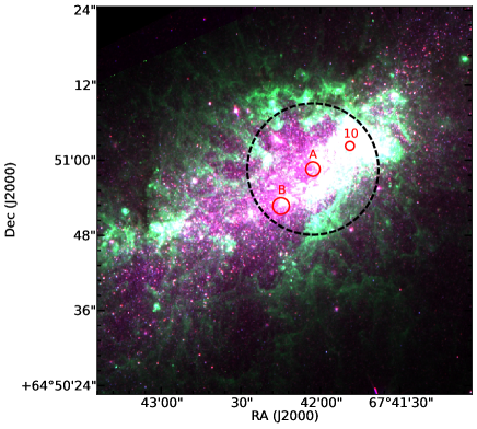
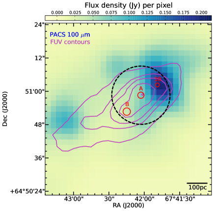
Figure 1: Upper panel: Three-colour image of NGC 1569 showing the inner 60$\arcsec$ $\times$ 60$\arcsec$ region, and composed of HST / ACS images in the following filters: F606W (blue), H $\alpha$ (green), and F814W (red). The two SSCs and SC 10 are shown with the red solid circles, while the cavity region is shown with the black dashed circle (diameter of 21$\arcsec$ to match the one used in Sec. 7). The pixel scale of the three-colour image is 0.05$\arcsec$. Lower panel: PACS 100 $\mu$m image of NGC 1569 shown in its native angular resolution (7.1$\arcsec$ FWHM) and covering the same region as in the upper panel. The contours are shown at the GALEX FUV native angular resolution (4.2$\arcsec$ FWHM), at the levels of 2.5 mJy, 1 mJy, 0.5 mJy, 0.3 mJy, and 0.1 mJy, going from the inner to the outer contour, respectively. The pixel scale is 2$\arcsec$. At the adopted distance of NGC 1569, 1$\arcsec$ corresponds to 14 pc.

The upper panel of Fig. 1 shows a three-colour image of NGC 1569 based on HST images (GO 10885; PI A. Aloisi; Grocholski et al. 2012) and focusing on the central starbursting area of 840 pc $\times$ 840 pc (60$\arcsec$ $\times$ 60$\arcsec$). SSC A, SSC B, and SC 10 are shown with their true angular sizes, 1.14$\arcsec$, 1.34$\arcsec$, and 0.71$\arcsec$, respectively (Hunter et al., 2000). The H $\alpha$ emission, which traces the ongoing star formation in timescales of about 10 Myr (Lee et al., 2011; Kennicutt & Evans, 2012), reveals the cavity (Hunter et al., 2000; Pasquali et al., 2011) that has been initially observed in H i (Israel & van Driel, 1990).

The cavity is centred on SSC A and has a diameter of 198 pc (Hunter et al., 2000), thus it extends to also contain SSC B. SSC A and SSC B have ages of 7 Myr and 10-25 Myr (Hunter et al., 2000; Larsen et al., 2008), respectively, while their masses range between 6–7$\times$10⁵ M_⊙ (Grocholski et al., 2012; Larsen et al., 2008). SC 10 is located at the edges of the cavity and towards its North–West direction, where giant molecular clouds have been observed together with ongoing star formation in an embedded phase (Tokura et al., 2006; Taylor et al., 1999; Waller, 1991). SC 10, which is not considered an SSC, has a stellar mass of $\sim$10³ M_⊙ and consists of two components, both with young ages: one of 5–7 Myr, and another with less than 5 Myr (Westmoquette & et al., 2007a).

The lower panel of Fig. 1 shows contours of the GALEX FUV emission overlaid on the PACS 100 $\mu$m map. The PACS 100 $\mu$m emission traces the warm dust, while the FUV emission reveals the recent star formation occurring at a timescale of less than 100 – 300 Myr (e.g., Lee et al., 2011; Calzetti, 2013). The emission from these young stars dominates the region inside the H i / H $\alpha$ cavity, where the dust emission at 100 $\mu$m seems less prominent. There are several dust knots revealed at 100 $\mu$m, which are located outside the very central starbursting region and mark the periphery of the cavity. At the location of these knots, several H ii regions and giant molecular clouds are found (Waller, 1991; Taylor et al., 1999; Pasquali et al., 2011; Johnson et al., 2012). These molecular clouds host embedded star formation (Tokura et al., 2006; Westmoquette & et al., 2007a; Clark et al., 2013). The brightest of these dust knots spatially coincides with SC 10 and extends to its north, northwest, and southwest. At the location of the brightest dust knot, the onset of an H $\alpha$ feature has been observed by Waller (1991), while Taylor et al. (1999) report that the detected molecular clouds are located in the interface region between the cold atomic gas phase and the hot gas, as due to the shocks of the outflow. Hong et al. (2013) and Westmoquette & et al. (2007b) identify at the same location shocks due to stellar feedback and the outflow. These reports from the literature may suggest that the bright dust knot in the northwest to the SSC A is due to the embedded and ongoing star formation and the complex ISM dynamics due to the outflow.

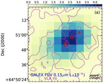
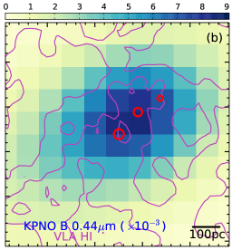
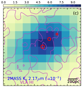
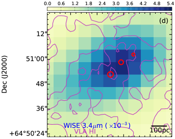
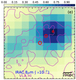
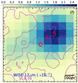
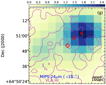
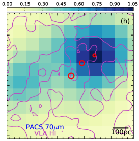
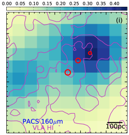
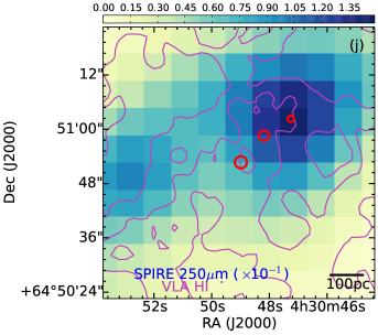
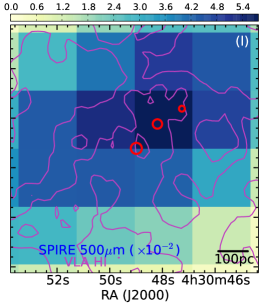
Figure 2: Multi-wavelength flux density maps. The unit of the colorbar is Jy / pixel. The maps up to SPIRE 250 $\mu$m are in the resolution of the SPIRE 250 $\mu$m PSF (18.2$\arcsec$ FWHM), while the remaining two maps are in the resolution of the SPIRE 500 $\mu$m PSF (36.4$\arcsec$ FWHM). Contours show the H i emission, with levels ranging from 2 mJy/pixel$\times$km/sec to 9 mJy/pixel$\times$km/sec with a step of 3.5 mJy/pixel$\times$km/sec. The field of view is 60$\arcsec$ $\times$ 60$\arcsec$. Red solid circles indicate the location of the SSCs and SC 10.

Fig. 2 shows the flux density maps of the images at representative filters we use in our SED analysis, so as to illustrate the spatial distribution of their emission. The GALEX FUV emission (panel a) reveals a rather homogeneous and centrally concentrated spatial distribution, which is dominated by the emission of the young stars. The optical B–band (panel b), 2MASS K_s (panel c) and WISE 3.4 $\mu$m (panel d) emission, which trace the young as well as the more evolved stars, show a similar distribution as the FUV emission, albeit more extended. A more confined distribution of the FUV emission as compared to the optical and MIR is also reflected in the corresponding disk scale lengths reported in Zhang et al. (2012). The emission in the IRAC 8 $\mu$m (panel e) and WISE 12 $\mu$m (panel f) bands is sensitive to the hot dust from polycyclic aromatic hydrocarbons (PAHs), as well as the warm dust continuum. The emission in the MIPS 24 $\mu$m and up to the PACS 160 $\mu$m traces the warm dust (panels g to i), while the emission longwards to the SPIRE 250 $\mu$m (panels j to l) traces the cold dust. At the IRAC 8 $\mu$m and up to the SPIRE 250 $\mu$m, two dust knots are revealed, offset from the central region, as also seen in the warmer dust emitting at 100 $\mu$m discussed in Fig. 1.

The North–Western dust knot is bright at all bands longwards to the IRAC 8 $\mu$m, while the fainter dust emission knot to the southeast of SSC A becomes redder in the MIPS 24 $\mu$m (see also Fig. 4 in Wu et al., 2006) and in the PACS 70 $\mu$m map. The giant molecular clouds detected by Taylor et al. (1999) lie in the brightest North–Western dust knot seen in the warm and cold dust emission. At all MIR to FIR and submm wavelengths, where the angular resolution permits, dust knots coincide with the locations of the ongoing star formation in the periphery of the cavity, the latter indicated with the H i contours in Fig. 2. The SPIRE 350 and 500 $\mu$m maps show the coldest dust emission to be distributed over the whole body of NGC 1569. Any substructure in the coldest dust components is not well-resolved in these bands, thus making it challenging to reveal the source of heating.

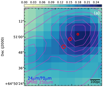
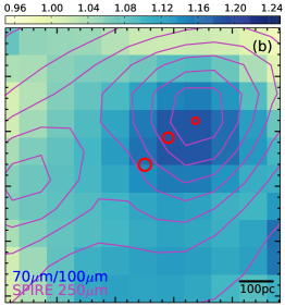
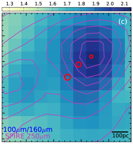
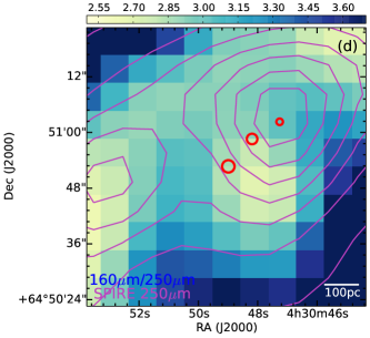
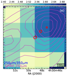
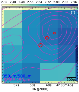
Figure 3: Flux density ratio maps for the FIR bands. Ratio maps shown up to SPIRE 250 $\mu$m are in its angular resolution (18.2$\arcsec$ FWHM), while the remaining maps are shown in the resolution of the SPIRE 500 $\mu$m PSF (36.4$\arcsec$ FWHM). Contours show the SPIRE 250 $\mu$m emission, with levels ranging from 130 to 10 mJy with a step of 20 mJy, per pixel. The field of view is 60$\arcsec$ $\times$ 60$\arcsec$. Red solid circles indicate the SSCs and SC 10.

Fig. 3 shows the flux density ratio maps of the FIR images. These ratio maps reveal overall warmer colours, i.e. having ratios larger than one, in all but the very first map (panel a). The ratio 24 $\mu$m / 70 $\mu$m (panel a) reveals a colder colour in the central starburst, with an increasing 24 $\mu$m emission in the North–Western dust knot.

Extended emission beyond the main optical body of NGC 1569 is seen at all Herschel wavelengths up to SPIRE 250 $\mu$m. The extended emission in the

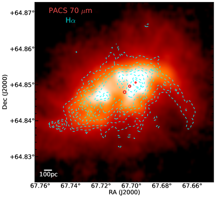
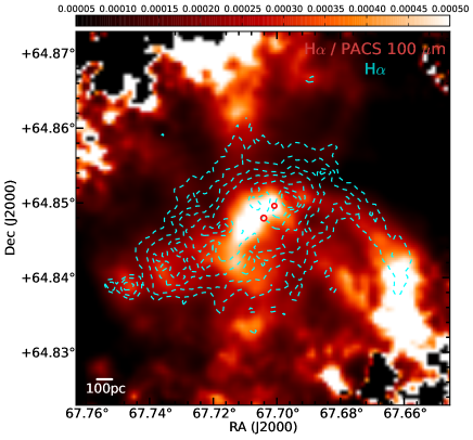
Figure 4: Left panel: PACS 70 $\mu$m map showing the extended emission within 180$\arcsec$ $\times$ 180$\arcsec$, with contours of H $\alpha$ overlaid in dashed cyan. White colour corresponds to higher emission. Right panel: H $\alpha$ / PACS 100 $\mu$m ratio map of the same region with the same contours overlaid as in the left panel. White colour corresponds to a higher flux density ratio. The location of the SSCs and SC 10 is indicated with the red solid circles.

PACS 70 $\mu$m map is shown in the left panel of Fig. 4. The emission is also evident in X-ray and H $\alpha$ observations and has been associated with larger scale galactic outflows (Heckman et al., 1995; Martin, 1998; Westmoquette et al., 2008). Such galactic outflows are seen in other nearby starburst galaxies (e.g., NGC 253, M 82; Westmoquette et al., 2011; Heckman et al., 1990), and recently shown for NGC 253 to be accompanied by molecular gas outflows (Bolatto et al., 2013), as well as associated with atomic hydrogen plumes (Boomsma et al., 2005). In the case of NGC 1569, its larger scale extended emission is also detected by the warm and cold dust components, from the PACS 70 $\mu$m to the SPIRE $250$ $\mu$m. The warm dust traced by the PACS 70 $\mu$m emission follows the H $\alpha$ morphology in the most extended structures seen, as shown with the contours overlaid of the H $\alpha$ emission (left panel of Fig. 4). The ratio of the warm ionised gas (traced with the H $\alpha$ emission) to the warm dust (traced with the 100 $\mu$m emission) reveals even more prominently the warm colour of the emission (higher ratio) at the sites of the extended emission, alternating by cooler colours (lower ratio) adjacent to the warm ionised gas marking the outflow.

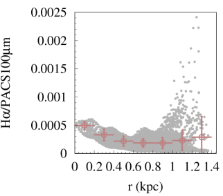
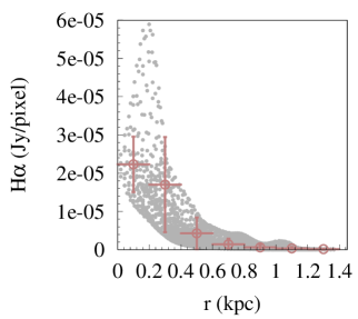
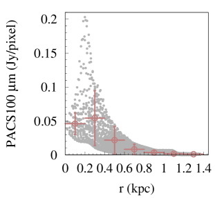
Figure 5: Left panel: H $\alpha$ / PACS 100 $\mu$m ratio profile. The red (darker) symbols are data binned within 0.2 kpc regions. Middle panel: PACS 100 $\mu$m flux density profile. The red (darker) symbols are data binned within 0.2 kpc regions. Right panel: H$\alpha$ flux density profile. The red (darker) symbols are data binned within 0.2 kpc regions. All data have been convolved to the PACS 100 $\mu$m PSF.

The same trends are revealed in the radial profiles shown in Fig. 5. The left panel shows the H $\alpha$ / PACS 100 $\mu$m ratio profile. There is the trend of a decreasing ratio with increasing galactocentric radius, with overall cooler colours. The colour, though, becomes warmer at the location of the extended emission, i.e. beyond $\sim$1 kpc. The middle and right panel of Fig. 5 show the flux density profiles of the H $\alpha$ and the 100 $\mu$m emission, respectively. The flux density enhancements in both profiles occur beyond $\sim$1 kpc and indicate the extended emission.

4 SED modelling with magphys

We derive the star formation and dust properties by using magphys (da Cunha et al., 2008) to model the observed multiwavelength SED of NGC 1569, initially on a pixel–by–pixel basis, and later on for two individual regions within the galaxy. Magphys is a simple, physically motivated model to interpret the SED of a galaxy and its basic characteristics are described in da Cunha et al. (2008). Magphys provides a consistent model for the emission of stars and dust to interpret the multiwavelength SEDs of galaxies and extract constraints on their stellar populations and ISM properties. The magphys model uses the Bruzual & Charlot (2003) stellar population synthesis to model the spectral evolution of a galaxy, together with the model of Charlot & Fall (2000) to describe the attenuation of stellar emission by dust in the diffuse ISM and in the stellar birth clouds (BCs), which are then coupled to the dust emission model of da Cunha et al. (2008) via conservation of the energy for the dust absorbed in the BCs and diffuse ISM and re-radiated in the IR. No detailed modelling of the physical properties of the dust grains is performed in magphys, with the main components of the IR emission briefly described below.

There are two basic steps involved in the panchromatic SED modelling with magphys. The first step is the construction of a library of model SEDs ranging in rest–frame wavelength from 912 Å to 1 mm, with which the observed SEDs are fitted via $\chi^{2}$–minimisation. The second step is to construct the marginalised likelihood distribution for each physical parameter of the observed galaxy, through the comparison of the observed and model SEDs. An assumption made in the modelling is that there is contribution of only starlight to the heating of the diffuse ISM, thus ignoring any AGN component. The total dust mass derived in magphys includes the dust mass contributed by warm dust in the stellar BCs and in the diffuse ISM, as well as the dust mass contributed by cold dust in the diffuse ISM. Components of cold dust clumps not heated by starlight are not included in the modelling with magphys. Such quiescent cold clumps of dust have been uncovered with radiative transfer modelling of disk galaxies and are proposed in order to reconcile the observed FIR and submm SED (e.g., de Looze et al., 2012; Holwerda et al., 2012; Bianchi & Xilouris, 2011; Baes et al., 2010).

The library of model SEDs covers a wide range of star formation histories (SFHs), metallicities and dust contents and is constructed using two components. The first component of the model library involves the set of stellar population spectra, drawn from the Bruzual & Charlot (2003) stellar population synthesis code and covering the wavelength range of 912 Å to 160 $\mu$m. The second component of the model library involves the dust emission spectra, for which dust emission from the stellar BCs and the diffuse ISM is taken into account. These two components of the model library are then linked together via energy conservation, in order to construct the 912 Å  to 1 mm model SED and fit this to the observed SED.

The first component of the model SED library involves the stellar population spectra which are described by:

• Parameters related to the SFH assuming the following to hold simultaneously: (1) a continuous SFR, described by the age of the galaxy, t_form, uniformly distributed between 0.1 to 13.5 Gyr; (2) a star formation timescale, $\gamma$, uniform in the interval 0 to 0.6 Gyr^-1 and exponentially dropping to zero around 1 Gyr^-1; (3) bursts of star formation superimposed on the continuous SFR, such that 50 per cent of the stellar population spectra in the model library include a burst in the last 2 Gyr.

• The metallicity, uniformly distributed between 0.02 Z_⊙ and 2 Z_⊙, where Z _⊙ is the solar metallicity.

• The attenuation by dust, described by absorption in the BCs and in the diffuse ISM using the model of Charlot & Fall (2000), via the effective absorption optical depth of the dust in the BC, $\hat{\tau}_{\lambda}^{BC}$, and in the diffuse ISM, $\hat{\tau}_{\lambda}^{ISM}$. The effective absorption optical depth is parameterized with the total effective V–band absorption optical depth seen by young stars in the BC, $\hat{\tau}_{V}$, and with the fraction of this contributed by dust in the diffuse ISM, $\mu$ (eqs. 2–4 in da Cunha et al., 2008).

The second component of the model SED library involves the IR dust emission spectra, which are modelled considering the following:

• The stellar BCs contribute to the total dust emission via three components: (1) the PAHs, which are modelled with eq. 9 in da Cunha et al. (2008), assuming the fixed template spectrum of M17SW (Cesarsky et al., 1996; Madden et al., 2006), while the NIR continuum emission associated with PAHs is modelled with a modified blackbody assuming an emissivity index $\beta$ = 1; (2) a MIR continuum to characterise the emission from hot grains at temperatures between 130–250 K, which is modelled with the sum of two modified blackbodies each with temperature 130 K and 250 K; (3) and warm dust grains in thermal equilibrium, modelled with a modified blackbody assuming an emissivity index $\beta$ = 1.5, and with temperatures T${}_{W}^{BC}$ allowed to vary between 30–60 K (eq. 13 in da Cunha et al., 2008).

• The diffuse ISM contributes to the dust emission with the same components as described above for the BCs, but with ratios of the components fixed to reproduce the spectral shape of the diffuse cirrus emission of the Milky Way (see eq. 17 in da Cunha et al., 2008), and with an additional fourth component to describe the cold dust from grains in thermal equilibrium, modelled with a modified blackbody assuming an emissivity index $\beta$ = 2, and with temperature T${}_{C}^{ISM}$ allowed to range between 15 K to 25 K.

The second step involved in SED modelling with magphys is the Bayesian approach to interpret the multiwavelength SED of a galaxy. The motivation to the Bayesian approach is to quantify the inherent degeneracy tied to the modelling technique, where for the same set of input parameters several models can be accommodated. With the Bayesian approach, model SEDs, drawn from the model library, are fit via $\chi^{2}$–minimisation to the observations and a probability, based on the $\chi^{2}$, is assigned to each of the fitted models and the accompanied physical parameters. Thus, a probability density function is constructed for these parameters, and the median of the resulting probability density function is adopted as the best estimate of that parameter. The 16^th–84^th percentile range of the probability density function is then used to reflect the associated confidence interval.

Models similar to magphys, which fit the panchromatic SEDs of galaxies, are available in the literature, such as, for example, CIGALE (Noll et al., 2009; Serra et al., 2011). Model fits to the full multiwavelength data set can provide a consistent constraint to interpret the physical properties of a galaxy, as discussed in Hayward et al. (2014). The choice of magphys for this work is based on its wide range of application to reproduce the stellar and dust properties of several galaxy types in several environments, ranging from nearby galaxies and dwarf galaxies to galaxies in a group environment to star–forming galaxies (da Cunha et al., 2008; da Cunha & et al., 2010a, b; Bitsakis et al., 2011, 2014; Viaene et al., 2014). In all these cases, the Bayesian approach in magphys allows the authors to derive statistical constraints (median likelihood estimates) for a set of physical parameters, such as the star formation rate (SFR) or the mass of the dust (M_D). Likewise, and even though magphys additionally gives the best–fit model, we adopt for our study the Bayesian approach and consider the median likelihood estimates of the physical parameters of our interest, rather than the physical parameters inherent to the best–fit SED model. The physical parameters we consider in our study are: total dust mass, M_D; fraction of M_D included in the diffuse ISM, f$\mu$; equilibrium temperature of cold dust in the diffuse ISM, T${}_{C}^{ISM}$; equilibrium temperature of warm dust in the birth clouds, T${}_{W}^{BC}$; star formation rate averaged over the last 100 Myr, SFR; specific SFR, sSFR, which is defined as the ratio of the SFR (averaged over the last 100 Myr) to M_⋆, where M_⋆ is the stellar mass.

We use magphys initially to perform an investigation of whether the properties we derive when we drop the 350 $\mu$m and 500 $\mu$m SPIRE bands, give consistent results against the properties derived when we use these. Keeping only up to the SPIRE 250 $\mu$m has the meaning of gaining in spatial resolution, while the investigation has the meaning to explore possible differences due to keeping only up to SPIRE 250 $\mu$m. For this investigation, we re-sample the 2 sets of images described in Sec. 2 to a pixel size of 42$\arcsec$, i.e., larger than the SPIRE 500 $\mu$m PSF. Subsequently, we model the SEDs on a pixel–by–pixel basis, and we compare the derived physical parameters of interest. For this comparison, we use pixels with a signal–to–noise ratio (S / N) larger than 2 in the SPIRE 500 $\mu$m band. This results to a total of 6 pixels with an effective area of about 126$\arcsec$ $\times$ 126$\arcsec$, or 1764 pc $\times$ 1764 pc. This effective area covers 43 per cent the area defined by its optical B–band D₂₅ diameter (216$\arcsec$; Hunter & Elmegreen, 2006; Johnson et al., 2012).

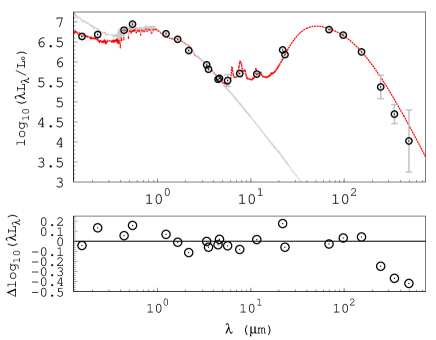
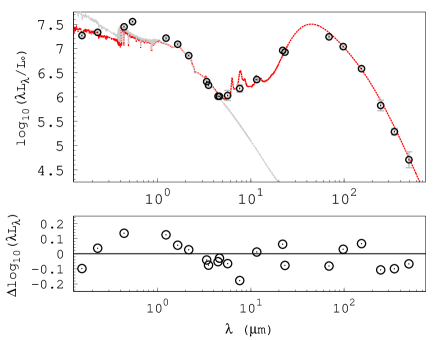
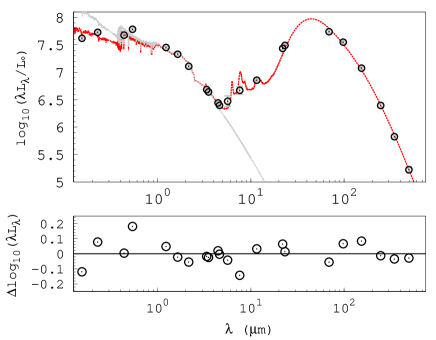
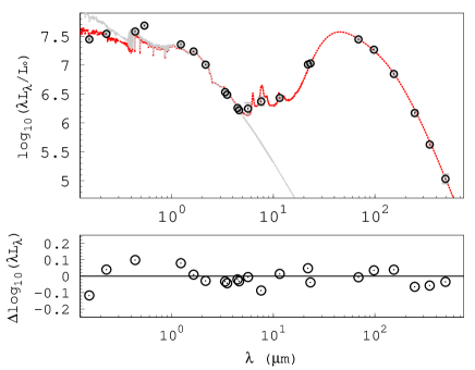
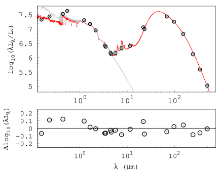
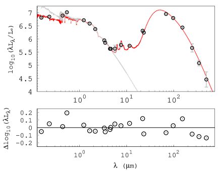
Figure 6: Best–fit model SEDs for the six pixels used to compare the two sets of convolved images. Here shown are the models using images convolved at the SPIRE 500 $\mu$m resolution (36.4$\arcsec$ FWHM), while the lower sub–panels show the residuals between the model and the observations. The middle left SED contains the cavity region and the SC 10, while North is to the left and East is to the bottom.

Fig. 6 shows the resulting best–fit model SEDs for the six pixels used in this comparison, at the SPIRE 500 $\mu$m resolution. As the pixels are large (42$\arcsec$), the cavity region with the SSCS, SC 10 and the bright north–western dust knot seen in Fig. 1 are all contained in one pixel. The corresponding SED to this pixel is shown in the middle left panel of Fig. 6, and the MIR and FIR emission there is brighter compared to the rest SEDs. The MIR emission drops in regions further from the SSCs.

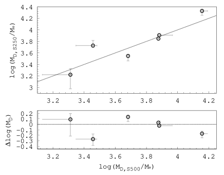
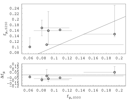
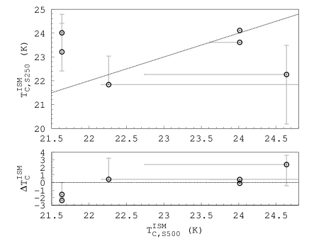
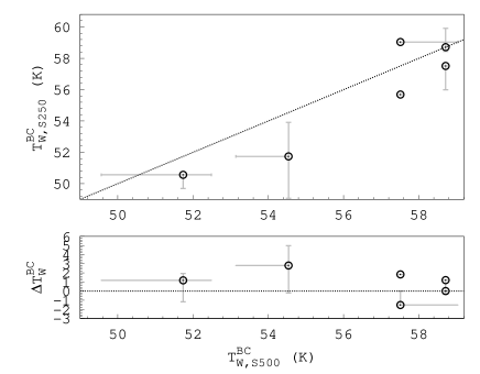
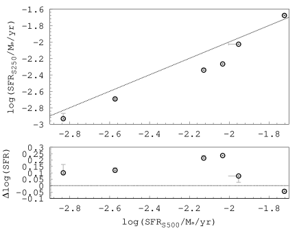
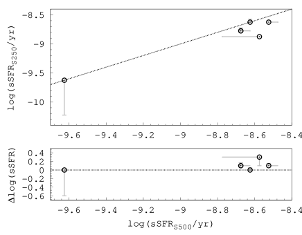
Figure 7: Physical parameters derived for the set of images convolved to the SPIRE 500 $\mu$m PSF (x–axis) and SPIRE 250 $\mu$m PSF (y–axis) and compared on a pixel–by–pixel basis with a pixel size of 42$\arcsec$. The physical parameters are the total dust mass, M_D, the fraction of the dust in the diffuse ISM versus the total dust mass, f$\mu$, the cold dust temperature in the diffuse ISM, T${}_{C}^{ISM}$, the warm dust temperature in the birth clouds, T${}_{W}^{BC}$, the star formation rate averaged over the last 100 Myr, SFR, and the specific SFR, sSFR. The lower panels show the difference of the physical parameter in the y–axis (i.e., at the SPIRE 250 $\mu$m resolution) and in the x–axis (i.e., at the SPIRE 500 $\mu$m resolution), $\Delta$(Physical Parameter), as a function of the one at the x–axis (i.e., at the SPIRE 500 $\mu$m resolution). The dotted line in the upper sub–panels indicate unity.

The results of the comparison between the median likelihood estimates of the physical parameters for the 2 sets of images are shown in Fig. 7. The error bars reflect the percentile ranges of the median likelihood estimates of the physical parameters, while the difference between these, $\Delta$(Physical Parameter), are shown in the lower sub-panels.

Fig. 7 suggests overall that the properties determined with the longest wavelength constraint being SPIRE 500 $\mu$m versus SPIRE 250 $\mu$m are consistent with each other, taking into account the uncertainties. The two parameters that seem to deviate the most are the f$\mu$ and T${}^{ISM}_{C}$. Decomposing the ISM into the different phases requires to take into account information from specific gas tracers, and this approach is lacking in the modelling technique used here. The standard deviation of the differences for the properties quoted above are: $\sigma_{\rm\Delta log(M_{D})}$= 0.16 dex; $\sigma_{\rm\Delta f_{\mu}}$= 0.05; $\sigma_{\rm\Delta T_{C}^{ISM}}$= 1.7 K; $\sigma_{\rm\Delta T_{W}^{BC}}$= 1.5 K; $\sigma_{\rm\Delta log(SFR)}$ = 0.1 dex; $\sigma_{\rm\Delta log(sSFR)}$ = 0.1 dex. The consistency between results with and without the SPIRE 350 & 500 $\mu$m data means that it is reasonable to use the latter for our quantitative analysis and thus gain in spatial resolution of 21$\arcsec$. The assumption of quiescent cold dust clumps not being taken into account in this modelling technique also points to data longwards to SPIRE 250 $\mu$m not needed. Moreover, a pixel size of 21$\arcsec$ points to the fact that within our pixels there is averaging of several different components of the ISM. For example, with a size for a giant molecular cloud of 100 pc, any cold ISM component will be well mixed with warmer regions. This means that our results may indicate warmer temperatures and smaller dust masses, as discussed in Sec. 6 and Sec. 7.

5 Properties on a pixel–by–pixel basis

In the pixel–by–pixel analysis, we focus on the parameters of M_D, f$\mu$, T${}_{C}^{ISM}$, T${}_{W}^{BC}$, SFR, and sSFR to see how these vary across the central starburst of NGC 1569. With a pixel size of 21 $\arcsec$ in the maps, the spatial scales probed are 294 pc on a side, i.e. larger than the size of the cavity (198 pc in diameter). The results obtained in this section are not used in subsequent sections to derive any new properties, and they are only used for comparison reasons.

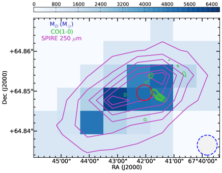
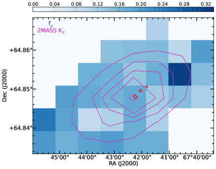
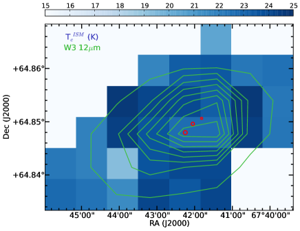
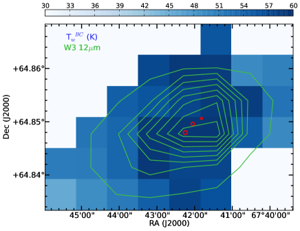
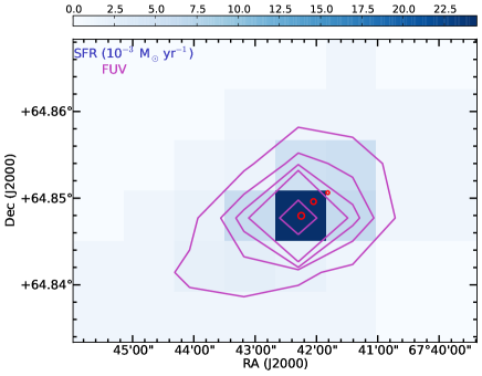
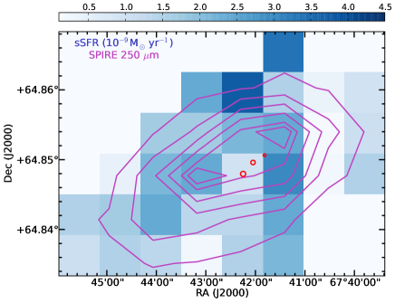
Figure 8: M_D, f$\mu$, T${}_{C}^{ISM}$, T${}_{W}^{BC}$, SFR, and sSFR maps at the SPIRE 250 $\mu$m resolution (18.2$\arcsec$ FWHM) and pixel scale 21$\arcsec$. Pixels with zero values have S / N ratio lower than the imposed cutoff. The contour levels are 1 Jy to 0.1 Jy with a step of 0.2 Jy for SPIRE 250$\mu$m, [100, 55, 40, 25, 10] mJy for K_S, and [90, 70, 35, 12.5, 8, 6, 3] mJy for FUV. The red solid circle in the M_D map shows the cavity, while in the remaining maps the small red circles show the location of the SSCs and SC 10. The blue dashed circle in the M_D map shows the size of the SPIRE 250 $\mu$m PSF.

The results on these parameters are shown in the maps of Fig. 8 and correspond to the median likelihood estimates for each parameter. The area of NGC 1569 covered in these maps is roughly 168$\arcsec\times$126$\arcsec$, while the true area is exactly 1.4$\times$10⁴ sq. arcsec (or 2.7 Mpc²; a total of 31 pixels), and is larger than the one shown in Fig. 2. The area of NGC 1569 covered in Fig. 8 corresponds to 37 per cent of its total area, which is 3.7$\times$10⁴ sq. arcsec (or 7.3 Mpc²) assuming a D₂₅ diameter of 216$\arcsec$. We are again restricted to pixels with S / N higher than 2 in the SPIRE 250 $\mu$m band. We discard pixels with S / N lower than that, and we flag these pixels’ properties with zero.

The upper left panel of Fig. 8 shows M_D, which ranges from 6.2${}^{+0.6}_{-1.2}$ to 1.0${}^{+0.3}_{-0.3}$ $\times$10 ³ M_⊙. The lower value, 1.0${}^{+0.3}_{-0.3}$ $\times$10 ³ M_⊙, in the outskirts corresponds to an upper limit, due to binning effects in the recorded probability density function of this parameter in magphys. The seemingly homogeneous distribution across the outer part of the galaxy’s mapped area hides the true variation in this parameter. At the central part of the galaxy, M_D fluctuates to higher values, with high amounts found in the periphery of the cavity, to the North–West and East from SSC A, and coinciding with the dust knots seen in the PACS and SPIRE bands. Given the large angular size of the pixels, the pixel west and northwest to the SSC A also includes the molecular clouds that are located in the periphery of the cavity (see upper left panel of Fig. 8; CO contours adapted from Taylor et al., 1999). On the other hand, the pixels to the East of SSC A contain several of the H ii regions studied in Waller (1991, see for example their Fig. 3b). Thus, the higher values of the M_D there reflect the embedded and ongoing star formation occurring in the molecular clouds and H ii regions (Waller, 1991; Taylor et al., 1999; Tokura et al., 2006). The pixel that contains SSC A and SSC B has a statistically lower value (M_D = 5.1${}^{+0.3}_{-0.6}$ $\times$10 ³ M_⊙) than its star-forming vicinity, as already noted in the earlier qualitative analysis of Sec. 3. This pixel probes the part of the cavity seen in both warm ionised and atomic hydrogen observations, but several other cavities in the ISM of smaller scale have been uncovered in the central part of the galaxy (e.g., Pasquali et al., 2011). These smaller scale cavities are smoothed out due to the relatively large angular resolution. The dust content around the SSCs and in the cavity is the subject of Sec. 7.

The total integrated M_D obtained from the dust mass map is 60.4${}^{+1.2}_{-3.5}$ $\times$ 10³ M_⊙. The M_D value is about an order of magnitude less than derived in Rémy-Ruyer et al. (2013, M_D= 2.8${}^{+1.5}_{-1.4}\times$10⁵ M_⊙), who consider modified blackbody fits to the dust SED in a circular aperture radius of 150$\arcsec$, and than derived in Galliano et al. (2003, M_D= (1.6–3.4)$\times$10⁵ M_⊙), who consider a detailed dust model for the galaxy within a radius of 0.65 kpc. The area of the galaxy used to model the SEDs between this work and the works of Rémy-Ruyer et al. (2013) and Galliano et al. (2003) is different, thus the derived M_D refer to different regions of the galaxy, to begin with. Dividing our dust mass by the area probed, i.e. 1.4$\times$10⁴ sq. arcsec, we derive 2.3${}^{+1.2}_{-0.7}$ $\times$ 10⁴ M_⊙ kpc^-2. Normalising the dust mass found in Rémy-Ruyer et al. (2013) by their considered area, i.e. 7.1$\times$10⁴ sq. arcsec, we derive 2.0${}^{+1.1}_{-1.0}$ $\times$ 10⁴ M_⊙ kpc^-2. The two dust mass density values are consistent within the uncertainties. As NGC 1569 has extended emission in the warm and cold ISM components, averaging the dust mass over the area probed is meaningful out to distances where such an extended emission is seen. Fig. 4 implies that the extended emission goes beyond 180$\arcsec$.

Comparing with the results of Galliano et al. (2003), we normalise their dust mass by their considered area, i.e. 1.5 kpc², to derive a dust mass density of (1.1–2.3) $\times$ 10⁵ M_⊙ kpc^-2. This is a larger dust mass per unit area than what we derive here, larger by a factor of $\sim$7. The difference in the two dust mass density values can be further understood as due to the differences in the modelling techniques between these works. Indeed, Galliano et al. (2003) develop a detailed dust model to derive the dust grain properties, such as grain size distribution, and dust masses. Their modelling assumptions and approach are different from the ones in magphys, which give rise to differences in the derived dust masses. Galliano et al. (2003) include a very cold grain component in their model, in order to fit the excess emission in the millimetre wavelength range. They model this very cold grain component with a modified blackbody with fixed $\beta$ of 1, and they find that 40 per cent to 70 per cent of the cold dust mass resides in this very cold grain component.

The source of heating for the diffuse ISM is the old and intermediate age stars with ages larger than 10 Myr. The upper right panel of Fig. 8 shows the distribution of f_μ in the central part of NGC 1569, which ranges from 0.31$\pm$0.01 to 0.09${}^{+0.02}_{-0.01}$. The spatial distribution of f_μ is consistent with a homogeneous distribution. We would expect the diffuse ISM in the very central starburst to be negligible as compared to the denser phases in the same region. The pixel that contains the two SSCs has f_μ of 0.17${}^{+0.01}_{-0.01}$. The overlaid K_S contours show a homogeneous distribution of the stellar mass in the galaxy, as also found for the distribution of the intermediate–age (50 Myr to 1 Gyr) and old resolved stellar populations (with ages larger than 1 Gyr; Aloisi et al., 2001).

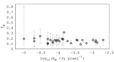
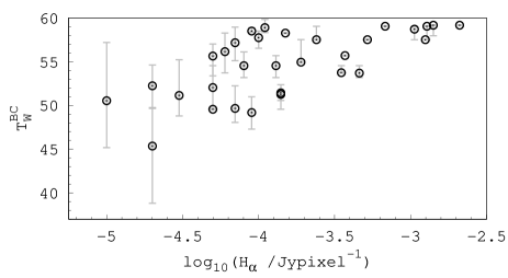
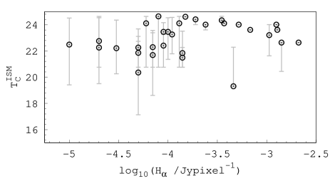
Figure 9: Derived properties with magphys versus observed properties.

Fig. 9 shows f_μ as a function of the H $\alpha$ flux density, per pixel. The two quantities show no correlation. As stars younger than 10 Myr contribute to the H $\alpha$ emission, the lack of correlation may indicate that the diffuse ISM is heated by stars with ages larger than those traced with H $\alpha$. Alternatively, the spatial distribution of stars with ages younger than 10 Myr is different than those with older ages, consistent with the findings of Aloisi et al. (2001).

da Cunha et al. (2008) consider in their model warm and cold grains in thermal equilibrium. The warm grains in thermal equilibrium reside in the diffuse ISM, characterised by a temperature T${}_{W}^{ISM}$, and in the birth clouds, characterised by a temperature T${}_{W}^{BC}$. The cold grains in thermal equilibrium reside in the diffuse ISM and are characterised by a temperature T${}_{C}^{ISM}$. da Cunha et al. (2008) fix T${}_{W}^{ISM}$ to 45 K, and adopt an emissivity index $\beta$ = 1.5 for the warm grains in the birth clouds, and $\beta$ = 2 for the cold dust in the diffuse ISM. The thermal equilibrium temperatures are shown in the middle left and right panels of Fig. 8, for the cold dust in the diffuse ISM and for the warm dust temperature in the birth clouds, respectively. These parameters are allowed to vary between 15 K to 25 K for the cold dust, and between 30 K to 60 K for the warm dust in the birth clouds. The range mapped in T_C is from 19.3${}^{+3.0}_{-1.0}$ K to 24.6${}^{+0.4}_{-3.9}$ K, while the T_W map ranges from 45.4${}^{+4.4}_{-6.5}$ K to 59.2${}^{+0.6}_{-1.2}$ K. The lowest T_C is located roughly southeast of the cavity, where dense H i clouds are also found (Johnson et al., 2012, their Fig. 18). The PAH–sensitive emission, indicated with the W3 12$\mu$m contours, shows that brighter emission is associated with colder equilibrium temperature in the diffuse ISM and warmer equilibrium temperature in the BCs. Fig. 9 shows T${}_{W}^{BC}$ and T${}_{C}^{ISM}$ as a function of the H $\alpha$ flux density per pixel. The pixels with warmer dust in the birth clouds have higher H $\alpha$ emission, while the pixels with colder dust show no correlation with stars younger than 10 Myr.

The SFR in magphys is derived from the stellar population synthesis component of the SED, and is averaged over the past 100 Myr. Thus, it is tied to the stellar emission directly, rather than the dust emission. The SFR, shown in the lower left panel of Fig. 8 ranges from 1.0${}^{+0.2}_{-0.1}$ $\times$10 ^-3 to 24.4${}^{+1.0}_{-11.0}$ $\times$10 ^-3 M_⊙ yr^-1. The lower value, 1.0${}^{+0.2}_{-0.1}$ $\times$10 ^-3 M_⊙ yr^-1, in the outskirts corresponds to an upper limit, due to binning effects in the recorded probability density function of this parameter in magphys. The highest SFR is found in the pixel that contains SSC A, which reflects the massive star formation that occurs in the form of the SSCs. The integrated SFR in the central part of the galaxy is 76.8${}^{+0.4}_{-0.1}$ $\times$10 ^-3 M_⊙ yr^-1. Hunter et al. (2010) find a SFR_FUV of 13.8 ($\pm$0.0) $\times$10 ^-2 M_⊙ yr^-1, and a SFR_Hα of 12.6 ($\pm$0.0) $\times$10 ^-2 M_⊙ yr^-1, while McQuinn et al. (2012, their Table 1) find a SFR_SFH of 76$\pm$2 $\times$10 ^-3 M_⊙ yr^-1. All these results compare well with our derived value, which is limited to the very central region of the galaxy.

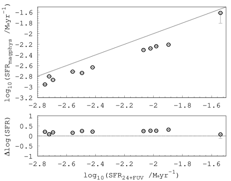
Figure 10: SFR (median likelihood) derived with magphys versus SFR_24+FUV. The lower panel shows their difference in the sense SFR${}_{24+FUV}-$SFR_magphys.

Fig. 10 compares the SFR derived with magphys and the one derived from the combination of FUV and 24 $\mu$m (Leroy et al., 2008). We do not correct for effects of the old stellar population (Ford et al., 2013), as the central region studied here is dominated by the starburst (Aloisi et al., 2001). When we compute the SFR from the combination of FUV and 24 $\mu$m, we correct the FUV for internal extinction by a factor of 2.63, corresponding to the average optical extinction found by Pasquali et al. (2011, $\langle$A${}_{V}\rangle$ = 0.40 mag). The pixel–by–pixel comparison between the two tracers in Fig. 10 shows that the SFR derived with magphys is lower than the one derived with the combination of FUV and 24 $\mu$m, with a mean difference of 0.2 $\pm$ 0.1 dex. Viaene et al. (2014) also report a similar offset in their comparison of the same two SFRs, and attribute the difference to the different way these SFR tracers are derived. The SFR based on the combination of FUV and 24 $\mu$m is calibrated for much more massive galaxies and on global scales, while the SFR derived with magphys here refers to local scales within a low-mass dwarf galaxy.

The sSFR map is shown in Fig. 8 with values ranging between 0.2${}^{+0.1}_{-0.1}$ $\times$10 ^-9 yr^-1 and 3.8${}^{+1.3}_{-3.9}$ $\times$10 ^-9 yr^-1. The sSFR is higher in the periphery of the cavity. The sSFR map shows that this physical property is more sensitive to the details of the local star formation in the periphery of the cavity. The sSFR variations is driven by the stellar mass variations, which are highest in the central region of the cavity and SSCs.

6 Gas–to–dust mass ratio

In order to derive the gas–to–dust (G/D) mass ratio on a pixel–by–pixel basis, we use the dust masses from Sec. 5 (the pixel–by–pixel analysis) and the total gas mass, which we derive in what follows. There are three gas components present in NGC 1569: the atomic hydrogen; the warm ionised hydrogen; and the molecular hydrogen. Literature values give an atomic hydrogen mass of 2.5$\times$10⁸ M_⊙ (Hunter et al., 2012), a warm ionised gas of 1.3$\times$10⁵ M_⊙ (Hunter et al., 2010), and a CO–traced molecular gas mass of 2$\times$10⁶ M_⊙ (Greve et al., 1996; Taylor et al., 1999).

Both the H i and H $\alpha$ morphology of NGC 1569 shows extended emission beyond the optical body of the galaxy, as well as cavities within. On the other hand, the CO morphology shows emission concentrated primarily in the west and to a lesser degree in the southeast to the cavity with no detectable contributions elsewhere (Greve et al., 1996), and most of this emission is in the form of giant molecular clouds located in the west and northwest of the cavity (Taylor et al., 1999). The interferometric observations of Taylor et al. (1999) may have missed any diffuse CO emission present. Thus, the warm ionised and atomic hydrogen gas are expected to have equally low contributions within the cavity, while elsewhere the atomic hydrogen should dominate by mass. The CO–derived molecular hydrogen is expected to contribute significantly in the northwest and west of the cavity, while elsewhere the atomic hydrogen mass should dominate.

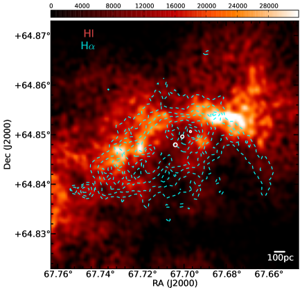
Figure 11: H i map within 180$\arcsec\times$180$\arcsec$, with contours of H $\alpha$ overlaid in dashed cyan, as in Fig. 4. The white solid circles indicate the location of the SSCs and SC 10. The units of the map are mJy / pixel $\times$ km / sec.

To obtain the atomic hydrogen mass on a pixel–by–pixel basis, we use the Very Large Array (VLA) data set presented in LITTLE THINGS by Hunter et al. (2012) and retrieved from NRAO. We use their primary–beam–corrected moment 0 map, shown in Fig. 11, in conjunction with the equation:

$$M_{\mbox{H\,{\sc i}}}\,({\rm M_{\odot}})=235.6\,D^{2}\sum(S\,\Delta V)$$ (2)

where M${}_{\mbox{H\,{\sc i}}}$ is the atomic hydrogen mass, $D$ is the distance of NGC 1569 in Mpc, $S$ is the H i flux density in mJy, integrated along the velocity axis, $\Delta V$ (2.6 km sec^-1).

To obtain the warm ionised hydrogen mass on a pixel–by–pixel basis, we use the H $\alpha$ map (stellar continuum and background corrected) from Hunter & Elmegreen (2006), in conjunction with eq. 10 in Kulkarni et al. (2014, see also ):

$$M_{\rm H\alpha}\,({\rm M_{\odot}})=2.33\times 10^{3}\left(\frac{L_{\rm H\alpha}}{10^{39}}\right)\left(\frac{10^{3}}{n_{e}}\right)$$ (3)

where M_Hα is the warm ionised gas mass, L_Hα is the H$\alpha$ luminosity (erg/sec), and n_e the electron density, assumed equal to 10³ cm^-3.

The molecular hydrogen mass is usually traced through CO observations, assuming a conversion factor between them, which depends on the metallicity and is thus largely uncertain (Wilson, 1995; Rémy-Ruyer et al., 2014). Additionally, Madden et al. (2013) and Cormier et al. (2014) discuss that CO is a poor tracer of molecular hydrogen gas in low–metallicity dwarf galaxies, while the [C ii] 158 $\mu$m fine-structure line becomes a better tracer and provides better insights on the presence of the molecular gas component. NGC 1569 is more luminous in [C ii] than CO, with luminosity ratio L${}_{\mbox{[C\,{\sc ii}]}}$ / L_CO of 3.7$\times$10⁴ (Hunter et al., 2001), and further modelling of the line strengths of forbidden lines suggests a molecular gas mass of 3.2$\times$10⁷ M_⊙ (Hunter et al., 2001, their Table 6), i.e. 13 per cent of the atomic hydrogen mass.

Here, we use the CO observations from Taylor et al. (1999) to include the molecular gas mass in our analysis, as follows. The contribution from the CO-traced molecular gas is in the 5 giant molecular clouds, each of which with masses listed in Table 3 of Taylor et al. (1999). The giant molecular clouds designated with numbers 1,2, & 3 in Taylor et al. (1999) are located in one pixel, west of SSC A (see Fig. 8), and have a total molecular gas mass of (multiplied by a factor of 1.8 to correct for the distance adopted here) 26.1($\pm$4)$\times$10⁵ M_⊙. We add this mass to the total gas mass in the pixel west of SSC A. The giant molecular clouds designated with numbers 4 & 5 in Taylor et al. (1999) are located in two pixels, north and northwest of SSC A (see Fig. 8), and have a total molecular gas mass of 3.9($\pm$0.7)$\times$10⁵ M_⊙ (corrected for our adopted distance). We divide this amount of mass to the total gas mass in the two pixels, north and northwest to the SSC A.

The conversion factor between CO and H₂ used in Taylor et al. (1999, their Table 3) is modified from the Galactic value using the virial theorem, with an average value of 6.6$\pm$1.5 times that of the galactic value. As discussed in Schruba et al. (2012), using the virial theorem to derive the conversion factor may lead to underestimated values for the molecular gas mass. These authors assume a constant star formation efficiency to derive a functional form for the metallicity dependence of the conversion factor for a sample of dwarf galaxies. Using the relation between the metallicity and the conversion factor derived for their whole HERACLES sample (see Table 7 in Schruba et al., 2012), and assuming a gas phase metallicity of 8.02$\pm$0.02 (Madden et al., 2013), the conversion factor is 183${}^{+137}_{-77}$ M_⊙ pc${}^{-2}($K km s${}^{-1})^{-1}$, and the ratio of this with the Galactic conversion factor is 42${}^{+31}_{-18}$. Comparing this ratio with the average ratio 6.6$\pm$1.5 of Taylor et al. (1999) indicates that the total molecular gas mass in the giant molecular clouds, which we use in this study, may have been underestimated by a factor of $\sim$6, leading to an even higher total gas mass, as well as a higher G / D mass ratio in those pixels that contain the giant molecular clouds considered here.

The total gas mass is the sum of all gas components. We also consider the helium gas and the gaseous metals, thus the total gas mass is expressed as (see eq. 3 in Rémy-Ruyer et al., 2014):

$$M_{gas}=1.38\times(M_{\mbox{H\,{\sc i}}}+M_{\rm H_{2}}+M_{\rm H\alpha})$$ (4)

where M${}_{\mbox{H\,{\sc i}}}$ is the atomic hydrogen mass, M${}_{\rm H_{2}}$ is the molecular hydrogen mass, and M${}_{\rm H\,\alpha}$ is the warm ionised hydrogen mass. The 1.38 factor includes the contribution from the helium gas and the gaseous metals. Before summing up the individual gas components, we process the maps in the same way as described in Sec. 2, i.e. convolving these to the SPIRE 250 $\mu$m PSF and re-sampling to a 21$\arcsec$ pixel size, in accord with the dust mass maps shown in Fig. 8.

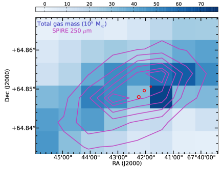
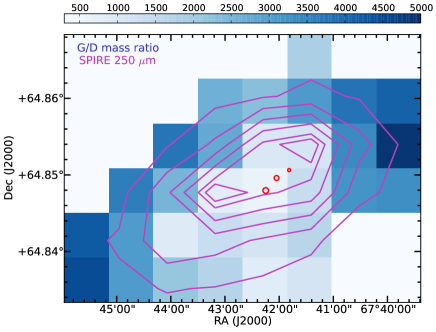
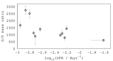
Figure 12: Total gas mass map (upper panel), G/D mass ratio map (middle panel), and G/D mass ratio versus SFR based on the magphys modelling (lower panel).

The resulting total gas mass map for the same central region as the dust mass map (shown in Fig. 8) is shown in the upper panel of Fig. 12. We obtain ranges for the total gas mass between 0.27($\pm$0.03) $\times$ 10⁶ M_⊙ to 7.10($\pm$0.39) $\times$ 10⁶ M_⊙. The total gas mass increases towards the periphery of the cavity, with the maximum mass observed west of SSC A. The cavity and SSCs region has a total gas mass of 3.1($\pm$0.3)$\times$10⁶ M_⊙, primarily driven by the atomic gas component. The size of the pixel (21$\arcsec$) is large enough to include atomic hydrogen emission from the vicinity of the cavity (see Fig. 11).

We use the dust mass on a pixel–by–pixel basis derived in Sec. 5 to get the G/D mass ratio variation in the central starburst region of NGC 1569, shown in the middle panel of Fig. 12. We obtain G/D mass ratio ranging between 0.60${}^{+0.07}_{-0.10}$ $\times$ 10³ to 4.88${}^{+0.54}_{-0.54}$ $\times$ 10³. The G/D mass ratio becomes larger beyond the periphery of the cavity, where the total gas mass dominates over the dust mass, showing the gas–rich nature of the galaxy as seen in the H i map in Fig. 11. The variation of the G/D mass ratio in the very central starburst is driven by the variation of the dust mass there, which is larger than the outer parts (see also the dust mass map in Fig. 8). The G/D mass ratio has the smallest value in the cavity and SSCs region, primarily driven by the total gas mass there. At the location of the cavity, the total gas decreases due to the decrease of the atomic hydrogen gas, as seen in the H i map in Fig. 11 and in the total gas map in Fig. 12 (upper panel).

Kobulnicky & Skillman (1997) report that NGC 1569 doesn’t show any significant oxygen abundance gradient, which they limit to less than 0.05 dex per kpc. The G/D mass ratio shows a dependence on metallicity (Rémy-Ruyer et al., 2014; Sandstrom et al., 2013, and references therein), and, due to the flat abundance gradient in NGC 1569, the G/D mass ratio would be expected to remain constant. The preceding paragraph discusses how the variation of the total gas and of the dust mass drives the variation of the G/D mass ratio in NGC 1569 across the central starburst. Moreover, an additional component of quiescent cold dust clumps, which is not included in the modelling here, could drive the dust masses in the outer parts to larger values, and thus reconcile the G/D mass ratio to a constant value across the dwarf galaxy. Assuming an average total gas mass per pixel of $\sim$3$\times$10⁶ M_⊙ and an average G/D mass ratio per pixel of $\sim$1000 yields an average dust mass of $\sim$3$\times$10³ M_⊙ per pixel. Thus, about 2$\times$10³ M_⊙ of dust mass larger than what inferred with the dust modelling, per pixel. Assuming an average size of 300 pc per pixel, this translates to $\sim$7 M_⊙ per pc of dust mass needed in quiescent cold dust clumps. For comparison, Rathborne et al. (2010, their Table 5) derive dust masses of $\sim$50 M_⊙ per pc for quiescent clump cores in Galactic infrared-dark clouds, with the latter harbouring the earliest phases of star cluster formation (Rathborne et al., 2006). Whether such quiescent cold dust clumps exist in NGC 1569 remains to be uncovered.

The integrated G/D mass ratio in the central starburst region results to 75.5(${}^{+1.8}_{-1.9})$ $\times$ 10³. Such large G/D mass ratios are also observed in other low–metallicity dwarf galaxies (Rémy-Ruyer et al., 2014). The lower panel of Fig. 12 shows the G/D mass ratio as a function of the SFR, per pixel, derived from the magphys modelling in Sec. 5. There is a trend of regions with higher SFRs to have smaller G/D mass ratio, consistent with what is expected in terms of gas fuelling star formation. The highest SFR is observed in the cavity region, associated with the SSCs, and there is where the lowest G/D mass ratio is also observed. In the periphery of the cavity there is embedded and ongoing star formation, and there the G/D mass ratio is lower compared to the outer parts. In the outer parts, the SFR is low, while the G/D mass ratio is large.

7 Cavity and SSCs

The winds from the SSCs have impacted the ISM around them by creating the cavity seen in warm ionised and atomic hydrogen observations. While the angular resolution of our images does not allow us to zoom into the properties of the SSCs, the set of convolved images at the SPIRE 250 $\mu$m PSF allows us to study the cavity region. It is thus interesting to compare the star and dust properties of the cavity versus the central starburst, as a way to understand the impact of the SSCs on the surrounding ISM. For this analysis, we model the SED anew for the cavity and the central starburst region.

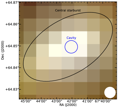
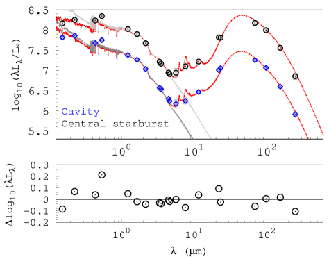
Figure 13: Left panel: The apertures used for the new SED modelling of the cavity (blue circle) and the central starburst (black ellipse) are overlaid on a three colour image of the galaxy composed of SPIRE 250 $\mu$m in red, PACS 100 $\mu$m in green, and W3 12 $\mu$m in blue. The field-of-view covered is 180$\arcsec$ on a side, with a pixel size 21 $\arcsec$. The images are convolved to the SPIRE 250 $\mu$m PSF, which is shown as the white circle on the right bottom. Right panel: Modelled (best–fit) and observed SED for the cavity and the central starburst at the SPIRE 250 $\mu$m resolution. The red (darker) curves show the attenuated modelled spectrum, while the grey (lighter) curves show the unattenuated spectrum. Black circles correspond to the central starburst observed spectral luminosity, and blue diamonds to the cavity region one. The lower sub-panel shows with black circles the difference of the observed and modelled SED for the central starburst region.

For the central starburst, we construct its SED summing the pixels within an ellipse of semi–major axis 82$\arcsec$, major–to–minor axis ratio of 0.55, and position angle of 31^∘, centred on the galaxy. The choice of this ellipse area is to maximise the area that contains pixels with S / N higher than the imposed cutoff. The semi–major axis used corresponds to 76 per cent the D₂₅ radius (216$\arcsec$). The ellipse encloses an area of 1.1$\times$10⁴ sq. arcsec, which is 31 per cent of the total galaxy area. The apertures used for the cavity and the central starburst are shown overlaid in the three–colour image of Fig. 13. The right panel in Fig. 13 shows the observed and (best–fit) modelled SEDs for the cavity and the central starburst.

Table 4: SED modelling results for the cavity and central starburst regions, using the set of images convolved to the SPIRE 250 $\mu$m PSF and with a 21$\arcsec$ pixel size.

Property	Cavity	Central starburst
RA (J2 000.0)	4 30 48.19	4 30 49.0
Dec (J2 000.0)	64 50 58.6	64 50 53
LD (108 L⊙)	0.40${}^{+0.02}_{-0.02}$	3.10${}^{+0.02}_{-0.04}$
MD (104 M⊙)	0.5${}^{+0.1}_{-0.1}$	4.3${}^{+1.2}_{-0.6}$
T${}_{C}^{ISM}$ (K)	22.6${}^{+1.1}_{-1.1}$	24.0${}^{+0.2}_{-0.4}$
T${}_{W}^{ISM}$ (K)	59.2${}^{+0.6}_{-1.2}$	59.0${}^{+0.8}_{-1.5}$
SFR (10-2 M⊙ yr-1)	2.52${}^{+0.01}_{-0.01}$	5.78${}^{+0.04}_{-0.07}$
sSFR (10-9 yr-1)	0.9${}^{+0.5}_{-0.5}$	2.4${}^{+0.3}_{-0.3}$

Table 4 summarises the results on the derived properties (median likelihood estimates) for the cavity and central starburst from this new SED modelling with magphys. These results show that the cavity region contains 13 per cent the L_D and 12 per cent the M_D of the central starburst region. The SFR and sSFR of the cavity are $\sim$40 per cent that of the central starburst region, signifying the massive star formation in the SSCs. The equilibrium temperatures are statistically equivalent between the cavity and the central starburst region.

The values listed in Table 4 are the result of modelling anew the SEDs of these regions, and are not obtained by summing up the star and dust properties derived in the pixel–by–pixel analysis of Sec. 5. To compare between the (summed–up) properties derived in Sec. 5 and the properties listed in Table 4, we first normalise each by the area probed.

Table 5: Normalised by area properties obtained in this section and in Sec. 5 for the central starburst region.

Properties	This section	Sec. 5
LD (108 L⊙ kpc-1)	1.38${}^{+0.02}_{-0.04}$	1.68${}^{+0.35}_{-0.60}$
MD (104 M⊙ kpc-1)	1.9${}^{+1.2}_{-0.6}$	2.3${}^{+1.2}_{-0.7}$
SFR (10-2 M⊙ yr-1 kpc-1)	2.57${}^{+0.04}_{-0.07}$	2.87${}^{+0.04}_{-0.07}$
sSFR (10-8 yr-1 kpc-1)	0.1${}^{+0.3}_{-0.3}$	1.9${}^{+0.3}_{-0.6}$

The area–normalised properties are listed in Table 5. This comparison shows that the normalised properties for the central starburst region are consistent with each other, with the exception of the sSFR. The sSFR is higher by an order of magnitude in the case of summing up the sSFR found in each pixel in Sec. 5. The area enclosed in the latter case is larger than the one we use in this section. The sSFR depends on the inverse of the stellar mass, by definition, and the stellar mass is not constant as a function of radius, thus the difference between the two sSFR.

As the central starburst region covers a smaller area than that of the whole galaxy, this implies that the fractional dust mass in the cavity versus the whole galaxy is even lower. Galliano et al. (2011) find that there is a bias introduced on deriving dust masses according to the spatial resolution probed, i.e., summing up the dust mass on pixel sizes of various spatial resolutions within the LMC versus integrating over a larger area to derive its dust mass results in underestimating the dust mass in the latter case. They find an optimal spatial scale of $\sim$30–50 pc for the LMC, for which the dust mass estimates become stable over the chosen spatial scale. We cannot probe such small spatial scales. Comparing the spatial scales we probe here for the cavity (and in Sec. 5; pixel size of 21$\arcsec$ or 294 pc) with Fig. 6 in Galliano et al. (2011, lower panels), the dust mass estimate of the LMC at our spatial resolution is roughly in accord with the one at their optimal spatial resolution element, within the uncertainties. For the central starburst region in this section (spatial scale of 1.2 kpc in diameter), the findings of Galliano et al. (2011) indicate that the dust mass we derive may be underestimated as compared to deriving the dust mass in a finer resolution spatial scale, thus the dust mass we derive here for the central starburst may be considered as a lower limit. All these point to a stronger case of the dust mass within the cavity being a small fraction of that of the central starburst, and further implying that it is even lower than that. This is consistent with the finding of Sec. 3 on the dust emission morphology.

It is interesting to place our findings on the dust content in NGC 1569’s cavity in the wider context of galaxy evolution and Galactic GCs. Our analysis shows that the dust luminosity and dust mass in the cavity region is low compared to the galaxy’s central starburst dust content. The low levels of dust emission in the cavity region compared to the central starburst is in accord with the disrupted nature of the cavity region initially seen in the warm ionised and atomic hydrogen phase. All phases of the ISM thus far studied (warm and hot ionised gas, atomic hydrogen gas, CO–traced molecular hydrogen gas, dust emission) show a deficit of emission in the cavity. The ISM structure in the cavity is a result of the massive starburst, which gave rise to SSC winds and created superbubble kinematics and galactic scale outflows further driving the ISM evolution (Westmoquette et al., 2008; Martin, 1998).

Even though the SSCs have affected the ISM in the central starburst region of the dwarf galaxy and may have caused the galactic–scale outflows, these have not affected the morphology of the atomic hydrogen gas on global scales or ceased star formation (see also discussion in Holwerda et al., 2013). On the contrary, dust knots and ongoing star formation activity is observed in the periphery of the cavity, while the SED modelling implies the need of quiescent cold dust clumps so as to reconcile the G/D mass ratio with an observed flat metallicity gradient (Kobulnicky & Skillman, 1997; Devost et al., 1997). It would require either additional mechanisms external to the galaxy (see, for example, Lianou & et al., 2013b) to completely remove the ISM, or subsequent bursts of massive star formation distributed across the whole body of the galaxy and with intensity similar to the one produced by the SSCs, in order to clear out the ISM in their vicinity. Bagetakos et al. (2011) study the distribution of H i holes in a large sample of galaxies and find that those in dwarf galaxies extend beyond their R₂₅ radius. With a stellar mass of 2.8$\times$10⁸ M_☉, the feedback from the current massive star formation alone is not enough to affect the atomic hydrogen on global scales in this dwarf galaxy or to cease the star formation activity in the periphery of the cavity and beyond.

The two SSCs reside within the cavity region and are at an earlier evolutionary phase as compared to their likely old counterparts, i.e. the old massive GCs (de Grijs et al., 2005). The majority of the studied Galactic GCs are found to be devoid of dust, which is unexpected considering evolutionary effects on their stellar population (Barmby et al., 2009; Priestley et al., 2011). The evolution of GCs is affected by the geometry and mass of their host galaxy (e.g., Madrid et al., 2014). NGC 1569 offers a simpler environment than the one in the Galaxy, free from spiral structure, albeit with a complex and disturbed ISM. Assuming the SSCs as the likely progeny of the old GCs seen in our Galaxy, the former possess a low dust content already early in their life, before any complex processes due to the galactic geometry having affected their evolution.

8 Summary & conclusions

We use a multiwavelength data set from UV to submm to construct the observed SEDs of the central region of NGC 1569. We model the observed SEDs with magphys on a pixel–by–pixel basis, as well as the cavity and central starburst regions of the galaxy. We investigate whether the derived physical parameters depend on the choice of which bands to retain for the SED fitting. Results obtained without using the SPIRE 350 $\mu$m and 500 $\mu$m bands are consistent with results obtained using those bands. We perform our analysis using images at the SPIRE 250 $\mu$m resolution, in order to gain in spatial resolution. We show the variation of the derived properties on a pixel–by–pixel basis and focus on the cavity region versus the central starburst. We derive the total gas mass, considering the warm ionised, atomic and CO–traced molecular hydrogen gas, and investigate its variation as a function of the dust mass on a pixel–by–pixel basis and for the cavity and central starburst regions of the galaxy.

Our results are summarised as follows:

• The morphology of the central starburst region of the dwarf galaxy shows low levels of dust emission in the cavity region, as well as several dust knots marking the periphery of the cavity (Fig. 1). The brightest of the dust knots resolved in most of the Herschel bands is associated with the onset of an H $\alpha$ filament to the west and northwest of SSC A (Fig. 1 and Fig. 4).

• The extended emission seen in the warm and hot ionised gas is also seen in the warm and cold dust. All these components of the extended emission spatially correlate, while the emission probed with Herschel is more extended (Fig. 4 and Fig. 5).

• The dust content within the cavity region is low (12 per cent) compared to the central starburst region (Table 4 and Fig. 2). The spatial variation of the dust mass shows enhanced dust masses in the periphery of the cavity (Fig. 8). All tracers of the ISM thus far studied show the same picture of the cavity having low emission as compared to its vicinity or central starburst (Fig. 8, Fig. 11, and Fig. 12).

• The G/D mass ratio is higher in the periphery of the cavity compared to that of the cavity itself (Fig. 12).

The evolution of NGC 1569 has been affected by an interaction event (Stil & Israel, 1998; Jackson et al., 2011; Johnson, 2013), which has triggered the massive starburst (Angeretti et al., 2005; Anders et al., 2004; Hunter et al., 2000). The massive starburst has affected the surrounding ISM through stellar cluster winds and the ISM there is faint in dust, atomic hydrogen, and warm ionised hydrogen emission. The ISM further presents galactic scale outflows and extended emission beyond the optical body (Westmoquette et al., 2008; Martin, 1998; Heckman et al., 1995). External (i.e., galaxy interactions) and internal (i.e., SSC feedback) mechanisms are linked into driving the dwarf galaxy’s evolution. Within this context, dwarf galaxies displaying a starburst nature are now showing evidence of gravitational interactions with a lower-mass satellite companion causing the starburst and peculiar kinematics (e.g., Martínez-Delgado et al., 2012).

References

- Aloisi et al. (2001) Aloisi A., Clampin M., Diolaiti E., et al. 2001, AJ, 121, 1425
- Anders et al. (2004) Anders P., de Grijs R., Fritze-v. Alvensleben U., Bissantz N., 2004, MNRAS, 347, 17
- Angeretti et al. (2005) Angeretti L., Tosi M., Greggio L., et al. 2005, AJ, 129, 2203
- Aniano et al. (2012) Aniano G., Draine B. T., Calzetti D., et al. 2012, ApJ, 756, 138
- Aniano et al. (2011) Aniano G., Draine B. T., Gordon K. D., Sandstrom K., 2011, PASP, 123, 1218
- Astropy Collaboration et al. (2013) Astropy Collaboration Robitaille T. P., Tollerud E. J., et al. 2013, A&A, 558, A33
- Baes et al. (2010) Baes M., Fritz J., Gadotti D. A., et al. 2010, A&A, 518, L39
- Bagetakos et al. (2011) Bagetakos I., Brinks E., Walter F., et al. 2011, AJ, 141, 23
- Barmby et al. (2009) Barmby P., Boyer M. L., Woodward C. E., et al. 2009, AJ, 137, 207
- Bendo et al. (2012) Bendo G. J., Galliano F., Madden S. C., 2012, MNRAS, 423, 197
- Benson et al. (2003) Benson A. J., Bower R. G., Frenk C. S., et al. 2003, ApJ, 599, 38
- Bertin & Arnouts (1996) Bertin E., Arnouts S., 1996, A&AS, 117, 393
- Besla et al. (2012) Besla G., Kallivayalil N., Hernquist L., et al. 2012, MNRAS, 421, 2109
- Bianchi & Xilouris (2011) Bianchi S., Xilouris E. M., 2011, A&A, 531, L11
- Billett et al. (2002) Billett O. H., Hunter D. A., Elmegreen B. G., 2002, AJ, 123, 1454
- Bitsakis et al. (2014) Bitsakis T., Charmandaris V., Appleton P. N., et al. 2014, A&A, 565, A25
- Bitsakis et al. (2011) Bitsakis T., Charmandaris V., da Cunha E., et al. 2011, A&A, 533, A142
- Bolatto et al. (2013) Bolatto A. D., Warren S. R., Leroy A. K., et al. 2013, Nature, 499, 450
- Boomsma et al. (2005) Boomsma R., Oosterloo T. A., Fraternali F., van der Hulst J. M., Sancisi R., 2005, A&A, 431, 65
- Bruzual & Charlot (2003) Bruzual G., Charlot S., 2003, MNRAS, 344, 1000
- Burstein & Heiles (1982) Burstein D., Heiles C., 1982, AJ, 87, 1165
- Calzetti (2013) Calzetti D., 2013, Star Formation Rate Indicators. p. 419
- Calzetti et al. (1996) Calzetti D., Kinney A. L., Storchi-Bergmann T., 1996, ApJ, 458, 132
- Cesarsky et al. (1996) Cesarsky D., Lequeux J., Abergel A., et al. 1996, A&A, 315, L305
- Charlot & Fall (2000) Charlot S., Fall S. M., 2000, ApJ, 539, 718
- Clark et al. (2013) Clark D. M., Eikenberry S. S., Raines S. N., et al. 2013, MNRAS, 428, 2290
- Cormier et al. (2014) Cormier D., Madden S. C., Lebouteiller V., et al. 2014, A&A, 564, A121
- da Cunha et al. (2008) da Cunha E., Charlot S., Elbaz D., 2008, MNRAS, 388, 1595
- da Cunha & et al. (2010a) da Cunha E., et al. 2010a, A&A, 523, A78
- da Cunha & et al. (2010b) da Cunha E., et al. 2010b, MNRAS, 403, 1894
- de Grijs et al. (2005) de Grijs R., Wilkinson M. I., Tadhunter C. N., 2005, MNRAS, 361, 311
- de Looze et al. (2012) de Looze I., Baes M., Bendo G. J., et al. 2012, MNRAS, 427, 2797
- de Marchi et al. (1997) de Marchi G., Clampin M., Greggio L., et al. 1997, ApJ, 479, L27
- Devost et al. (1997) Devost D., Roy J.-R., Drissen L., 1997, ApJ, 482, 765
- Dopita et al. (2010) Dopita M. A., Calzetti D., Maíz Apellániz J., et al. 2010, ApSS, 330, 123
- Draine & Li (2007) Draine B. T., Li A., 2007, ApJ, 657, 810
- Drozdovsky et al. (2002) Drozdovsky I. O., Schulte-Ladbeck R. E., Hopp U., Greggio L., Crone M. M., 2002, AJ, 124, 811
- Fazio et al. (2004) Fazio G. G., Hora J. L., Allen L. E., et al. 2004, ApJS, 154, 10
- Fitzpatrick (1999) Fitzpatrick E. L., 1999, PASP, 111, 63
- Ford et al. (2013) Ford G. P., Gear W. K., Smith M. W. L., et al. 2013, ApJ, 769, 55
- Galliano et al. (2011) Galliano F., Hony S., Bernard J.-P., et al. 2011, A&A, 536, A88
- Galliano et al. (2003) Galliano F., Madden S. C., Jones A. P., et al. 2003, A&A, 407, 159
- Gil de Paz et al. (2007) Gil de Paz A., Boissier S., Madore B. F., et al. 2007, ApJS, 173, 185
- Goudfrooij et al. (1994) Goudfrooij P., Hansen L., Jorgensen H. E., Norgaard-Nielsen H. U., 1994, A&AS, 105, 341
- Greve et al. (1996) Greve A., Becker R., Johansson L. E. B., McKeith C. D., 1996, A&A, 312, 391
- Griffin et al. (2010) Griffin M. J., Abergel A., Abreu A., et al. 2010, A&A, 518, L3
- Grocholski et al. (2008) Grocholski A. J., Aloisi A., van der Marel R. P., et al. 2008, ApJ, 686, L79
- Grocholski et al. (2012) Grocholski A. J., van der Marel R. P., Aloisi A., et al. 2012, AJ, 143, 117
- Hayward et al. (2014) Hayward C. C., Lanz L., Ashby M. L. N., et al. 2014, ArXiv e-prints
- Heckman et al. (1990) Heckman T. M., Armus L., Miley G. K., 1990, ApJS, 74, 833
- Heckman et al. (1995) Heckman T. M., Dahlem M., Lehnert M. D., et al. 1995, ApJ, 448, 98
- Holwerda et al. (2012) Holwerda B. W., Bianchi S., Böker T., et al. 2012, A&A, 541, L5
- Holwerda et al. (2013) Holwerda B. W., Pirzkal N., de Blok W. J. G., Blyth S.-L., 2013, MNRAS, 435, 1020
- Hong et al. (2013) Hong S., Calzetti D., Gallagher III J. S., et al. 2013, ApJ, 777, 63
- Hunter & Elmegreen (2006) Hunter D. A., Elmegreen B. G., 2006, ApJS, 162, 49
- Hunter et al. (2003) Hunter D. A., Elmegreen B. G., Dupuy T. J., Mortonson M., 2003, AJ, 126, 1836
- Hunter et al. (2010) Hunter D. A., Elmegreen B. G., Ludka B. C., 2010, AJ, 139, 447
- Hunter et al. (2012) Hunter D. A., Ficut-Vicas D., Ashley T., et al. 2012, AJ, 144, 134
- Hunter et al. (2001) Hunter D. A., Kaufman M., Hollenbach D. J., et al. 2001, ApJ, 553, 121
- Hunter et al. (2000) Hunter D. A., O’Connell R. W., Gallagher J. S., Smecker-Hane T. A., 2000, AJ, 120, 2383
- Indebetouw et al. (2005) Indebetouw R., Mathis J. S., Babler B. L., et al. 2005, ApJ, 619, 931
- Israel & van Driel (1990) Israel F. P., van Driel W., 1990, A&A, 236, 323
- Jackson et al. (2011) Jackson M., Hunter D., Lockman F. J., 2011, in Koleva M., Prugniel P., Vauglin I., eds, EAS Publications Series Vol. 48 of EAS Publications Series, Merging or Interacting? Determining the Nature of the Large-Scale Structure Around NGC 1569. pp 167–168
- Jarrett et al. (2011) Jarrett T. H., Cohen M., Masci F., et al. 2011, ApJ, 735, 112
- Johnson (2013) Johnson M., 2013, AJ, 145, 146
- Johnson et al. (2012) Johnson M., Hunter D. A., Oh S.-H., et al. 2012, AJ, 144, 152
- Kawata et al. (2014) Kawata D., Gibson B. K., Barnes D. J., Grand R. J. J., Rahimi A., 2014, MNRAS, 438, 1208
- Kennicutt et al. (2011) Kennicutt R. C., Calzetti D., Aniano G., et al. 2011, PASP, 123, 1347
- Kennicutt & Evans (2012) Kennicutt R. C., Evans N. J., 2012, ARA&A, 50, 531