Impact of Radar and Communication Coexistence on Radar’s Detectable Target Parameters

Abstract

In this paper, we present our spectrum sharing algorithm between a multi-input multi-output (MIMO) radar and Long Term Evolution (LTE) cellular system with multiple base stations (BS)s. We analyze the performance of MIMO radars in detecting the angle of arrival, propagation delay and Doppler angular frequency by projecting orthogonal waveforms onto the null-space of interference channel matrix. We compare and analyze the radar’s detectable target parameters in the case of the original radar waveform and the case of null-projected radar waveform. Our proposed spectrum-sharing algorithm causes minimum loss in radar performance by selecting the best interference channel that does not cause interference to the $i^{th}$ LTE base station due to the radar signal. We show through our analytical and simulation results that the loss in the radar performance in detecting the target parameters is minimal when our proposed spectrum sharing algorithm is used to select the best channel onto which radar signals are projected.

I Introduction

In recent years, bandwidth demands by commercial wireless operators increased rapidly. Smart phone users are now running large number of applications that require more networks resources. The limited available bandwidth for commercial wireless communications is becoming a challenge that will highly limit the growth of wireless devices in the future. A dynamic spectrum sharing among radio systems can improve data transmission capacity by acquiring the unused spectra [1]. Radar operations do not use frequency bands continuously in time and space. This provides good opportunity for spectrum sharing between radar and communication systems.

Federal agencies are now willing to share their spectrum with commercial users due to the high demand for spectrum by commercial operators. The 3550-3650 MHz band, currently used for military radar operations, is identified for spectrum sharing between military radars and communication systems, according to the NTIA’s 2010 Fast Track Report [2]. This band is very favorable for commercial cellular systems such as LTE Advanced systems. However, radar interference to cellular systems is a cause of concern for commercial operators and thus innovative methods are required to make spectrum sharing between radars and cellular systems a reality.

In the past, wireless systems were able to share government bands by operating on a low power to prevent the interference with the incumbent systems such as wireless local area network (WLAN) in the 5.25-5.35 and 5.47-5.725 GHz radar bands [3]. Small cells operating in a low power have been proposed recently to operate in the 3.5 GHz radar band [4].

To mitigate radar interference to LTE Advanced systems, a spatial approach for spectrum sharing between a MIMO radar and LTE cellular system with $N_{\text{BS}}$ base stations was proposed in [5]. Radar signals are manipulated such that they are not a source of interference to the LTE Advanced BSs. Because there exist many interference channels between the two systems, the interference channel with the maximum null space dimension is chosen based on the algorithm proposed by the authors, the radar signal is then projected onto the null space of that interference channel to mitigate interference to the LTE Advanced BS. This spatial approach results in small degradation in the radar performance [6].

In this paper, we consider a MIMO radar sharing spectrum with LTE cellular system that has $N_{\text{BS}}$ base stations. In order to mitigate radar interference, a spectrum sharing algorithm is proposed. The algorithm selects the best interference channel for radar’s signal projection to mitigate radar interference to the $i^{\text{th}}$ BS. We consider a MIMO colocated radar mounted on a ship. Colocated radars have improved spatial resolution over widely-spaced radars [7]. The LTE cellular system operates in its regular licensed band and shares the $3.5$ GHz band with a MIMO radar in order to increase its capacity such that the two systems do not cause interference to each other. We focus on analyzing the performance of MIMO radars in detecting the radar’s target parameters. We compare through analytical and simulation results the radar’s detectable angle of arrival, propagation delay and Doppler angular frequency in two cases. In the first case, we estimate the radar’s target detectable parameters using the original radar waveforms whereas we use null-projected radar waveforms for the estimation in the second case.

I-A Related Work

In [6], the authors proposed a technique to project radar waveforms onto the null space of an interference channel matrix between the radar and the communication system. In their proposed approach, the cognitive radar is assumed to have full knowledge of the interference channel and modifies its signal vectors in a way such that they are in the null space of the channel matrix. In order to avoid interference to the communication system, a radar signal projection onto the null space of interference channel between radar and communication systems is presented in [8]. In [9], a novel signal processing approach is developed for coherent MIMO radar to minimize the arbitrary interferences generated by wireless systems from any direction while operating at the same frequency using cognitive radio technology.

A resource allocation optimization problem with carrier aggregation is presented in [10] to allocate resources from the LTE Advanced carrier and the MIMO radar carrier to each user equipment (UE) in an LTE Advanced cell based on the running application of the UE. In [11] and [12], the authors presented a resource allocation with users discrimination algorithms to allocate the eNodeB resources optimally among users and their applications. A resource allocation algorithm is proposed in [13] to allocate a primary and a secondary carriers resources optimally among users running real-time or delay-tolerant applications.

I-B Our Contributions

Our contributions in this paper are summarized as:

• We present a spectrum sharing scenario between a MIMO radar and LTE system with multiple base stations and propose a channel-selection algorithm to select the best channel for radar’s signal projection that maintains a minimum degradation in the radar performance while causing no interference to the LTE BS. We also present our null-space projection (NSP) algorithm that performs the null space computation.

• We compare the radar’s performance in estimating the target detectable parameters in the case of the original radar waveforms and the case of null-projected radar waveforms.

The remainder of this paper is organized as follows. Section II discusses the spectrum sharing scenario between MIMO radar and LTE cellular system. In Section III, we describe colocated MIMO radars and then present the maximum likelihood (ML) estimate used as our performance metric for the MIMO radar system. In section IV, we present our channel-selection and NSP algorithms and explain the projection of radar signal onto the null space of the selected interference channel. Section V provides mathematical analysis to study the effect of the projected radar signals on the estimate of the radar’s target detectable parameters. In section VI, we discuss simulation setup and provide quantitative results along with discussion. Section VII concludes the paper.

II System Model

In this paper, we consider a colocated MIMO radar and a MIMO LTE communication system. The two systems are the primary users of the 3550-3650 MHz band under consideration. The MIMO radar has $M_{T}$ transmit antennas and $M_{R}$ receive antennas. The LTE communication system has $N_{\text{BS}}$ base stations, each BS is equipped with $N_{T}^{\text{BS}}$ transmit antennas and $N_{R}^{\text{BS}}$ receive antennas, with the $i^{\text{th}}$ BS supporting $K_{i}^{\text{UE}}$ user equipments (UE)s. Each UE is equipped with $N_{T}^{\text{UE}}$ transmit antennas and $N_{R}^{\text{UE}}$ receive antennas. The colocated radars give better target parameter identifiability and improved spatial resolution as their antenna spacing is on the order of half the wavelength of the carrier [7]. The MIMO radar projects its signal onto the null space of the interference channel while illuminating a target. The MIMO radar is sharing $N_{\text{BS}}$ interference channels $\mathbf{H}_{i}^{N_{R}^{\text{BS}}\times M_{T}}$ with the LTE system. Let $\mathbf{x}_{\text{Radar}}(t)$ and $\mathbf{x}_{j}^{\text{UE}}(t)$ be the signals transmitted from the MIMO radar and the $j^{\text{th}}$ UE in the $i^{\text{th}}$ cell, respectively. The received signal at the $i^{\text{th}}$ BS receiver can be written as

$$\mathbf{y}_{i}(t) =\mathbf{H}_{i}^{N_{R}^{\text{BS}}\times M_{T}}\mathbf{x}_{\text{Radar}}(t)+\sum_{j}\mathbf{H}_{j}^{N_{R}^{\text{BS}}\times N_{T}^{\text{UE}}}\mathbf{x}_{j}^{\text{UE}}(t)+\mathbf{w}(t)$$

$$\quad\,\,\text{for}\,\,1\leq i\leq N_{\text{BS}}\,\,\text{and}\,\,1\leq j\leq K_{i}^{\text{UE}}$$

where $\mathbf{w}(t)$ is the additive white Gaussian noise. In order to avoid interference to the $i^{\text{th}}$ LTE BS, the MIMO radar maps $\mathbf{x}_{\text{Radar}}(t)$ onto the null-space of $\mathbf{H}_{i}^{N_{R}^{\text{BS}}\times M_{T}}$. Figure 1 shows a spectrum sharing scenario between a maritime MIMO radar and a LTE cellular system where the MIMO radar is sharing $N_{\text{BS}}$ interference channels $\mathbf{H}_{i}^{N_{R}^{\text{BS}}\times M_{T}}$ with the LTE system.

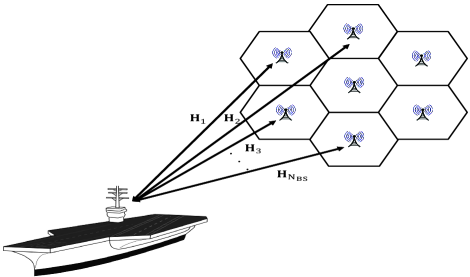
Figure 1: Spectrum-sharing scenario between LTE cellular system and a maritime MIMO radar.

III Radar-LTE Spectrum Sharing Approach

In this section, we describe colocated MIMO radars and then present the maximum likelihood (ML) estimate used as our performance metric for the MIMO radar system.

III-A Colocated MIMO Radar

The MIMO radar we consider in this paper is a colocated MIMO radar with $M_{T}$ transmit antennas and $M_{R}$ receive antennas. Let $\mathbf{x}_{\text{Radar}}(t)$ be the signal transmitted from the MIMO radar, defined as

$$\mathbf{x}_{\text{Radar}}(t)=\begin{bmatrix}x_{1}(t)e^{j\omega_{c}t}&x_{2}(t)e^{j\omega_{c}t}&\cdots&x_{M_{T}}e^{j\omega_{c}t}(t)\end{bmatrix}^{T}$$

where $\omega_{c}$ is the carrier angular frequency, $x_{k}(t)$ is the baseband signal from the $k^{\text{th}}$ transmit element and $t\in[0,T_{o}]$ with $T_{o}$ being the observation time. The radar transmit steering vector is defined as

$$\mathbf{a}_{T}(\theta)\triangleq\begin{bmatrix}e^{-j\omega_{c}\tau_{T_{1}}(\theta)}&e^{-j\omega_{c}\tau_{T_{2}}(\theta)}&\cdots&e^{-j\omega_{c}\tau_{T_{M_{T}}}(\theta)}\end{bmatrix}^{T}$$

the radar receive steering vector is defined as

$$\mathbf{a}_{R}(\theta)\triangleq\begin{bmatrix}e^{-j\omega_{c}\tau_{R_{1}}(\theta)}&e^{-j\omega_{c}\tau_{R_{2}}(\theta)}&\cdots&e^{-j\omega_{c}\tau_{R_{M_{R}}}(\theta)}\end{bmatrix}^{T}$$

and the transmit-receive steering matrix is defined as

$$\mathbf{A}(\theta)\triangleq\mathbf{a}_{R}(\theta)\mathbf{a}_{T}^{T}(\theta).$$

Then, the signal received from a single point target at an angle $\theta$ is given by

$$\mathbf{y}_{\text{Radar}}(t)=\alpha\,e^{-j\omega_{D}t}\,\mathbf{A}(\theta)\,\mathbf{x}_{\text{Radar}}(t-\tau(t))$$

where $\tau(t)=\tau_{r}=\tau_{T_{k}}(t)+\tau_{R_{l}}(t)$ is the sum of propagation delays between the target and the $k^{\text{th}}$ transmit element and between the target and the $l^{\text{th}}$ receive element, respectively; and $\alpha$ represents the complex path loss including the propagation loss and the coefficient of reflection.

III-B Maximum Likelihood

We choose maximum likelihood estimate of the three target parameters which are the target’s angle of arrival, the propagation delay time and the Doppler angular frequency as our performance metric for the MIMO radar system. We are interested in studying the degradation in the estimate of each of these parameters due to null space projection of the radar waveform. The ML for the case of no interference and a single target can be written as in [14],

$$(\hat{\theta},\hat{\tau}_{r},\hat{\omega}_{D})_{\text{ML}}=\operatorname*{arg\,max}_{\theta,\tau_{r},\omega_{D}}\frac{\left|\mathbf{a}_{R}^{H}(\theta)\mathbf{E}(\tau_{r},\omega_{D})\mathbf{a}_{T}^{*}(\theta)\right|^{2}}{M_{R}\mathbf{a}_{T}^{H}(\theta)\mathbf{R}_{\mathbf{x}_{\text{Radar}}}^{T}\mathbf{a}_{T}(\theta)}$$ (1)

where

$$\mathbf{R}_{\mathbf{x}_{\text{Radar}}} =\int_{T_{0}}\mathbf{x}_{\text{Radar}}(t)\,\mathbf{x}_{\text{Radar}}^{H}(t)\,dt$$

$$\mathbf{E}(\tau_{r},\omega_{D}) =\int_{T_{0}}\!\mathbf{y}_{\text{Radar}}(t)\,\mathbf{x}_{\text{Radar}}^{H}(t-\tau_{r})\,e^{j\omega_{D}t}\,dt$$

$\tau_{r}$ is the propagation delay that refers to the two way propagation delay between the target and the reference point and $\omega_{D}$ is the Doppler angular frequency.

For orthogonal signal transmission, equation (1) becomes

$$(\hat{\theta},\hat{\tau}_{r},\hat{\omega}_{D})_{\text{ML}}=\operatorname*{arg\,max}_{\theta,\tau_{r},\omega_{D}}\frac{\left|\mathbf{a}_{R}^{H}(\theta)\mathbf{E}(\tau_{r},\omega_{D})\mathbf{a}_{T}^{*}(\theta)\right|^{2}}{M_{R}M_{T}}\cdot$$ (2)

IV Algorithm

In this section, we present a channel-selection algorithm to select the best interference channel on which radar signals are projected. We also present NSP algorithm that performs the null space computation.

IV-A Channel-Selection Algorithm

Our channel-selection algorithm, shown in Algorithm (1), selects the best interference channel onto which radar signals are projected. Based on our system model, we assume that there exist $N_{\text{BS}}$ interference channels $\mathbf{H}_{i},i=1,2,\ldots,N_{\text{BS}}$ between the MIMO radar and the LTE system. Our goal is to select the best interference channel defined as

$$i_{\text{min}} \triangleq\operatorname*{arg\,min}_{1\leq i\leq N_{\text{BS}}}\Arrowvert\mathbf{x}_{\text{Radar}}-{\mathbf{P}}_{\mathbf{V}_{i}}\mathbf{x}_{\text{Radar}}\Arrowvert$$

$$\mathbf{H}_{\text{Best}} \triangleq\mathbf{H}_{i_{\text{min}}}$$

we also seek to avoid the worst interference channel defined as

$$i_{\text{max}} \triangleq\operatorname*{arg\,max}_{1\leq i\leq N_{\text{BS}}}\Arrowvert\mathbf{x}_{\text{Radar}}-{\mathbf{P}}_{\mathbf{V}_{i}}\mathbf{x}_{\text{Radar}}\Arrowvert$$

$$\mathbf{H}_{\text{Worst}} \triangleq\mathbf{H}_{i_{\text{max}}}$$

where $(\mathbf{x}_{\text{Radar}}-{\mathbf{P}}_{\mathbf{V}_{i}}\mathbf{x}_{\text{Radar}})$ is the difference between the original radar waveform $\mathbf{x}_{\text{Radar}}$ and the radar waveform projected onto the null space of $\mathbf{H}_{i}$ and the Euclidean norm of $(\mathbf{x}_{\text{Radar}}-{\mathbf{P}}_{\mathbf{V}_{i}}\mathbf{x}_{\text{Radar}})$ is defined as

$$\Arrowvert\mathbf{x}_{\text{Radar}}-{\mathbf{P}}_{\mathbf{V}_{i}} \mathbf{x}_{\text{Radar}}\Arrowvert=$$

$$\sqrt{(\mathbf{x}_{\text{Radar}}-{\mathbf{P}}_{\mathbf{V}_{i}}\mathbf{x}_{\text{Radar}})^{H}(\mathbf{x}_{\text{Radar}}-{\mathbf{P}}_{\mathbf{V}_{i}}\mathbf{x}_{\text{Radar}})}.$$

We use the blind null space learning algorithm introduced in [15] to estimate the channel state information (CSI) of the $N_{\text{BS}}$ interference channels at the MIMO radar. The projection matrix $\mathbf{P}_{\mathbf{V}_{i}}$ of each of the $N_{\text{BS}}$ interference channels is then found using Algorithm (2). Once Algorithm (1) receives the projection matrices of the interference channels, it selects the best interference channel $\breve{\mathbf{H}}$ and sends it to Algorithm (2) for NSP of radar signals. Selecting the best interference channel using our channel-selection algorithm (i.e. Algorithm (1)) guarantees minimum degradation in the performance of the radar while maintaining no interference to the LTE BS.

Algorithm 1 Channel-Selection Algorithm

  loop

     for $i=1:N_{\text{BS}}$ do

        Estimate CSI of $\mathbf{H}_{i}$.

        Send $\mathbf{H}_{i}$ to Algorithm (2) for null space computation.

        Receive projection matrix $\mathbf{P}_{\mathbf{V}_{i}}$ from Algorithm (2).

     end for

     Find $i_{\text{min}}=\operatorname*{arg\,min}_{1\leq i\leq N_{\text{BS}}}\Arrowvert\mathbf{x}_{\text{Radar}}-{\mathbf{P}}_{\mathbf{V}_{i}}\mathbf{x}_{\text{Radar}}\Arrowvert$.

     Set $\breve{\mathbf{H}}=\mathbf{H}_{i_{\text{min}}}$ as the best interference channel.

     Set $\mathbf{P}_{\breve{\mathbf{V}}}=\mathbf{P}_{\mathbf{V}_{i_{\text{min}}}}$.

     Send $\mathbf{P}_{\breve{\mathbf{V}}}$ to Algorithm (2) to get NSP radar waveform.

  end loop

IV-B Null-Space Projection (NSP) Algorithm

In this section, we present our proposed null-space projection algorithm. We also explain the projection of radar signals onto null space of the best interference channel selected using Algorithm (1). The CSI of each of the $N_{\text{BS}}$ interference channels is first estimated using a blind null space learning algorithm [15]. Algorithm (2) gets the CSI estimates of the interference channels from Algorithm (1) and finds the null space of each $\mathbf{H}_{i}^{N_{R}^{\text{BS}}\times M_{T}}$. This is performed using the singular value decomposition (SVD) theorem as shown in our NSP algorithm (Algorithm (2)). The SVD for the complex $i^{\text{th}}$ interference channel is given by

$$\mathbf{H}_{i}^{N_{R}^{\text{BS}}\times M_{T}}=\mathbf{U}_{i}\mathbf{\Sigma}_{i}^{N_{R}^{\text{BS}}\times M_{T}}\mathbf{V}_{i}^{H}$$

and $\mathbf{\Sigma}_{i}^{N_{R}^{\text{BS}}\times M_{T}}$ is given by

$${\mathbf{\Sigma}_{i}}^{N_{R}^{\text{BS}}\times M_{T}}=\operatorname{diag}(\sigma_{1},... ,\sigma_{k},...,\sigma_{l})\in\mathbb{R}^{N_{R}^{\text{BS}}\times M_{T}}$$

$$\textrm{s.t.}\;\;\;l =\min\{N_{R}^{\text{BS}},M_{T}\}$$

where $\mathbf{U}_{i}$ is the complex unitary matrix, $\bm{\Sigma}_{i}$ is the matrix of singular values, $\sigma_{1}\textgreater\sigma_{2}\textgreater...\textgreater\sigma_{k}\textgreater\sigma_{k+1}=...=\sigma_{l}=0$ and $\mathbf{V}_{i}^{H}$ is the complex unitary matrix. Once the null space of all interference channels is determined, ${\mathbf{\Sigma}_{i}^{\prime}}^{M_{T}\times M_{T}}$ is then calculated as follows

$${\mathbf{\Sigma}_{i}^{\prime}}^{M_{T}\times M_{T}}=\operatorname{diag}(\sigma_{1}^{\prime},...,\sigma_{M_{T}}^{\prime})\in\mathbb{R}^{M_{T}\times M_{T}}$$

$$\textrm{s.t.}\;\;\;\;\;\sigma_{i}^{\prime}=\left\{\begin{array}[]{ll}0,\;\;i\leq k\\ 1,\;\;i>k.\end{array}\right.$$

Algorithm (2) uses ${\mathbf{\Sigma}_{i}^{\prime}}^{M_{T}\times M_{T}}$ for the formation of the projection matrix ${\mathbf{P}}_{\mathbf{V}_{i}}$ that is given by

$$\mathbf{P}_{{\mathbf{V}_{i}}}={\mathbf{V}_{i}}{\mathbf{\Sigma}_{i}^{\prime}}^{M_{T}\times M_{T}}\mathbf{V}_{i}^{H}$$

where $\mathbf{P}_{{\mathbf{V}_{i}}}$ satisfies the following properties:

• $\mathbf{H}_{i}\mathbf{P}_{{\mathbf{V}_{i}}}=0$.

• ${\mathbf{P}_{{\mathbf{V}_{i}}}}^{2}=\mathbf{P}_{{\mathbf{V}_{i}}}$.

Algorithm (1) receives the projection matrices $\mathbf{P}_{{\mathbf{V}_{i}}}$ and uses them to determine the best interference channel $\breve{\mathbf{H}}$ and its corresponding $\mathbf{P}_{\breve{\mathbf{V}}}$, the one with the minimum $\Arrowvert\mathbf{x}_{\text{Radar}}-{\mathbf{P}}_{\mathbf{V}_{i}}\mathbf{x}_{\text{Radar}}\Arrowvert$, which according to our Algorithm (1) is given by

$$i_{\text{min}} =\operatorname*{arg\,min}_{1\leq i\leq N_{\text{BS}}}\Arrowvert\mathbf{x}_{\text{Radar}}-{\mathbf{P}}_{\mathbf{V}_{i}}\mathbf{x}_{\text{Radar}}\Arrowvert$$

$$\breve{\mathbf{H}} =\mathbf{H}_{i_{\text{min}}}$$

$$\mathbf{P}_{\breve{\mathbf{V}}} =\mathbf{P}_{\mathbf{V}_{i_{\text{min}}}}.$$

Algorithm (1) sends $\mathbf{P}_{\breve{\mathbf{V}}}$ to Algorithm (2) where it is used for the projection of the radar waveform. The radar waveform projected onto the null space of $\breve{\mathbf{H}}$ can be written as

$${\breve{\mathbf{x}}_{\text{Radar}}}=\mathbf{P}_{\breve{\mathbf{V}}}\mathbf{x}_{\text{Radar}}.$$ (3)

The radar projected signal given by (3) can be substituted in equation (1) to get the ML estimates of the target’s angle arrival, propagation delay and Doppler angular frequency for the NSP radar waveform.

Algorithm 2 Null-Space Projection (NSP) Algorithm

  if $\mathbf{H}_{i}$ received from Algorithm (1) then

     Perform SVD on $\mathbf{H}_{i}$ (i.e. $\mathbf{H}_{i}=\mathbf{U}_{i}\bm{\Sigma}_{i}\mathbf{V}_{i}^{H}$).

     Find projection matrix $\mathbf{P}_{{\mathbf{V}_{i}}}={\mathbf{V}_{i}}{\mathbf{\Sigma}_{i}^{\prime}}^{M_{T}\times M_{T}}\mathbf{V}_{i}^{H}$.

     Send projection matrix $\mathbf{P}_{{\mathbf{V}_{i}}}$ to Algorithm (1).

  end if

  if $\mathbf{P}_{\breve{\mathbf{V}}}$ received from Algorithm (1) then

     Get NSP radar signal via ${\breve{\mathbf{x}}_{\text{Radar}}}=\mathbf{P}_{\breve{\mathbf{V}}}\mathbf{x}_{\text{Radar}}$.

  end if

V Performance Analysis of the Radar’s Detectable Parameters

In this section, we provide mathematical analysis to study the effect of the projected radar signals on the estimate of the radar’s target detectable parameters. We compare the radar’s detectable values given by the ML estimate in equation (1) for the case of original radar waveform with the radar’s detectable values for the case of the NSP radar waveform. We are interested in three radar’s detectable parameters that are the target’s angle of arrival, the propagation delay and the Doppler angular frequency.

First we investigate the effect of projecting the radar waveform on the estimated angle of arrival. Assuming that $\tau_{r}$ and $\omega_{D}$ are known to the radar, the estimated angle of arrival $\hat{\theta}$ for the non-projected radar waveform case is given by

$$\hat{\theta}_{\text{ML}}\triangleq\theta_{\text{opt}}=\operatorname*{arg\,max}_{\theta_{\text{opt}}}\frac{\left|\mathbf{a}_{R}^{H}(\theta_{\text{opt}})\mathbf{E}(\tau_{r},\omega_{D})\mathbf{a}_{T}^{*}(\theta_{\text{opt}})\right|^{2}}{M_{R}\mathbf{a}_{T}^{H}(\theta_{\text{opt}})\mathbf{R}_{{\mathbf{x}}_{\text{Radar}}}^{T}\mathbf{a}_{T}(\theta_{\text{opt}})}$$ (4)

whereas in the case of the projected radar waveform the ML estimate for the angle of arrival can be written as

$$\hat{\theta}_{\text{ML}^{\text{NSP}}}\triangleq\theta_{\text{opt}}^{\text{NSP}} =\operatorname*{arg\,max}_{\theta_{\text{opt}}^{\text{NSP}}}\frac{\left|\mathbf{a}_{R}^{H}(\theta_{\text{opt}}^{\text{NSP}})\mathbf{E}^{\text{NSP}}(\tau_{r},\omega_{D})\mathbf{a}_{T}^{*}(\theta_{\text{opt}}^{\text{NSP}})\right|^{2}}{M_{R}\mathbf{a}_{T}^{H}(\theta_{\text{opt}}^{\text{NSP}}){\mathbf{R}_{{\mathbf{x}}_{\text{Radar}}}^{T^{\text{NSP}}}}\mathbf{a}_{T}(\theta_{\text{opt}}^{\text{NSP}})}$$ (5)

$$=\operatorname*{arg\,max}_{\theta_{\text{opt}}^{\text{NSP}}}\frac{\left|\mathbf{a}_{R}^{H}(\theta_{\text{opt}}^{\text{NSP}})\mathbf{P}_{\breve{\mathbf{V}}}\mathbf{E}(\tau_{r},\omega_{D})\mathbf{P}_{\breve{\mathbf{V}}}^{H}\mathbf{a}_{T}^{*}(\theta_{\text{opt}}^{\text{NSP}})\right|^{2}}{M_{R}\mathbf{a}_{T}^{H}(\theta_{\text{opt}}^{\text{NSP}})\mathbf{P}_{\breve{\mathbf{V}}}\mathbf{R}_{{\mathbf{x}}_{\text{Radar}}}^{T}\mathbf{P}_{\breve{\mathbf{V}}}^{H}\mathbf{a}_{T}(\theta_{\text{opt}}^{\text{NSP}})}$$

$$=\operatorname*{arg\,max}_{\theta_{\text{opt}}^{\text{NSP}}}\frac{\left|\mathbf{a}_{R}^{H}(\theta_{\text{eff}}^{\text{NSP}})\mathbf{E}(\tau_{r},\omega_{D})\mathbf{a}_{T}^{*}(\theta_{\text{eff}}^{\text{NSP}})\right|^{2}}{M_{R}\mathbf{a}_{T}^{H}(\theta_{\text{eff}}^{\text{NSP}})\mathbf{R}_{{\mathbf{x}}_{\text{Radar}}}^{T}\mathbf{a}_{T}(\theta_{\text{eff}}^{\text{NSP}})}$$

where $\mathbf{a}_{R}^{H}(\theta_{\text{eff}}^{\text{NSP}})=\mathbf{a}_{R}^{H}(\theta_{\text{opt}}^{\text{NSP}})\mathbf{P}_{\breve{\mathbf{V}}}$, $\mathbf{a}_{T}^{*}(\theta_{\text{eff}}^{\text{NSP}})=\mathbf{P}_{\breve{\mathbf{V}}}^{H}\mathbf{a}_{T}^{*}(\theta_{\text{opt}}^{\text{NSP}})$, $\mathbf{a}_{T}^{H}(\theta_{\text{eff}}^{\text{NSP}})=\mathbf{a}_{T}^{H}(\theta_{\text{opt}}^{\text{NSP}})\mathbf{P}_{\breve{\mathbf{V}}}$ and $\mathbf{a}_{T}(\theta_{\text{eff}}^{\text{NSP}})=\mathbf{P}_{\breve{\mathbf{V}}}^{H}\mathbf{a}_{T}(\theta_{\text{opt}}^{\text{NSP}})$. Also $\mathbf{E}^{\text{NSP}}(\tau_{r},\omega_{D})=\mathbf{P}_{\breve{\mathbf{V}}}\mathbf{E}(\tau_{r},\omega_{D})\mathbf{P}_{\breve{\mathbf{V}}}^{H}$ and $\mathbf{R}_{{\mathbf{x}}_{\text{Radar}}}^{T^{\text{NSP}}}=\mathbf{P}_{\breve{\mathbf{V}}}\mathbf{R}_{{\mathbf{x}}_{\text{Radar}}}^{T}\mathbf{P}_{\breve{\mathbf{V}}}^{H}$. Equation (5) shows that the estimated angle of arrival $\theta_{\text{opt}}^{\text{NSP}}$ in the case of the NSP radar waveform is different from the estimated angle of arrival $\theta_{\text{opt}}$ given by (4) in the case of the original radar waveform. Section VI shows that by choosing $\mathbf{H}_{\text{Best}}$ to project using Algorithm (1) and (2) we can achieve almost similar ML results in estimating the angle of arrival for the original radar waveform and the NSP waveform.

The effect of the projected radar waveform in estimating the propagation delay $\tau_{r}$ is also investigated. Assuming that $\theta$ and $\omega_{D}$ are known to the radar, the estimated propagation delay $\hat{\tau}_{r}$ for the non-projected radar waveform case is given by

$$(\hat{\tau}_{r})_{\text{ML}}\triangleq{\tau_{r,\text{opt}}}=\operatorname*{arg\,max}_{{\tau_{r,\text{opt}}}}\frac{\left|\mathbf{a}_{R}^{H}(\theta)\mathbf{E}({\tau_{r,\text{opt}}},\omega_{D})\mathbf{a}_{T}^{*}(\theta)\right|^{2}}{M_{R}\mathbf{a}_{T}^{H}(\theta)\mathbf{R}_{{\mathbf{x}}_{\text{Radar}}}^{T}\mathbf{a}_{T}(\theta)}$$ (6)

where $\mathbf{E}(\tau_{r,\text{opt}},\omega_{D})=\int_{T_{0}}\!\mathbf{y}_{\text{Radar}}(t)\,\mathbf{x}_{\text{Radar}}^{H}(t-\tau_{r,\text{opt}})\,e^{j\omega_{D}t}\,dt$ is equivalent to $\int_{T_{0}}\!\alpha\,e^{-j\omega_{D}t}\,\mathbf{A}(\theta)\,\mathbf{x}_{\text{Radar}}(t-\tau)\,\mathbf{x}_{\text{Radar}}^{H}(t-\tau_{r,\text{opt}})\,e^{j\omega_{D}t}\,dt$. Since the radar waveforms are orthogonal waveforms, the objective function in equation (6) can be maximized when $\mathbf{E}(\tau_{r,\text{opt}},\omega_{D})$ is maximized and can be achieved when $\tau_{r,\text{opt}}=\tau$. In the case of the projected radar waveform the ML estimate for the propagation delay can be written as

$$(\hat{\tau}_{r})_{\text{ML}^{\text{NSP}}}\triangleq{\tau_{r,\text{opt}}^{\text{NSP}}}=\operatorname*{arg\,max}_{\tau_{r,\text{opt}}^{\text{NSP}}}\frac{\left|\mathbf{a}_{R}^{H}(\theta)\mathbf{P}_{\breve{\mathbf{V}}}\mathbf{E}({\tau_{r,\text{opt}}^{\text{NSP}}},\omega_{D})\mathbf{P}_{\breve{\mathbf{V}}}^{H}\mathbf{a}_{T}^{*}(\theta)\right|^{2}}{M_{R}\mathbf{a}_{T}^{H}(\theta)\mathbf{P}_{\breve{\mathbf{V}}}\mathbf{R}_{{\mathbf{x}}_{\text{Radar}}}^{T}\mathbf{P}_{\breve{\mathbf{V}}}^{H}\mathbf{a}_{T}(\theta)}\cdot$$ (7)

Again the objective function in (7) can be maximized when $\mathbf{E}(\tau_{r,\text{opt}}^{\text{NSP}},\omega_{D})$ is maximized and can be achieved when $\tau_{r,\text{opt}}^{\text{NSP}}=\tau$. Therefore, projecting the radar waveforms has no effect on the estimated propagation delay and equation (7) gives an estimate for the propagation delay similar to the one given by equation (6).

Furthermore, the effect of the projected radar waveform in estimating the Doppler angular frequency $\omega_{D}$ is also investigated. Assuming that $\theta$ and $\tau_{r}$ are known to the radar, the Doppler angular frequency $\hat{\omega}_{D}$ for the non-projected radar waveform case is given as

$$(\hat{\omega}_{D})_{\text{ML}}\triangleq{\omega_{D,\text{opt}}}=\operatorname*{arg\,max}_{{\omega_{D,\text{opt}}}}\frac{\left|\mathbf{a}_{R}^{H}(\theta)\mathbf{E}({\tau_{r}},\omega_{D,\text{opt}})\mathbf{a}_{T}^{*}(\theta)\right|^{2}}{M_{R}\mathbf{a}_{T}^{H}(\theta)\mathbf{R}_{{\mathbf{x}}_{\text{Radar}}}^{T}\mathbf{a}_{T}(\theta)}$$ (8)

where $\mathbf{E}(\tau_{r},\omega_{D,\text{opt}})=\int_{T_{0}}\!\mathbf{y}_{\text{Radar}}(t)\,\mathbf{x}_{\text{Radar}}^{H}(t-\tau_{r})\,e^{j\omega_{D,\text{opt}}t}\,dt$ is equivalent to $\int_{T_{0}}\!\alpha\,e^{-j\omega_{D}t}\,\mathbf{A}(\theta)\,\mathbf{x}_{\text{Radar}}(t-\tau)\,\mathbf{x}_{\text{Radar}}^{H}(t-\tau_{r})\,e^{j\omega_{D,\text{opt}}t}\,dt$ and $\tau=\tau_{r}$ in this case. Since the radar waveforms are orthogonal waveforms, the objective function in equation (6) can be maximized when $\mathbf{E}(\tau_{r},\omega_{D,\text{opt}})$ is maximized and can be achieved when $\omega_{D,\text{opt}}=\omega_{D}$. In the case of the projected radar waveform the ML estimate for the propagation delay can be written as

$$(\hat{\omega}_{D})_{\text{ML}^{\text{NSP}}}\triangleq{\omega_{D,\text{opt}}^{\text{NSP}}}=\operatorname*{arg\,max}_{\omega_{D,\text{opt}}^{\text{NSP}}}\frac{\left|\mathbf{a}_{R}^{H}(\theta)\mathbf{P}_{\breve{\mathbf{V}}}\mathbf{E}({\tau_{r}},\omega_{D,\text{opt}}^{\text{NSP}})\mathbf{P}_{\breve{\mathbf{V}}}^{H}\mathbf{a}_{T}^{*}(\theta)\right|^{2}}{M_{R}\mathbf{a}_{T}^{H}(\theta)\mathbf{P}_{\breve{\mathbf{V}}}\mathbf{R}_{{\mathbf{x}}_{\text{Radar}}}^{T}\mathbf{P}_{\breve{\mathbf{V}}}^{H}\mathbf{a}_{T}(\theta)}\cdot$$ (9)

The objective function in (9) can be maximized when $\mathbf{E}(\tau_{r,\text{opt}}^{\text{NSP}},\omega_{D})$ is maximized and can be achieved when $\omega_{D,\text{opt}}^{\text{NSP}}=\omega_{D}$. Therefore, projecting the radar waveforms has no effect on the estimated Doppler angular frequency and equation (9) gives an estimate for the propagation delay that is similar to the one given by equation (8).

VI Simulations

In this section, we simulate the presented MIMO radar and LTE spectrum sharing scenario and study its impact on the performance of the radar in estimating the detectable target parameters. The simulation parameters used are listed in Table I. Algorithm (1) and Algorithm (2) were applied in MATLAB to select the best interference channel $\mathbf{H}_{\text{Best}}$ and project the radar signal onto it. By applying Algorithm (1) and Algorithm (2), we are able to minimize the degradation in the radar performance as projecting the radar waveform onto $\mathbf{H}_{\text{Best}}$ results in a NSP waveform that is closer to the original radar waveform than the NSP waveform in the case of projecting the radar waveform onto $\mathbf{H}_{\text{Worst}}$. We compared the radar estimated detectable target parameters, using ML estimate, in the case of the original radar waveform and the two cases of NSP radar waveform, first when choosing $\mathbf{H}_{\text{Best}}$ to project and second when choosing $\mathbf{H}_{\text{Worst}}$ to project.

TABLE I: MIMO Radar System Parameters

Parameters	Notations	Values
Radar/LTE shared RF band	-	$3550-3650$ MHz
Radar waveform bandwidth	$B$	10 MHz
Radar transmit antennas	$M_{T}$	10
Radar receive antennas	$M_{R}$	7
Carrier frequency	$f_{c}$	3.55 GHz
Wavelength	$\lambda$	8.5 cm
Inter-element antenna spacing	$3\lambda/4$	6.42 cm
Radial velocity	$v_{r}$	2000 m/s
Speed of light	$c$	3 $\times$ $10^{8}$ m/s
Observation time	$T_{0}$	1 ms
Target distance from the radar	$r_{0}$	5000 m
Target angle	$\theta$	$0^{\circ}$
Doppler frequency shift	$f_{d}$	$2v_{r}/\lambda$
Doppler angular frequency	$\omega_{D}$	$2\omega_{c}v_{r}/c=2\pi f_{d}$
propagation delay	$\tau_{r}$	$2r_{0}/c$
Path loss	$\alpha$	$\alpha_{ji}e^{-j\omega_{c}\tau_{r}}$

In Figure 2, we compare the estimated angles when using the ML estimate described in equation (1) for the original radar waveform with the estimated angles using the ML estimate for both of the NSP radar waveform onto $\mathbf{H}_{\text{Best}}$ and the NSP radar waveform onto $\mathbf{H}_{\text{Worst}}$. Figure 2 shows that choosing $\mathbf{H}_{\text{Best}}$ to project can cause less degradation in estimating the angle of arrival than choosing $\mathbf{H}_{\text{Worst}}$ to project.

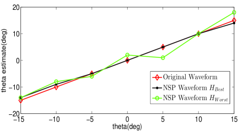
Figure 2: Target direction $\hat{\theta}$ estimation using ML estimate in the case of the original radar waveform, the NSP radar waveform projected onto $\mathbf{H}_{\text{Best}}$ and the NSP radar waveform projected onto $\mathbf{H}_{\text{Worst}}$.

In Figure 3, we compare the estimated propagation delay $\hat{\tau}_{r}$ when using the ML estimate for the original radar waveform with the estimated propagation delay using the ML estimate for both of the NSP radar waveform onto $\mathbf{H}_{\text{Best}}$ and the NSP radar waveform onto $\mathbf{H}_{\text{Worst}}$. Figure 3 shows that projecting the radar waveform does not affect the estimated propagation delay and results in an estimated value that is similar to the one obtained when using the original radar waveform. Similarly, Figure 4 shows that the estimated Doppler frequency shift $\hat{f}_{d}$ when using the projected radar waveform, i.e. for the case of NSP radar waveform onto $\mathbf{H}_{\text{Best}}$ and the case of NSP radar waveform onto $\mathbf{H}_{\text{Worst}}$ is similar to the estimated $\hat{f}_{d}$ when using the original radar waveform.

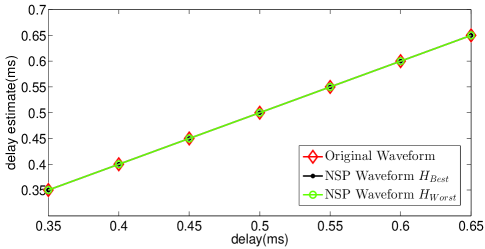
Figure 3: Propagation delay $\hat{\tau}_{r}$ estimation using ML estimate in the case of the original radar waveform, the NSP radar waveform projected onto $\mathbf{H}_{\text{Best}}$ and the NSP radar waveform projected onto $\mathbf{H}_{\text{Worst}}$.

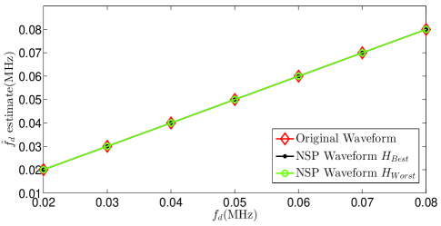
Figure 4: Doppler frequency shift $\hat{f}_{d}$ estimation using ML estimate in the case of the original radar waveform, the NSP radar waveform projected onto $\mathbf{H}_{\text{Best}}$ and the NSP radar waveform projected onto $\mathbf{H}_{\text{Worst}}$.

VII Conclusion

In this paper, we presented a spectrum sharing scenario between a MIMO radar and LTE cellular system with multiple BSs. We proposed a channel-selection algorithm and NSP algorithm to select the best interference channel and project the radar signal onto it. Our proposed algorithms guarantee a minimum degradation in the radar’s performance by selecting the best interference channel for the NSP of the radar signal. We showed through mathematical analysis the effect of projecting the radar signal on the radar’s target detectable parameters. Our analysis showed that when using the ML estimate, the estimated propagation delay and the estimated Doppler angular frequency in the case of the original radar waveform are similar to the estimated values in the case of the projected radar waveform whereas the estimated angle of arrival is affected when projecting the radar waveform. We showed through our simulation results that the estimated propagation delay and Doppler frequency shift are not affected when using the NSP radar waveforms and that the loss in the radar performance in detecting the angle of arrival is minimal when our proposed spectrum sharing algorithm is used to select the best channel onto which radar signals are projected.

References

- [1] E. Axell, G. Leus, E. Larsson, and H. Poor, “Spectrum sensing for cognitive radio : State-of-the-art and recent advances,” Signal Processing Magazine, IEEE, vol. 29, no. 3, pp. 101–116, 2012.
- [2] National Telecommunications and Information Administration (NTIA), “An assessment of the near-term viability of accommodating wireless broadband systems in the 1675-1710 MHz, 1755-1780 MHz, 3500-3650 MHz, 4200-4220 MHz, and 4380-4400 MHz bands (Fast Track Report).” Online, October 2010.
- [3] Federal Communications Commission (FCC), “In the matter of revision of parts 2 and 15 of the commission’s rules to permit unlicensed national information infrastructure (U-NII) devices in the 5 GHz band.” MO&O, ET Docket No. 03-122, June 2006.
- [4] Federal Communications Commission (FCC), “FCC proposes innovative small cell use in 3.5 GHz band.” Online: http://www.fcc.gov/document/fcc-proposes-innovative-small-cell-use-35-ghz-band, December 12, 2012.
- [5] A. Khawar, A. Abdel-Hadi, and T. Clancy, “Spectrum sharing between s-band radar and lte cellular system: A spatial approach,” in Dynamic Spectrum Access Networks (DYSPAN), 2014 IEEE International Symposium on, pp. 7–14, April 2014.
- [6] S. Sodagari, A. Khawar, T. C. Clancy, and R. McGwier, “A projection based approach for radar and telecommunication systems coexistence,” in IEEE Global Communications Conference (GLOBECOM), 2012.
- [7] J. Li and P. Stoica, “Mimo radar with colocated antennas,” Signal Processing Magazine, IEEE, vol. 24, no. 5, pp. 106–114, 2007.
- [8] A. Khawar, A. Abdel-Hadi, T. Clancy, and R. McGwier, “Beampattern analysis for mimo radar and telecommunication system coexistence,” in Computing, Networking and Communications (ICNC), 2014 International Conference on, pp. 534–539, Feb 2014.
- [9] H. Deng and B. Himed, “Interference mitigation processing for spectrum-sharing between radar and wireless communications systems,” Aerospace and Electronic Systems, IEEE Transactions on, vol. 49, pp. 1911–1919, July 2013.
- [10] H. Shajaiah, A. Khawar, A. Abdel-Hadi, and T. Clancy, “Resource allocation with carrier aggregation in lte advanced cellular system sharing spectrum with s-band radar,” in Dynamic Spectrum Access Networks (DYSPAN), 2014 IEEE International Symposium on, pp. 34–37, April 2014.
- [11] H. Shajaiah, A. Abdel-Hadi, and C. Clancy, “Spectrum sharing between public safety and commercial users in 4g-lte,” in Computing, Networking and Communications (ICNC), 2014 International Conference on, pp. 674–679, Feb 2014.
- [12] H. Shajaiah, A. Abdel-Hadi, and C. Clancy, “Multi-Application Resource Allocation with Users Discrimination in Cellular Networks,” in Accepted in PIMRC, 2014.
- [13] H. Shajaiah, A. Abdel-Hadi, and C. Clancy, “Utility proportional fairness resource allocation with carrier aggregation in 4g-lte,” in Military Communications Conference, MILCOM 2013 - 2013 IEEE, pp. 412–417, Nov 2013.
- [14] J. Li and P. Stoica, MIMO Radar Signal Processing. Wiley-IEEE Press, 2008.
- [15] Y. Noam and A. Goldsmith, “Blind null-space learning for mimo underlay cognitive radio with primary user interference adaptation,” Wireless Communications, IEEE Transactions on, vol. 12, no. 4, pp. 1722–1734, 2013.