Robustness of Quantum Spin Hall Effect in an External Magnetic Field

Abstract

The edge states in the quantum spin Hall effect are expected to be protected by time reversal symmetry. The experimental observation of the quantized conductance was reported in the InAs/GaSb quantum well [Du et al, arXiv:1306.1925], up to a large magnetic field, which raises a question on the robustness of the edge states in the quantum spin Hall effect under time reversal symmetry breaking. Here we present a theoretical calculation on topological invariants for the Benevig-Hughes-Zhang model in an external magnetic field, and find that the quantum spin Hall effect retains robust up to a large magnetic field. The critical value of the magnetic field breaking the quantum spin Hall effect is dominantly determined by the band gap at the $\Gamma$ point instead of the indirect band gap between the conduction and valence bands. This illustrates that the quantum spin Hall effect could persist even under time reversal symmetry breaking.

I Introduction

The quantum spin Hall effect (QSHE) is a novel state of quantum matter, in which an electric field can generate a transverse spin current Moore-10nature ; Hazan-10rmp ; Qi-11rmp ; Shen-book . A quantum spin Hall system has a bulk gap between the conduction and valence bands meanwhile processing a pair of gapless helical edge states surrounding the boundariesKane-05prla ; Bernevig-06science ; Liu-08prl . The gapless helical edge states give rise to a quantized conductance in a two-terminal measurement, which has been observed experimentally in HgTe/CdTe quantum well Konig-07science and in InAs/GaSb quantum well Knez-11prl . While these edge states are expected to be protected by time reversal symmetry Kane-05prlb , a recent measurement of QSHE in the InAs/GaSb quantum well surprisingly indicates that the quantized plateau of conductance persists up to a 12 T (Tesla) in-plane magnetic field, or an 8 T perpendicular magnetic fieldDu-13xxx ; Du2014 . This observation raises a question on the robustness of QSHE under time reversal symmetry breaking.

The electronic backscattering in the gapless edge states is prohibited by time reversal symmetry, so that the transport is robust against disorders respecting the symmetryXu-06prb ; Wu-06prl ; Onoda-07prl . An external magnetic field breaks time reversal symmetry and leads to two important effects: a Peierls phase to the orbital motion, and a Zeeman split to the spin motion. The interplay between the spin-orbit coupling and the Zeeman coupling may break QSHE, where the edge states open a small sub-gap Konig-08JPSJ ; Yang-11prl , and the robust transports for QSHE break down similar to the result caused by the finite size effectZhou-08prl .

In this paper, we present theoretical calculations on topological invariants of the Bernevig-Hughes-Zhang (BHZ) model for the QSHE, under an external magnetic field. Our main work focuses on the orbital motion (i.e., the Landau level forming) effects of magnetic field, ignoring the Zeeman couplings. This is reasonable for QSHE materials with small $g$ factors. Furthermore, due to the absence of spin-flip (e.g., Rashba like spin-orbital coupling) terms, the physical spin $S_{z}$ is preserved and the system can be decoupled into two components with opposite $S_{z}$. This makes the two spin-dependent Chern numbers (for spin up and down components respectively) well defined, even in the presence of an external field. Correspondingly, it is found that the edge states persist up to a large magnetic field, until some band crossing happens. The band gap at the $\Gamma$ point instead of the indirect gap plays an important role in determining the critical magnetic field to break down the QSHE. However, when the symmetry preserving $S_{z}$ is also broken by spin-flip terms coupling two spin components, usually the edge states are no longer robust. At the end the effect of a finite Zeeman coupling for perpendicular field is studied, and the critical values the Zeeman field are presented. The effects of other spin-orbital coupling and the in-plane Zeeman field are also discussed.

II Model and solutions

We start with the BHZ model defined, in the basis $\{\left|s\uparrow\right\rangle,\left|p\uparrow\right\rangle,\left|s\downarrow\right\rangle,\left|p\downarrow\right\rangle\}$, for the QSHE in quantum wells Bernevig-06science ,

$$H_{0}(\mathbf{k})=\left(\begin{matrix}h_{+}(\mathbf{k})&0\\ 0&h_{-}(\mathbf{k})\end{matrix}\right)$$ (1)

where $h_{\pm}(\mathbf{k})=\epsilon(\mathbf{k})\sigma_{0}+\bm{d}_{\pm}\cdot\bm{\sigma}$ with denoting $\mathbf{d}_{\pm}=[\pm Ak_{x},-Ak_{y},\mathcal{M}(\mathbf{k})]$, $\epsilon(\mathbf{k)}=-Dk^{2}$, $\mathcal{M}(\mathbf{k})=\Delta-Bk^{2}$, $k^{2}=k_{x}^{2}+k_{y}^{2}$, $k_{\pm}=k_{x}\pm ik_{y}$, and $\mathbf{\sigma}_{i}$ are the Pauli matrices for the orbital $\{\left|s\right\rangle,\left|p\right\rangle\}$. The system possesses time reversal symmetry implied by the relation between two spin components, $h_{-}(\mathbf{k})=h_{+}^{*}(-\mathbf{k})$. This model has been used to describe the QSHE in HgTe/CdTe and InAs/GaSb quantum wells Bernevig-06science ; Liu-08prl .

The Hamiltonian (1) can be exactly diagonalized, and two branches of doubly degenerated eigenenergies are:

$$E_{s}^{\pm}(\mathbf{k})=\epsilon(\mathbf{k})+s|\mathbf{d}_{\pm}|=\epsilon(\mathbf{k})+s\sqrt{M^{2}(\mathbf{k})+A^{2}k^{2}},$$ (2)

where $s=+1$ ($-1$) stands for the conduction (valence) band, and the superscript $\pm$ of $E_{s}^{\pm}(\bm{k})$ stands for spin up (down) component,which are degenerated here. The term $\epsilon(\bm{k})$ breaks the particle-hole symmetry. When $|D|^{2}<|B|^{2}$, there is an energy gap between the conduction band $E_{s=+1}^{\pm}(\bm{k})$ and the valence band $E_{s=-1}^{\pm}(\bm{k})$. The gap at $\Gamma$ ($\bm{k}=0$) is determined by $2\Delta$. According to the $Z_{2}$ classification, the system can be classified as a topologically trivial insulator ($B\cdot\Delta<0$) or nontrivial ($B\cdot\Delta>0$) insulatorLu-10prb when the Fermi level is located within the gap. For a large value of $\left|\Delta\right|$, the band gap (the minimum band separation in the Brillouin zone, which may not be located at $\Gamma$) is approximately given by $2|A|\sqrt{\Delta/B}$ when $B\cdot\Delta>0$ as shown in Fig. 1.

Due to the decoupling between the two spin components $h_{\pm}$, the physical spin operator $\mathbf{S}_{z}=\tau_{z}\otimes\sigma_{0}$ commutes with $H_{0}$, and has good quantum numbers $S_{z}=\pm 1$, where $\tau_{i}$ refer to Pauli matrices for physical spin and $\sigma_{0}$ is a $2\times 2$ identity matrix. This symmetry guarantees that for each spin component ($h_{+}$ or $h_{-}$), a spin-dependent Chern number is well defined. The Chern numbers for these two spin components ($\pm$) are

$$n_{\pm}=\pm\frac{1}{2}[\mathrm{sgn}(B)+\mathrm{sgn}(\Delta)],$$ (3)

when the Fermi energy lies in the bulk gapLu-10prb . As a consequence, the Hall conductance for the whole system is always zero, $\sigma_{xy}=\left(n_{+}+n_{-}\right)\frac{e^{2}}{h}=0$ due to time reversal symmetry, as expected. On the other hand, the spin Chern number Sheng-06prl defined as $n_{s}=\left(n_{+}-n_{-}\right)/2$ equals $1$ or $-1$ when $B\cdot\Delta>0$ , which indicates the spin Hall conductance is $\sigma_{s}=n_{s}\frac{e}{4\pi}$, and the system exhibits the QSHE.

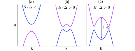
Figure 1: Schematic of two-dimensional energy spectra of the quantum well systems. (a) the normal state of $B\cdot\Delta<0$. (b) the band inverted state of $B\cdot\Delta>0$. (c) the band inverted state of $B\cdot\Delta>0$ with a large gap at $k=0$ but a small bulk gap such as in the InAs/GaSb quantum well.

Parameters	$\Delta$ [eV]	B [eV$\mathrm{nm}^{2}$]	D [eV$\mathrm{nm}^{2}$]	A [eV$\mathrm{nm}$]
HgTe	-0.010	-0.686	-0.512	0.365
InAs/GaSb	-0.008	-0.400	-0.300	0.023

Table 1: The Bernevig-Hughes-Zhang model parameters for quantum wells in the band inverted regime. Parameters for HgTe/CdTe quantum well are at $d=7$ nm Konig-08JPSJ . For the InAs/GaSb quantum well, $\Delta$ is deduced from the experiment, and other parameters are taken to have a ratio of the $2\Delta$ to to the indirect gap about 4 Knez-11prl .

A perpendicular magnetic field $\mathbf{B}=\mathcal{B}\mathbf{\hat{z}}$ (we assume $\mathcal{B}>0$ without losing generality) breaks the time reversal symmetry, but $\mathbf{S}_{z}$ is still preserved, which makes it possible to calculate the Chern numbers for each spin component $h_{\pm}$, separately. In the absence of the Zeeman splitting, the magnetic field only manifests itself on the orbital motion. Similar to the case of two-dimensional electron gas in a perpendicular magnetic fieldShen-04prl , the wave vector in Eq. (1) is replaced by the substitution, $\mathbf{k}\rightarrow-i\nabla_{\mathbf{r}}+e\mathbf{A}/\hbar$, where $\mathbf{A}$ is the vector potential so that $\mathbf{B}=\nabla\times\mathbf{A}$. Choosing the Landau gauge $\mathbf{A}=(-\mathcal{B}y,0,0)$, which preserves the translational symmetry in $x$ direction, we can take the eigen wavefunction as the form $\varphi(x,y)=e^{ikx}\phi(y)$. We define the ladder operators in the following form,

$$a^{\dagger}(k)=\dfrac{1}{\sqrt{2}}(\dfrac{y-y_{0}}{\ell_{B}}-\ell_{B}\partial_{y}),$$ (4)

$$a(k)=\dfrac{1}{\sqrt{2}}(\dfrac{y-y_{0}}{\ell_{B}}+\ell_{B}\partial_{y}),$$ (5)

where $y_{0}=\ell_{B}^{2}k$ is the guiding center of the wave package, and $\ell_{B}=\sqrt{\hbar/e\mathcal{B}}$ is the magnetic length. These two operators obey the canonical commutation relation, $[a(k),a^{{\dagger}}(k^{\prime})]=1$. Thus, the Hamiltonian can be re-expressed in terms of the ladder operators as

$$\begin{array}[]{cc}h_{\pm}(a,a^{\dagger})&=\omega_{2}(a^{\dagger}a+\dfrac{1}{2})\sigma_{0}\pm\eta(a^{\dagger}\sigma_{+}+a\sigma_{-})\\ &+\left[\Delta+\omega_{1}(a^{\dagger}a+\dfrac{1}{2})\right]\sigma_{z}\end{array}$$ (6)

with $\eta=-\sqrt{2}A/\ell_{B}\dfrac{}{}$, $\omega_{1}=-2B/\ell_{B}^{2}$ and $\omega_{2}=-2D/\ell_{B}^{2}$. It is now easy to analytically solve the eigen-problems for $h_{\pm}$, respectively.

For the spin-up component $h_{+}$, the eigenenergies are

$$E_{n,k,s}^{+}= \dfrac{1}{2}[\omega_{1}+2n\omega_{2}+s\sqrt{(\omega_{2}+2(\Delta+n\omega_{1}))^{2}+4n\eta^{2}}],$$ (7)

where $\eta$ and $\omega_{1,2}$ are the functions of $\mathcal{B}$. The corresponding eigenstates $\left|n,k,s\right\rangle_{+}$ have a degeneracy $N_{\phi}=\Omega/(2\pi\ell_{B}^{2})$ with $\Omega$ the area of the two-dimensional system for different wave vectors $k$. Explicitly, the two-component eigen-function for $h_{+}$ is given by

$$\left|n,k,s\right\rangle_{+}=\left(\begin{array}[]{c}\cos\theta_{ns}\phi_{n,k}\\ \sin\theta_{ns}\phi_{n-1,k}\end{array}\right)$$ (8)

Where $\phi_{n,k}(y)=\frac{1}{\sqrt{n!2^{n}\ell_{B}\sqrt{\pi}}}e^{ikx-(y-y_{0})^{2}/2\ell_{B}^{2}}\mathcal{H}_{n}(\frac{y-y_{0}}{\ell_{B}})$ is the eigenstate of the number operator $a^{{\dagger}}a$ with an integer eigenvalue $n$, and $\mathcal{H}_{n}$ are the Hermite polynomials defined as $\mathcal{H}_{n}({\xi})=(-1)^{n}e^{\xi^{2}}\frac{\partial^{n}}{\partial\xi^{n}}e^{-\xi^{2}}$. Notice there are two Landau levels with $s=\pm$ for $n\geqslant 1$, but only $s=\mathrm{sgn}\left(\omega_{2}+2\Delta\right)$ for $n=0$. For $n=0$, $\theta_{n=0,s}=0$. Otherwise, for $n\geqslant 1$, $\tan\theta_{n,s}=s\sqrt{1+u_{n}^{2}}-u_{n}$ with $u_{n}=\left[\omega_{2}+2(\Delta+n\omega_{1})\right]/\sqrt{4n\eta^{2}}$.

For the spin-down component $h_{-}$, the eigenenergies are

$$E_{n,k,s}^{-}= \dfrac{1}{2}[2n\omega_{2}-\omega_{1}+s\sqrt{(\omega_{2}-2(\Delta+n\omega_{1}))^{2}+4n\eta^{2}}],$$ (9)

and the corresponding two-component eigen-function for $h_{-}$ is given by

$$\left|n,k,s\right\rangle_{-}=\left(\begin{array}[]{c}-\sin\theta_{n,s}^{-}\phi_{n-1,k}\\ \cos\theta_{n,s}^{-}\phi_{n,k}\end{array}\right)$$ (10)

Similarly, there are two Landau levels with $s=\pm$ for $n\geqslant 1$, but only $s=\mathrm{sgn}\left(\omega_{2}-2\Delta\right)$ for $n=0$. For $n=0$, $\theta_{n=0,s}^{-}=0$. Otherwise, for $n\geqslant 1$, $\tan\theta_{n,s}^{-}=s\sqrt{1+v_{n}^{2}}-v_{n}$ with $v_{n}=\left[\omega_{2}-2(\Delta+n\omega_{1})\right]/\sqrt{4n\eta^{2}}$.

When the Fermi energy lies in the bulk gap, as in the following calculations, the Landau levels [Eq. (7)] are divided into two sets: the electron-like Landau levels $E_{n,k,s=+}^{m}$ evolving from the conduction band, and the hole-like Landau levels $E_{n,k,s=-}^{m}$ evolving from the valence band for $n>0$, with the superscript $m=\pm$ referring to spin components $h_{\pm}$. The $0$th Landau level of $h_{+}$ is electron-like (hole-like) if $2\Delta+\omega_{2}>0$ ($<0$), so we can denote it as $E_{0,k,+}^{+}=\frac{\omega_{1}}{2}+\frac{\omega_{2}}{2}+\Delta$ ($E_{0,k,-}^{+}=\frac{\omega_{1}}{2}+\frac{\omega_{2}}{2}+\Delta$). Analogously, for the $h_{-}$, the $0$th Landau level is electron-like (hole-like) if $2\Delta-\omega_{2}<0$ ($>0$), and we denote $E_{0,k,+}^{-}=-\frac{\omega_{1}}{2}+\frac{\omega_{2}}{2}-\Delta$ ($E_{0,k,-}^{-}=-\frac{\omega_{1}}{2}+\frac{\omega_{2}}{2}-\Delta$). There is always a finite gap between the electron-like Landau levels and the hole-like Landau levels. In other words, the gap between the conduction and valence bands never close in a finite magnetic field when the Zeeman splitting is ignored.

The developments of the Landau levels $E_{n,k,s}^{+}(\mathcal{B})$ and $E_{n,k,s}^{-}(\mathcal{B})$ under the magnetic field for some typical parameters associated with realistic quantum wells are plotted in Fig. 2. One important observation in Figs. 2(a), (b), (d) and (e) is that, for one spin component, the Landau levels from the conduction band (electron-like) $E_{n,k,s}^{\pm}(\mathcal{B})$ never cross with those from the valance band (hole-like) $E_{n,k,-s}^{\pm}(\mathcal{B})$. In other words, the orbital motion of electrons in a magnetic field cannot lead to the gap closing between the conduction and valence bands. This is one of the main results in this work. As a result, with the increasing of magnetic field $\mathcal{B}$, possible topological transitions (band crossings) in the bulk gap can happen only when both spin components are considered together, as shown in Fig. 2(c) and (f). The calculation of the spin Chern numbers is presented in the following section.

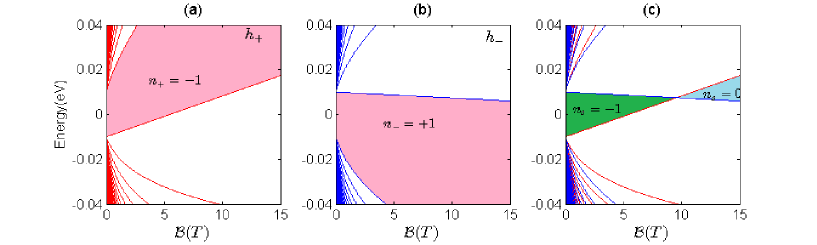
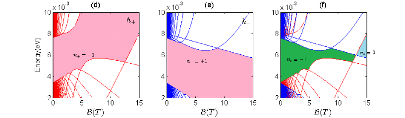
Figure 2: The Landau levels as functions of a perpendicular magnetic field $\mathcal{B}$ in a unit of tesla (T). The upper row is for the HgTe quantum well and the lower row is for the InAs/GaSb quantum well. The left, middle and right columns correspond to $h_{+}$ (spin up), $h_{-}$ (spin down) and $H_{0}$ (whole system), respectively. The shaded region is the bulk gap between the conduction and valence band, with topological invariants labelled. Model parameters are listed in Table.1.

III Chern numbers in a magnetic field

The main result in this section is summarized as follows: in the presence of a perpendicular magnetic field, when the Fermi level lies in the bulk gap of $h_{+}$ and $h_{-}$, the spin-dependent Hall conductivities are always

$$\sigma_{xy}^{\pm}\equiv n_{\pm}\frac{e^{2}}{h}=\pm\frac{1}{2}\left[\mathrm{sgn}(B)+\mathrm{sgn}(\Delta)\right]\frac{e^{2}}{h}.$$ (11)

It means that for any finite field $\mathcal{B}$, $\sigma_{\pm}=0$ if $B\cdot\Delta<0$ while $\sigma_{\pm}=\mp e^{2}/h$ if $B\cdot\Delta>0$ when the Fermi level is located within the band gap between the conduction and valence bands. These results, which can be calculated explicitly from the Kubo formula, or the formula for Chern number Lu-10prb , are identical to those in the absence of magnetic field, i.e., $\mathcal{B}=0$.

III.1 A general expression

In the following, we present the detailed calculations of these Hall conductivities at zero temperature. By using the Kubo formula, the Chern numbers for spin component $m=\pm$ are given by

$$n_{m}= -\dfrac{2\pi\hbar^{2}}{\Omega}\sum_{k}\sum_{n\neq n^{\prime},s,s^{\prime}}\left[f(E_{n,k,s}^{m}-\mu)-f(E_{n^{\prime},k^{\prime},s^{\prime}}^{m}-\mu)\right]$$ (12)

$$\dfrac{\mathrm{Im}\left[{}_{m}\left\langle n,k,s\right|\hat{v}_{x}^{m}\left|n^{\prime},k,s^{\prime}\right\rangle_{mm}\left\langle n^{\prime},k,s^{\prime}\right|\hat{v}_{y}^{m}\left|n,k,s\right\rangle_{m}\right]}{(E_{n,k,s}^{m}-E_{n^{\prime},k,s^{\prime}}^{m})^{2}},$$

where $f(x)$ is the Fermi-Dirac distribution function, $\mu$ is the Fermi energy and the velocity operators can be obtained by evaluating $\hat{v}_{x}^{\pm}=\partial h_{\pm}/\hbar\partial k_{x}$ and $\hat{v}_{y}^{\pm}=\partial h_{\pm}/\hbar\partial k_{y}$ with the substitution $\mathbf{k}\rightarrow-i\nabla_{\mathbf{r}}+e\mathbf{A}/\hbar$,

$$\hat{v}_{x}^{\pm}=-\dfrac{\ell_{B}}{\sqrt{2}\hbar}\left(\begin{matrix}\omega_{+}(a^{{\dagger}}+a)&\pm\eta\\ \pm\eta&\omega_{-}(a^{{\dagger}}+a)\end{matrix}\right),$$ (13)

$$\hat{v}_{y}^{\pm}=\dfrac{i\ell_{B}}{\sqrt{2}\hbar}\left(\begin{matrix}\omega_{+}(a^{{\dagger}}-a)&-\eta\\ +\eta&\omega_{-}(a^{{\dagger}}-a)\end{matrix}\right),$$ (14)

where $\omega_{\pm}=\pm\omega_{1}+\omega_{2}$.

Assume that the Fermi energy be located within the gap between the electron-like and the hole-like Landau levels. Then $f(E_{n,k,s}^{m}-\mu)=0$ if $E_{n,k,s}^{m}$ is electron-like ($s=+$), while $f(E_{n,k,s}^{m}-\mu)=1$ if $E_{n,k,s}^{m}$ is hole-like ($s=-$). The summation over $k$ in Eq.(12) only gives a factor of the Landau degeneracy $N_{\Phi}=\Omega/(2\pi\ell_{B}^{2})$ for each Landau level. Thus the Chern number eventually becomes

$$n_{m}= \dfrac{\hbar^{2}}{\ell_{B}^{2}}\sum_{n,n^{\prime}=0}^{\infty}\left\{\mathrm{Im}[v_{x;n-,n^{\prime}+}^{m}v_{y;n^{\prime}+,n-}^{m}]\dfrac{1}{(E_{n,k,-}^{m}-E_{n^{\prime},k,+}^{m})^{2}}\right.$$ (15)

$$-\left.\mathrm{Im}[v_{x;n+,n^{\prime}-}^{m}v_{y;n^{\prime}-,n+}^{m}]\dfrac{1}{(E_{n,k,+}^{m}-E_{n^{\prime},k,-}^{m})^{2}}\right\}$$

$$= \dfrac{2\hbar^{2}}{\ell_{B}^{2}}\sum_{n,n^{\prime}=0}^{\infty}\mathrm{Im}[v_{x;n-,n^{\prime}+}^{m}v_{y;n^{\prime}+,n-}^{m}]\dfrac{1}{(E_{n,k,-}^{m}-E_{n^{\prime},k,+}^{m})^{2}},$$

where we have denoted the velocity matrix elements as $v_{i;ns,n^{\prime}s^{\prime}}^{m}\equiv~{}_{m}\langle n,k,s|\hat{v}_{i}^{m}|n^{\prime},k,s^{\prime}\rangle_{m}$ with $i=x,y$. These velocity matrix elements are evaluated with the help of the expressions in Eq. (7) for the Landau levels as well as Eqs. (13) and (14). It turns out that $v_{i;ns,n^{\prime}s^{\prime}}^{m}$ are nonzero only if $n^{\prime}=n\pm 1$. By evaluating the matrix elements, the general expressions for the Chern numbers of $h_{\pm}$ are

$$n_{+}= \sum_{n=0}^{\infty}\left\{\left[\omega_{+}\cos\theta_{n,+}\sin\theta_{n+1,+}\sqrt{n+1}-\omega_{-}\sin\theta_{n,+}\cos\theta_{n+1,+}\sqrt{n}-\eta\cos\theta_{n,+}\cos\theta_{n+1,+}\right]^{2}\dfrac{1}{(E_{n+1,k,-}^{+}-E_{n,k,+}^{+})^{2}}\right.$$

$$\left.-\left[\omega_{+}\cos\theta_{n+1,+}\sin\theta_{n,+}\sqrt{n+1}-\omega_{-}\sin\theta_{n+1,+}\cos\theta_{n,+}\sqrt{n}+\eta\sin\theta_{n+1,+}\sin\theta_{n,+}\right]^{2}\dfrac{1}{(E_{n+1,k,+}^{+}-E_{n,k,-}^{+})^{2}}\right\},$$ (16a)

$$n_{-}= \sum_{n=0}^{\infty}\left\{\left[\omega_{+}\sin\theta_{n,-}^{-}\cos\theta_{n+1,-}^{-}\sqrt{n}-\omega_{-}\cos\theta_{n,-}^{-}\sin\theta_{n+1,-}^{-}\sqrt{n+1}+\eta\cos\theta_{n,-}^{-}\cos\theta_{n+1,-}^{-}\right]^{2}\dfrac{1}{(E_{n+1,k,-}^{-}-E_{n,k,+}^{-})^{2}}\right.$$

$$\left.-\left[\omega_{+}\sin\theta_{n+1,-}^{-}\cos\theta_{n,-}^{-}\sqrt{n}-\omega_{-}\cos\theta_{n+1,-}^{-}\sin\theta_{n,-}^{-}\sqrt{n+1}-\eta\sin\theta_{n+1,-}^{-}\sin\theta_{n,-}^{-}\right]^{2}\dfrac{1}{(E_{n+1,k,+}^{-}-E_{n,k,-}^{-})^{2}}\right\}.$$ (16b)

In the above summations, special attention should be paid to the term with $n=0$. For $n_{+}$ if $2\Delta+\omega_{2}<0$ ($>0$), the $0$th Landau level of $h_{+}$ is hole-like (electron-like). As for $n_{-}$, if $2\Delta-\omega_{2}<0$ ($>0$), the $0$th Landau level of $h_{-}$ is electron-like (hole-like) .

In the presence of the magnetic field, the general analytic expressions in Eqs. (16a) and (16b) are too long to be simplified explicitly. Nevertheless we can still draw the conclusion shown in Eq. (11) in two alternative ways.

III.2 The case of the particle-hole symmetry

When the system possesses the particle-hole symmetry, i.e., $D=0$, the Chern numbers $n_{\pm}$ in Eqs. (16a) and (16b) can be further reduced to

$$n_{\pm}= \pm\sum_{n=0}^{\infty}\frac{\omega_{1}(\epsilon_{n+1}-\epsilon_{n})^{2}+2\eta^{2}\Delta-\omega_{1}^{3}-(2n+1)\omega_{1}\eta^{2}}{4\epsilon_{n}\epsilon_{n+1}(\epsilon_{n}+\epsilon_{n+1})},$$ (17)

where $\epsilon_{n}=\sqrt{(\Delta+n\omega_{1})^{2}+n\eta^{2}}$. By using the identity $\epsilon_{n+1}^{2}-\epsilon_{n}^{2}=\eta^{2}+\omega_{1}[2\Delta+(2n+1)\omega]$, the Chern numbers can be rewritten as

$$n_{\pm}= \pm\dfrac{1}{2}\sum_{n=0}^{\infty}\Big{[}\dfrac{\Delta+n\omega_{1}}{\epsilon_{n}}-\dfrac{\Delta+(n+1)\omega_{1}}{\epsilon_{n+1}}\Big{]}$$ (18)

$$= \pm\dfrac{1}{2}\Big{[}\dfrac{\Delta}{\epsilon_{0}}-\lim_{n\rightarrow\infty}\dfrac{\Delta+(n+1)\omega_{1}}{\epsilon_{n+1}}\Big{]}$$

$$= \pm\dfrac{1}{2}[\mathrm{sgn}(\Delta)+\mathrm{sgn}(B)].$$

In the last line, we have used

$$\dfrac{\Delta}{\epsilon_{0}}=\dfrac{\Delta}{\sqrt{\Delta^{2}}}=\mathrm{sgn}(\Delta),$$ (19)

and

$$\lim_{n\rightarrow\infty}\dfrac{\Delta+(n+1)\omega_{1}}{\epsilon_{n+1}}=\mathrm{sgn}(\omega_{1})=-\mathrm{sgn}(B).$$ (20)

Thus in the case of $D=0$, the Chern numbers can be calculated exactly.

III.3 The case of the particle-hole symmetry breaking

When $D\neq 0$, so far we could not simplify the expressions explicitly to the final form as in Eq. (11). However we can still draw the conclusion based on the following arguments. First in a weak field limit of $\mathcal{B}$, $|\omega_{1,2}|$, $|\eta|\ll|\Delta|$, thus

$$(E_{n+1,k,s}-E_{n+1,k,-s})^{2}\simeq(\epsilon_{n}+\epsilon_{n+1})^{2},$$ (21)

and

$$\cos\theta_{n,+}\simeq\sin\theta_{n,-}^{-}\simeq\sqrt{\dfrac{1}{2}\Big{[}1+\dfrac{\Delta+n\omega_{1}}{\epsilon_{n}}\Big{]}},$$ (22)

$$\sin\theta_{n,+}\simeq\cos\theta_{n,-}^{-}\simeq\sqrt{\dfrac{1}{2}\Big{[}1-\dfrac{\Delta+n\omega_{1}}{\epsilon_{n}}\Big{]}}.$$ (23)

Substituting Eqs. (21), (22) and (23) into Eqs. (16a) and (16b), the Chern numbers read

$$n_{\pm}= \dfrac{1}{2}\sum_{n=0}^{\infty}\left\{\dfrac{1}{\epsilon_{n}}\Big{[}\pm(\Delta+n\omega_{1})+\dfrac{\omega_{2}(\Delta+n\omega_{1})(2(2n+1)\omega_{1}\pm\omega_{2})}{(\epsilon_{n}+\epsilon_{n+1})^{2}}+\dfrac{n\omega_{2}\eta^{2}}{(\epsilon_{n}+\epsilon_{n+1})^{2}}\Big{]}\right.$$ (24)

$$-\left.\dfrac{1}{\epsilon_{n+1}}\Big{[}\pm(\Delta+(n+1)\omega_{1})+\dfrac{\omega_{2}(\Delta+(n+1)\omega_{1})(2(2n+1)\omega_{1}\pm\omega_{2})}{(\epsilon_{n}+\epsilon_{n+1})^{2}}+\dfrac{(n+1)\omega_{2}\eta^{2}}{(\epsilon_{n}+\epsilon_{n+1})^{2}}\Big{]}\right\}.$$

In the weak field limit, i.e., the Landau degeneracy is 1,

$$\begin{array}[]{c}\left|\dfrac{n\omega_{2}\eta^{2}}{(\epsilon_{n}+\epsilon_{n+1})^{2}}\right|\ll|\Delta+n\omega_{1}|,\\ \left|\dfrac{\omega_{2}(\Delta+n\omega_{1})(\omega_{2}+2(2n+1)\omega_{1})}{(\epsilon_{n}+\epsilon_{n+1})^{2}}\right|\ll|\Delta+n\omega_{1}|,\end{array}$$ (25)

thus the Chern numbers in Eq.(24) become

$$n_{\pm}= \pm\dfrac{1}{2}\sum_{n=0}^{\infty}\left[\dfrac{\Delta+n\omega_{1}}{\epsilon_{n}}-\dfrac{\Delta+(n+1)\omega_{1}}{\epsilon_{n+1}}\right].$$ (26)

Therefore in the weak field limit, the Chern numbers are

$$n_{\pm}= \pm\dfrac{1}{2}[\mathrm{sgn}(\Delta)+\mathrm{sgn}(B)].$$ (27)

These results are identical to the exact ones in the absence of external magnetic fields, i.e., $\mathcal{B}=0$, as it should be.

Second, for a finite magnetic field, the band gap between the conduction band and valence band never closes for either $h_{+}$ or $h_{-}$ by increasing the magnetic field. The topological invariant does not change when there is no band crossing. Therefore the Chern numbers should remain unchanged in the whole shaded regions in Figs. 2(a), (b), (d), and (e). The Chern number at a finite magnetic field $\mathcal{B}$ should be equal to that in a weak field limit or $\mathcal{B}=0$ [Eq. (3)] , which is just the case for Eq. (11). Thus we conclude that the formula holds for $D\neq 0$.

Finally we restrict ourselves to one spin component [either $h_{+}(\mathcal{B})$ or $h_{-}(\mathcal{B}$)]. When $B\cdot\Delta>0$ (topologically nontrivial at $\mathcal{B}=0$), the Chern numbers $n_{\pm}$ in the bulk gap as shown in the shaded regions in Fig. 2(a), 2(b), 2(d) and 2(e) are either +1 or -1, which is topologically nontrivial. This is valid for arbitrary value of magnetic field $\mathcal{B}$, as long as the Fermi energy is located in the bulk gap. The topologically nontrivial phase in the shaded regions will not be changed without any band crossing or band inversion.

Alternatively, we can also start with the case of $D=0$ in a finite field, in which the Chern numbers have been calculated rigorously. From the dispersion relations in Eq. (2), there always exist a band gap between the conduction band and valence band even for $D\neq 0$. However, for a large $k$ limit,

$$E_{s}^{\pm}(\mathbf{k})=-(D-s\left|B\right|)k^{2}.$$

When $\left|D\right|\leq\left|B\right|$, there exist an indirect gap between two bands, but the gap will close when $\left|D\right|>\left|B\right|$. Thus the Chern numbers are the same when there exist the indirect band gap. When $\left|D\right|>\left|B\right|$, one band is always partially filled when the chemical potential $-\left|\Delta\right|<\mu<\left|\Delta\right|$. Thus the summation in Eq. (12) is no longer an integer. This conclusion can be extended to the case of a finite field.

III.4 Change of Chern number

To establish the phase diagram as shown in Fig. 2(c) and (f), we present the Chern number as a function of the magnetic field $\mathcal{B}$. While the Chern number is a constant within the gap, it will change when the Fermi level crosses a Landau level. As a concrete example, we show what will happen at a definite Fermi energy, with increasing the magnetic field since this is measurable experimentally. In Fig. 3, corresponding to Laudau levels for the InAs/GaSb quantum well shown in Fig. 2(d) and (e), we plot the numerical results for spin Chern numbers, given that the Fermi energy locates in the bulk gap, i.e., $\mu=6$ meV shown by the black lines. Since the increasing of $\mathcal{B}$ does not lead to crossing between the Landau levles originating from the valance band and those from the conduction band for each spin component, the spin Chern number does not change, provided that the Fermi energy locates within the bulk gap. However, the Chern number changes by 1 or -1 when any Landau level crosses the Fermi energy. For each spin component, since one Landau level carries a Chern number $\pm 1$, the Chern number of a subsystem will change by $\pm 1$ when one level crosses the Fermi energy. The phase transitions of the whole system can be determined by counting in both the changes of Chern numbers for the two spin components, respectively.

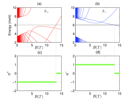
Figure 3: The schematic of evolution of the Chern numbers for each spin component, with increasing the magnetic field in an InAs/GaSb QW system. The model parameters are given in the Table. I. The Fermi energy is fixed at $\mu=6$ meV, as shown by the back lines in (a) and (b). These Chern numbers (c) and (d) are calculated by using Eqs. (16a) and (16b), which is well quantized. The Chern number jumps by +1 ro -1 when the Fermi energy crosses one Landau level.

III.5 Spin Chern numbers and QSHE

Now let us combine the two spin components of $h_{+}$ and $h_{-}$ as a whole system together. As shown in Fig. 2 (c) and (f), developing from the identical gap at zero field for both spin components, there is always a finite region which is just the overlap of their shaded regions, where $h_{+}$ and $h_{-}$ have opposite and nonzero Chern numbers. In this region, the total Hall conductance is zero as a summation of $\sigma_{xy}^{\pm}$, but the spin Hall conductance is still quantized as $\sigma_{s}=[\left(n_{+}-n_{-}\right)/2]\frac{e}{8\pi}=\left[\mathrm{sgn}(B)+\mathrm{sgn}(\Delta)\right]\frac{e}{8\pi}$ even at a finite magnetic field. In other words, the spin Hall conductance in the overlapped region in Fig. 2(c) and (f) remains as that in the absence of the field. This quantum spin Hall conductance $\sigma_{s}$ [or corresponding spin Chern number $n_{s}=\left(n_{+}-n_{-}\right)/2$] is well defined only when there is no coupling between two spin components.

Due to the presence of finite model parameter $B$ (which guarantees $B\cdot\Delta>0$), the envelops separating the conduction and valence bands for $h_{+}$ and $h_{-}$ are not parallel to each other, with the increasing of $\mathcal{B}$. As a result, a topological quantum phase transition occurs when one Landau level from valence band associated with one spin component crosses with that from conduction band associated with another spin component. After this crossing, the Chern numbers associated with the bulk gap maybe not longer opposite to each other, $n_{+}\neq-n_{-}$ for two spin components respectively, making the system from QSHE to other quantum Hall states with both $n=n_{+}+n_{-}\neq 0$ and $n_{s}=n_{+}-n_{-}\neq 0$

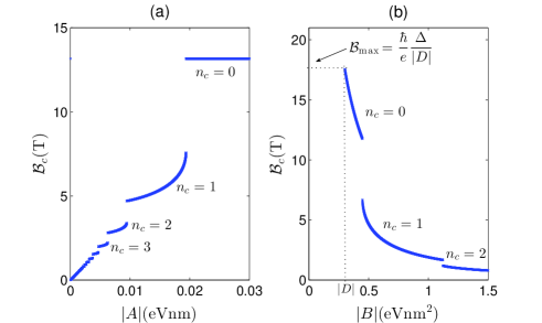
Figure 4: The first crossing magnetic field $\mathcal{B}_{c}$ as a function of model parameters for InAs/GaSb quantum well when other parameters are fixed as in Table.1. (a) $\mathcal{B}_{c}$ as a function of $|A|$. (b) $\mathcal{B}_{c}$ as a function of $|B|$. Different branches correspond to different Landau levels (as indexed) that happen to cross first, starting from low field.

IV Critical magnetic field

We have demonstarted that, the BHZ model (1) displays a well-defined QSHE under a finite magnetic field $\mathcal{B}$, until a band crossing between one conduction band and one valence band from $h_{+}$ and $h_{-}$, respectively, happens at a critical $\mathcal{B}_{c}$. Thus the magnitude of $\mathcal{B}_{c}$ determines the robustness of the QSHE. Now we are in a position to determine this critical magnetic field for various model parameters, with the above knowledge of Landau levels and Chern numbers at finite $\mathcal{B}$. First of all, consider Landau levels with the index $n=0$. Notice there is only one Landau level of $n=0$ from each spin component: the one from $h_{+}$ belongs to the valance band and the one from $h_{-}$ belongs to the conductance band. They always cross at

$$\mathcal{B}_{0}=\dfrac{\hbar}{e}\dfrac{\Delta}{B}$$ (28)

therefore a large ratio between $\Delta$ and $B$ always leads to a large critical value of magnetic field $\mathcal{B}_{0}$. Notice that the gap at $\Gamma$ point is determined by $2\Delta$, not the direct gap away from the $\Gamma$ point. For the model parameters for HgTe and InAs/GaSb quantum wells listed in Table.1, we find that the boundary of the QSHE region is determined by the two levels of $n=0$, and obtain the critical magnetic field $\mathcal{B}_{c}=\mathcal{B}_{0}=$9.59 T and 13.16 T respectively. Such a relatively strong critical magnetic field is consistent with recent experimental observation in InAs/GaSb quantum wellDu-13xxx ; Du2014 .

In a general case, it is also possible for two Landau levels with index $n>0$ to cross first when increasing magnetic field. The general procedure to extract $\mathcal{B}_{c}$ is as follows. It is observed that two definite Landau levels of the sameindex $n>0$ from different spin components will cross first . The general condition to determine the band crossing of two Landau levels with index $n>0$ from $h_{-}$ and $h_{+}$ is given by an integer $n_{c}\leq 1/\sqrt{w(4-w)}$ with $w=A^{2}/[B\Delta(1-D^{2}/B^{2})]$. The corresponding magnetic fields at these crossing points are

$$\mathcal{B}_{c}=\dfrac{\hbar}{e}\frac{n_{c}}{4n_{c}^{2}-1}\dfrac{2\Delta}{B}\left(\zeta-\sqrt{\zeta^{2}-1+\frac{1}{4n_{c}^{2}}}\right),$$ (29)

where $\zeta=1-w$. Since a pair of Landau levels with smaller $n$ crosses at larger $\mathcal{B}$, the first crossing point $\mathcal{B}_{c}$ by increasing the magnetic field is given by the maximal integer $n_{c}$ from the above inequality.

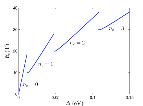
Figure 5: The critical magnetic field $B_{c}$ as a function of $|\Delta|$. Different branches correspond to different Landau levels (as indexed) that happen to cross first.

With this process of determining $\mathcal{B}_{c}$, it is natural to investigate the optimal model parameters for a large critical field, as a guidance for future device fabrication. For a generic group of model parameters, the above process is rather tedious, because of the strongly nonlinear and discontinuous dependence of $\mathcal{B}_{c}$ on these parameters. To extract more insights from Eq. (29), we present the parameter-dependences of the critical magnetic field in Fig. 4 and Fig. 5. The critical field is plotted as a function of the model parameter $A$ in Fig. 4(a). For a sufficiently large $A$, the critical field is determined by the crossing point of two Landau levels of $n_{c}=0$, i.e., $\mathcal{B}_{c}=\dfrac{\hbar}{e}\dfrac{\Delta}{B}$ . When $A$ decreases, $n_{c}$ increases, but the critical field decreases quickly if other parameters remains unchanged. In Fig. 4(b), the critical field increases quickly when the parameter $B$ decreases. The critical field reaches at a maximal value $\mathcal{B}_{c}=\dfrac{\hbar}{e}\dfrac{\Delta}{\left|D\right|}$ when $\left|B\right|\rightarrow\left|D\right|$. We notice that the critical field is very sensitive to model parameters $B$ and $D$, and can be as large as tens of Teslas. As for $\Delta$, as plotted in Fig. 5, the first observation is that the critical field increases with $\Delta$ monotonically for a Landau level crossing with a specific index $n_{c}$. Increasing $\Delta$ leads to a band crossing of Landau levels with a higher index, which corresponds to a larger critical magnetic field $\mathcal{B}_{c}$.

V A perpendicular Zeeman field

The Zeeman coupling can destroy the QSHE in an alternative way. For a perpendicular Zeeman field, the Hamiltonian has an additional term

$$H_{\bot}=V_{\bot}\left(\begin{array}[]{cc}\sigma_{0}&0\\ 0&-\sigma_{0}\end{array}\right),$$ (30)

($\sigma_{0}$ is a $2\times 2$ identity matrix) and $S_{z}$ is still a good quantum number. The main effect of this type of Zeeman coupling to the BHZ model is the change of the gap in $h_{\pm}$:

$$\triangle_{\pm}=\triangle\pm V_{\bot}.$$ (31)

No matter what sign of the gap and the Zeeman field, the Zeeman field always induces a topological transition to a quantum anomalous Hall effect at $\left|V_{\bot}^{c}\right|=\left|\triangle\right|$ according to the formula of the Chern number. When $\left|V_{\bot}^{c}\right|>\left|\triangle\right|$, one is $0$ while another one is $+1$ or $-1$Yu-10science ; Lu-13prl . Thus the total Hall conductance becomes quantized in unit of $e^{2}/h$.

Of course the combined effect of the Zeeman field and the orbital motion may change the critical values of the magnetic field when the $g$ factor is not negligible.

VI Other spin-orbit couplings

So far we just consider the case that two spin-component $h_{+}$ and $h_{-}$ are decoupled such that the spin Chern numbers are well defined. When $S_{z}$ is no longer a good quantum number, the problem becomes more subtle and delicateKonig-08JPSJ . For example, when the Rashba spin-orbit coupling and the Zeeman coupling co-exist in the Kane-Mele model for QSHE, the helical edge states may open a tiny sub-gap Yang-11prl , which clearly indicates the breaking down of the robust quantum spin Hall transport. In the case it is understandable since there is no additional symmetry to protect the QSHE.

The in-plane Zeeman field may couple two spin-components such that we couldn’t calculate the spin Chern numbers as we did in the previous sections. It is still unclear whether or not there exists a hidden symmetry similar to $S_{z}$ after proper transformation such that we could define two “spin”-dependent Chern numbers or the Zeeman coupling is relatively negligible. This will be a subject we need to study further. In the experiment by Du et alDu-13xxx the conductance is quantized while the Fermi level sweeps the whole band gap by tuning the gate voltage. The quantum plateau is also robust up to an 8T perpendicular field and a 12T in-plane magnetic field. Any sub-gap of order of $10^{-3}$meV in the edge states (if exists) should be measurable at low temperatures (tens mK) by sweeping the Fermi level or the gate voltage. One possible explanation is that the Rashba-like spin orbit coupling between $h_{+}$ and $h_{-}$ is negligible, and that the edge states are robust with respect to the $S_{z}$ symmetry. In this case the Chern numbers in $h_{+}$ and $h_{-}$ are still well defined in the presence of a magnetic field. Another possibility is that the strong disorder effect suppresses the spin-orbit coupling. In the experiment the mobility gap and the quantum plateau of conductance coexist, indicating the occurrence of the Anderson localization for the bulk electrons. This is a clear signature of topological Anderson insulator Li-09prl ; Groth-09prl . Thus the disorder may stabilize the QSHE in the system. More studies are expected alone this direction in the future.

In general, when time reversal symmetry is broken, the edge states may open a sub-gap even if there is no bulk band gap closing, which is different from topological quantum phase transition when the symmetry is invariant. For instance the zero end modes in the the Su-Schrieffer-Heeger model with the chirality symmetry move away from the zero energy to the bulk band when a staggered on-site potential is introduced, which breaks the chirality symmetry. In this case the bulk gap never closes even when the end modes move into the bulk bands. This is a key to understand the Thouless charge pumping in the Rice-Mele modelCharge-pump .

VII Summary

In short, the quantum spin Hall effect can persist up to a strong magnetic field when $S_{z}$ is a good quantum number. In this case the spin-dependent Chern number is well defined in each subspace, and according to the bulk-edge correspondenceHatsugai-93prl , the helical edge states are robust to an external field.

References

- (1) J. E. Moore, Nature (London) 464, 194 (2010).
- (2) M. Z. Hasan and C. L. Kane, Rev. Mod. Phys. 82, 3045 (2010).
- (3) X. L. Qi and S. C. Zhang, Rev. Mod. Phys. 83, 1057 (2011).
- (4) S. Q. Shen, Topological Insulators (Springer, Berlin, 2012).
- (5) C. L. Kane and E. J. Mele, Phys. Rev. Lett. 95, 226801(2005).
- (6) B. A. Bernevig, T. L. Hughes, and S. C. Zhang, Science 314, 1757 (2006).
- (7) C. X. Liu, T. L. Hughes, X. L. Qi, K. Wang, and S. C. Zhang, Phys. Rev. Lett. 100, 236601 (2008).
- (8) M. Kï¿œnig, S. Wiedmann, C. Brï¿œne, A. Roth, H. Buhmann, L. W. Molenkamp, X. L. Qi, and S. C. Zhang, Science 318, 766 (2007).
- (9) I. Knez, R. R. Du, and G. Sullivan, Phys. Rev. Lett. 107, 136603 (2011).
- (10) C. L. Kane and E. J. Mele, Phys. Rev. Lett. 95, 146802 (2005).
- (11) L. J. Du, I. Knez, G. Sullivan, and R. R. Du, arXiv: 1306.1925.
- (12) I. Knez, C. T. Rettner, S. H. Yang, S. S. P. Parkin, L. Du, R. R. Du, and G. Sullivan, Phys. Rev. Lett. 112, 026602 (2014).
- (13) C. Xu and J. E. Moore, Phys. Rev. B 73, 045322 (2006).
- (14) C. J. Wu, B. A. Bernevig, and S. C. Zhang, Phys. Rev. Lett. 96, 106401 (2006).
- (15) M. Onoda, Y. Avishai, and N. Nagaosa, Phys. Rev. Lett. 98, 076802 (2007).
- (16) M. Kï¿œnig, H. Buhmann, L. W. Molenkamp, T. Hughes, C. X. Liu, X. L. Qi, and S. C. Zhang, J. Phys. Soc. Jpn. 77, 031007 (2008).
- (17) Y. Y. Yang, Z. Xu, L. Sheng, B. G. Wang, D. Y. Xing and, D. N. Sheng, Phys. Rev. Lett. 107, 066602 (2011).
- (18) B. Zhou, H. Z. Lu, R. L. Chu, S. Q. Shen, and Q. Niu, Phys. Rev. Lett. 101, 246807 (2008).
- (19) H. Z. Lu, W. Y. Shan, W. Yao, Q. Niu, and S. Q. Shen, Phys. Rev. B 81, 115407 (2010).
- (20) D. N. Sheng, Z. Y. Weng, L. Sheng, and F. D. M. Haldane, Phys. Rev. Lett. 97, 036808 (2006).
- (21) S. Q. Shen, M. Ma, X. C. Xie, and F. C. Zhang, Phys. Rev. Lett. 92, 256603 (2004); S. Q. Shen, Y. J. Bao, M. Ma, X. C. Xie, and F. C. Zhang, Phys. Rev. B 71, 155316 (2005)
- (22) R. Yu, W. Zhang, H. J. Zhang, S. C. Zhang, X. Dai, and Z. Fang, Science 329, 61 (2010).
- (23) H. Z. Lu, A. Zhao, and S. Q. Shen, Phys. Rev. Lett. 111, 146802 (2013).
- (24) J. Li, R. L. Chu, J. Jain, and S. Q. Shen, Phys. Rev. Lett. 102, 136806 (2009).
- (25) C. W. Groth, M. Wimmer, A. R. Akhmerov, J. Tworzydlo, and C. W. J. Beenaker, Phys. Rev. Lett. 103, 196805 (2009).
- (26) See Section 4.5 “Thouless charge pump” in Ref. Shen-book, .
- (27) Y. Hatsugai, Phys. Rev. Lett. 71, 3697 (1993).