Sparsity-Aware Sensor Collaboration
for Linear Coherent Estimation

Abstract

In the context of distributed estimation, we consider the problem of sensor collaboration, which refers to the act of sharing measurements with neighboring sensors prior to transmission to a fusion center. While incorporating the cost of sensor collaboration, we aim to find optimal sparse collaboration schemes subject to a certain information or energy constraint. Two types of sensor collaboration problems are studied: minimum energy with an information constraint; and maximum information with an energy constraint. To solve the resulting sensor collaboration problems, we present tractable optimization formulations and propose efficient methods which render near-optimal solutions in numerical experiments. We also explore the situation in which there is a cost associated with the involvement of each sensor in the estimation scheme. In such situations, the participating sensors must be chosen judiciously. We introduce a unified framework to jointly design the optimal sensor selection and collaboration schemes. For a given estimation performance, we empirically show that there exists a trade-off between sensor selection and sensor collaboration.

I Introduction

Wireless sensor networks, consisting of a large number of spatially distributed sensors, have been widely used for applications such as environment monitoring, target tracking and optimal control [1, 2, 3]. In this paper, we study the problem of distributed estimation, where each sensor reports its local observation of the phenomenon of interest and transmits a processed message (after inter-sensor communication) to a fusion center (FC) that determines the global estimate. The act of inter-sensor communication is referred to as sensor collaboration [4], where sensors are allowed to share their raw observations with a set of neighboring nodes prior to transmission to the FC.

In the absence of collaboration, the estimation architecture reduces to a classical distributed estimation network, where scaled versions of sensor measurements are transmitted using an amplify-and-forward strategy [5]. In this setting, one of the key problems is to design the optimal power amplifying factors (i.e., scaling laws) to reach certain design criteria for performance measures, such as estimation distortion and energy cost. Several variations of the conventional distributed estimation problem have been addressed in the literature depending on the quantity to be estimated (random parameter or process) [6, 7], the type of communication (analog-based or quantization-based) [8, 9], nature of transmission channels (coherent or orthogonal) [10, 11] and energy constraints [12].

In the aforementioned literature [5, 6, 7, 8, 9, 10, 11, 12], it is assumed that there is no inter-sensor collaboration. In contrast, here we study the problem of sensor collaboration, which is motivated by a significant improvement of estimation performance resulting from collaboration [4]. Furthermore, in the collaborative estimation system, we consider the energy cost for sensor activation in order to determine the optimal subset of sensors that communicate with the FC. We will derive optimal schemes for sensor selection and collaboration simultaneously.

The problem of sensor collaboration was first proposed in [4] by assuming an orthogonal multiple access channel (MAC) setting with a fully connected network, where all the sensors are allowed to collaborate. It was shown that the optimal strategy is to transmit the processed signal (after collaboration) over the best available channels with power levels consistent with the channel qualities. In [13, 14], a related problem on power allocation was studied for distributed estimation in a sensor network with fixed topologies. This can be interpreted as the problem of sensor collaboration with given network topologies. Recently, the problem of sensor collaboration over a coherent MAC was studied in [15, 16], where it was observed that even a partially connected network can yield performance close to that of a fully connected network, and the problem of sensor collaboration for a family of sparsely connected networks was investigated. Further, the problem of sensor collaboration for estimating a vector of random parameters is studied in [17]. The works [4, 15, 16, 13, 14, 17] assumed that there is no cost associated with collaboration, the collaboration topologies are fixed and given in advance, and the only unknowns are the collaboration weights used to combine sensor observations.

A more relevant reference to this work is our earlier work [18], where the nonzero collaboration cost was taken into account for linear coherent estimation, and a greedy algorithm was developed for seeking the optimal collaboration topology in energy constrained sensor networks. Compared to [18], here we present a non-convex optimization framework to solve the collaboration problem with nonzero collaboration cost. To elaborate, we describe collaboration through a collaboration matrix, in which the nonzero entries characterize the collaboration topology and the values of these entries characterize the collaboration weights. We introduce a formulation that simultaneously optimizes both the collaboration topology and the collaboration weights. In contrast, the optimization in [18] was performed in a sequential manner, where a sub-optimal collaboration topology was first obtained, and then the optimal collaboration weights were sought. The new formulation leads to a more efficient allocation of energy resources as evidenced by improved distortion performance in numerical results.

We study two types of problems while designing optimal collaboration schemes. One is the information constrained collaboration problem, where we minimize the energy cost subject to an information constraint. The other is the energy constrained collaboration problem, where the Fisher information is maximized subject to a total energy budget. Similar formulations have been considered for the problem of power allocation in parameter estimation [5] and state tracking [12, 7]. Characterization of the collaboration cost in this work in terms of the cardinality function, leads to combinatorial optimization problems. For tractability, we employ the reweighted $\ell_{1}$ method [19] and alternating directions method of multipliers (ADMM) [20] to find a locally optimal solution for the information constrained problem. For the energy constrained problem, we exploit its relationship with the information constrained problem and propose a bisection algorithm for its solution. We empirically show that the proposed methods yield near optimal performance.

In the existing collaborative estimation literature [15, 16, 18] with $N$ sensors, it has been assumed that every node can share its information (through the act of collaboration) with other nodes, but only $M$ ($M\leq N$) given nodes have the ability to communicate with the FC. This is due to the fact that it is usually difficult to coordinate multiple sensors for synchronized transmissions to the FC (as required for an amplify-and-forward scheme) and it may not be possible for all the sensors to participate in that process. In this paper, we formalize this notion by adding a finite cost to selecting each particular sensor for coordinated transmissions to the FC. In this way, the total cost may be reduced if only a small number of sensors are selected to transmit their data. For example, a sensor which is far away from the FC may have a higher sensor selection cost [21]. This raises some fundamental questions that we try to answer in the second part of this paper: Which $M$ sensors should be selected? And what is the optimal value of $M$?

It is worth mentioning that the problem of sensor selection has been widely studied in the context of parameter/state estimation, e.g., [22, 23, 24, 25, 26, 27]. In [22], the sensor selection problem for parameter estimation was elegantly formulated with the help of auxiliary Boolean variables, where each Boolean variable determines whether or not its corresponding sensor is selected. In [23], a sparsity-aware sensor selection problem was introduced by minimizing the number of selected sensors subject to a certain estimation quality. In [24, 25, 26], the optimal sensor selection schemes were found by promoting the sparsity of estimator gains. In [27], the design of sensor selection scheme was transformed to the recovery of a sparse matrix. Although both our work and the existing literature [22, 28, 23, 24, 25, 26, 27] use the $\ell_{0}$ norm and $\ell_{1}$ relaxation in dealing with sensor selection problems, our work is significantly different from [22, 28, 23, 24, 25, 26, 27], since the sensor activation scheme is jointly optimized with the collaboration strategy. Once the problem of joint selection and collaboration is solved, we obtain not only the sensor selection scheme but also the collaboration topology and the power allocation scheme for distributed estimation. We emphasize that the focus of the paper is on sensor collaboration where it is employed in conjunction with sensor selection as well as when no sensor selection is involved.

To determine the optimal sensor selection scheme in a collaborative estimation system, we associate (a) the cost of sensor selection with the number of nonzero rows of the collaboration matrix (i.e., its row-sparsity), and (b) the cost of sensor collaboration with the number of nonzero entries of the collaboration matrix (i.e., its overall sparsity). Based on these associations, we then present a unified framework that jointly designs the optimal sensor selection and collaboration schemes. It will be shown that there exists a trade-off between sensor selection and sensor collaboration for a given estimation performance.

In a preliminary version of this paper [29], we presented the optimization framework for designing the optimal sensor collaboration strategy with nonzero collaboration cost and unknown collaboration topologies in scenarios where the set of sensors that communicate with the FC is given in advance. In this paper, we have three new contributions.

• We elaborate on the theoretical foundations of the proposed optimization approaches in [29].

• We improve the computational efficiency of the approaches in [29] by proposing a fast algorithm to solve the resulting optimization problem.

• The issue of sensor selection is taken into account. We present a unified framework for the joint design of optimal sensor selection and collaboration schemes.

The rest of the paper is organized as follows. In Section II, we introduce the collaborative estimation system. In Section III, we formulate the information and energy constrained sensor collaboration problems with non-zero collaboration cost. In Section IV, we develop efficient approaches to solve the information constrained collaboration problem. In Section V, the energy constrained collaboration problem is studied. In Section VI, we investigate the issue of sensor selection. In Section VII, we demonstrate the effectiveness of our proposed framework through numerical examples. Finally, in Section VIII we summarize our work and discuss future research directions.

II Preliminaries: A Model for Sensor Collaboration

In this section, we introduce a distributed estimation system that involves inter-sensor collaboration. We assume that the task of the sensor network is to estimate a random parameter $\theta$, which follows a Gaussian distribution with zero mean and variance $\eta^{2}$. In the estimation system, sensors first report their raw measurements via a linear sensing model. Then, individual sensors can update their observations through spatial collaboration, which refers to (linearly) combining observations from other sensors. The updated measurements are transmitted through a coherent MAC. Finally, the FC determines a global estimate of $\theta$ by using a linear estimator. We show the collaborative estimation system in Fig. 1, and in what follows we elaborate on each of its parts.

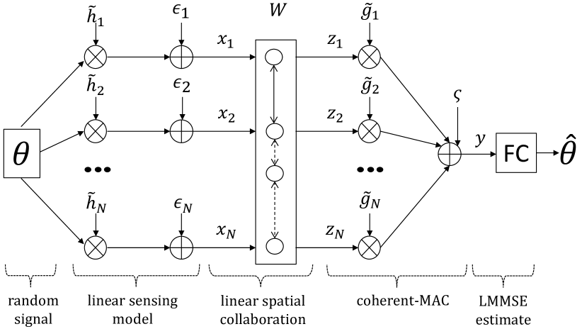
Figure 1: Collaborative estimation architecture showing the sensor measurements, transmitted signals, and the received signal at FC.

The linear sensing model is given by

$$\mathbf{x}=\tilde{\mathbf{h}}\theta+\bm{\epsilon},$$ (1)

where $\mathbf{x}=[x_{1},\ldots,x_{N}]^{T}$ denotes the vector of measurements from $N$ sensors, $\tilde{\mathbf{h}}$ is the vector of observation gains with known second order statistics $\mathbb{E}[\tilde{\mathbf{h}}]=\mathbf{h}$ and $\mathrm{cov}(\tilde{\mathbf{h}})=\bm{\Sigma}_{h}$, and $\bm{\epsilon}$ represents the vector of zero-mean Gaussian noise with $\mathrm{cov}(\bm{\epsilon})=\bm{\Sigma}_{\epsilon}$.

The sensor collaboration process is described by

$$\mathbf{z}=\mathbf{W}\mathbf{x},$$ (2)

where $\mathbf{z}\in\mathbb{R}^{N}$ denotes the message after collaboration, and $\mathbf{W}\in\mathbb{R}^{N\times N}$ is the collaboration matrix that contains weights used to combine sensor measurements. In (2), we assume that sharing of an observation is realized through a reliable (noiseless) communication link that consumes power $C_{mn}$, regardless of its implementation. And the matrix $\mathbf{C}\in\mathbb{R}^{N\times N}$ describing all the collaboration costs among various sensors is assumed to be known in advance. The focus of the present work is on the conceptual aspects of sensor collaboration and not the details of its physical implementation. The proposed ideal and relatively simple collaboration model enables us to readily obtain explicit expressions for the transmission cost and the estimation distortion.

After sensor collaboration, the message $\mathbf{z}$ is transmitted to the FC through a coherent MAC, so that the received signal is a coherent sum [10]

$$y=\tilde{\mathbf{g}}^{T}\mathbf{z}+\varsigma,$$ (3)

where $\tilde{\mathbf{g}}$ is the vector of channel gains with known second order statistics $\mathbb{E}[\tilde{\mathbf{g}}]=\mathbf{g}$ and $\mathrm{cov}(\tilde{\mathbf{g}})=\bm{\Sigma}_{g}$, and $\varsigma$ is a zero-mean Gaussian noise with variance $\xi^{2}$.

The transmission cost is given by the energy required for transmitting the message $\mathbf{z}$ in (2), namely,

$$T_{\mathbf{W}}= ~{}\mathbb{E}_{\theta,\tilde{\mathbf{h}},\bm{\epsilon}}[\mathbf{z}^{T}\mathbf{z}]=\mathbb{E}[\mathbf{x}^{T}\mathbf{W}^{T}\mathbf{W}\mathbf{x}]=\mathbb{E}[\operatorname{tr}(\mathbf{W}\mathbf{x}\mathbf{x}^{T}\mathbf{W}^{T})].$$

From (1), we obtain that

$$\bm{\Sigma}_{x}\mathrel{\mathop{:}}=\mathbb{E}_{\theta,\tilde{\mathbf{h}},\bm{\epsilon}}[\mathbf{x}\mathbf{x}^{T}]=\bm{\Sigma}_{\epsilon}+\eta^{2}(\mathbf{h}\mathbf{h}^{T}+\bm{\Sigma}_{h}).$$ (4)

Thus, the transmission cost can be written as

$$T_{\mathbf{W}}=\operatorname{tr}[\mathbf{W}\bm{\Sigma}_{x}\mathbf{W}^{T}].$$ (5)

We assume that the FC knows the second-order statistics of the observation gain, information gain, and additive noises, and that the corresponding variance and covariance matrices are invertible.

To estimate the random parameter $\theta$, we consider the linear minimum mean square error (LMMSE) estimator [30]

$$\hat{\theta}=a_{\text{\tiny{LMMSE}}}y,$$ (6)

where $a_{\text{\tiny{LMMSE}}}$ is determined by the minimum mean square error criterion. From the theory of linear Bayesian estimators [30], we can readily obtain $a_{\text{\tiny{LMMSE}}}$ and the corresponding estimation distortion

$$a_{\text{\tiny{LMMSE}}}=\operatornamewithlimits{arg\,min}_{a}\mathbb{E}[(\theta-ay)^{2}]=\frac{\mathbb{E}[y\theta]}{\mathbb{E}[y^{2}]},\quad\text{and}$$ (7a)

$$D_{\mathbf{W}}=\mathbb{E}[(\theta-a_{\text{\tiny{LMMSE}}}y)^{2}]=\eta^{2}-\frac{(\mathbb{E}[y\theta])^{2}}{\mathbb{E}[y^{2}]}.$$ (7b)

In (7b), substituting (2) and (3), we obtain

$$\mathbb{E}[y^{2}]= \mathbb{E}[\tilde{\mathbf{g}}^{T}\mathbf{W}\mathbf{x}\mathbf{x}^{T}\mathbf{W}^{T}\tilde{\mathbf{g}}]+\xi^{2}$$

$$= \mathbb{E}[\operatorname{tr}(\tilde{\mathbf{g}}\tilde{\mathbf{g}}^{T}\mathbf{W}\mathbf{x}\mathbf{x}^{T}\mathbf{W}^{T})]=\operatorname{tr}[\bm{\Sigma}_{\tilde{g}}\mathbf{W}\bm{\Sigma}_{x}\mathbf{W}^{T}],$$ (8)

where $\bm{\Sigma}_{\tilde{g}}:=\mathbb{E}[\tilde{\mathbf{g}}\tilde{\mathbf{g}}^{T}]=\mathbf{g}\mathbf{g}^{T}+\bm{\Sigma}_{g}$, and $\bm{\Sigma}_{x}$ is given by (4). Moreover, it is easy to show that

$$\mathbb{E}[y\theta]=\eta^{2}\mathbf{g}^{T}\mathbf{W}\mathbf{h}.$$ (9)

Now, the coefficient of LMMSE estimator $a_{\text{\tiny{LMMSE}}}$ and the corresponding estimation distortion $D_{\mathbf{W}}$ are determined according to (7b), (8) and (9).

We define an equivalent Fisher information $J_{\mathbf{W}}$ which is monotonically related to $D_{\mathbf{W}}$,

$$J_{\mathbf{W}}:= \frac{1}{D_{\mathbf{W}}}-\frac{1}{\eta^{2}}$$

$$= \frac{(\mathbf{g}^{T}\mathbf{W}\mathbf{h})^{2}}{\operatorname{tr}[\bm{\Sigma}_{\tilde{g}}\mathbf{W}\bm{\Sigma}_{x}\mathbf{W}^{T}]-\eta^{2}(\mathbf{g}^{T}\mathbf{W}\mathbf{h})^{2}+\xi^{2}},$$ (10)

For convenience, we often express the estimation distortion (7b) as a function of the Fisher information

$$D_{\mathbf{W}}\mathrel{\mathop{:}}=\frac{\eta^{2}}{1+\eta^{2}J_{\mathbf{W}}}.$$ (11)

III Optimal Sparse Sensor Collaboration

In this section, we first make an association between the collaboration topology and the sparsity structure of the collaboration matrix $\mathbf{W}$. We then define the collaboration cost and sensor selection cost with the help of the cardinality function (also known as the $\ell_{0}$ norm). For simplicity of presentation, we concatenate the elements of $\mathbf{W}$ into a vector form, and present two formulations of collaboration problems (without the cost of sensor selection). By further incorporating the cost of sensor selection, we formulate an optimization problem for the joint design of optimal sensor selection and collaboration schemes.

Recalling the collaboration matrix $\mathbf{W}$ in (2), we note that the nonzero entries of $\mathbf{W}$ correspond to the active collaboration links among sensors. For example, $W_{mn}=0$ indicates the absence of a collaboration link from the $n$th sensor to the $m$th sensor, where $W_{mn}$ is the $(m,n)$th entry of $\mathbf{W}$. Conversely, $W_{mn}\neq 0$ signifies that the $n$th sensor shares its observation with the $m$th sensor. Thus, the sparsity structure of $\mathbf{W}$ characterizes the collaboration topology.

For a given collaboration topology, the collaboration cost is given by

$$Q_{\mathbf{W}}=\sum_{m=1}^{N}\sum_{n=1}^{N}C_{mn}\mathrm{card}(W_{mn}).$$ (12)

where $C_{mn}$ is the cost of sharing an observation from the $n$th sensor to the $m$th sensor. Note that $C_{nn}=0$, since each node can collaborate with itself at no cost. To account for an active collaboration link, we use the cardinality function

$$\mathrm{card}(W_{mn})=\left\{\begin{array}[]{ll}0&\quad W_{mn}=0\\ 1&\quad W_{mn}\neq 0.\end{array}\right.$$ (15)

Next, we define the sensor selection/activation cost. Partitioning the matrix $\mathbf{W}$ rowwise, the linear spatial collaboration process (2) can be written as

$$\begin{bmatrix}z_{1}\\ z_{2}\\ \vdots\\ z_{N}\end{bmatrix}=\mathbf{W}\mathbf{x}=\begin{bmatrix}\bm{\omega}_{1}^{T}\\ \bm{\omega}_{2}^{T}\\ \vdots\\ \bm{\omega}_{N}^{T}\end{bmatrix}\mathbf{x},$$ (16)

where $\bm{\omega}_{n}^{T}$ is the $n$th row vector of $\mathbf{W}$. It is clear from (16) that the non-zero rows of $\mathbf{W}$ characterize the selected sensors that communicate with the FC. Suppose, for example, that only the $n$th sensor communicates with the FC. In this case, it follows from (16) that $z_{n}=\bm{\omega}_{n}^{T}\mathbf{x}$ and $\bm{\omega}_{m}=0$ for $m\neq n$. The goal of sensor selection is to find the best subset of sensors, i.e., $M$ nodes out of a total of $N$ sensor nodes ($M\leq N$), to communicate with the FC. This is in contrast with the existing work [15, 16, 18], where the $M$ communicating nodes are selected a priori.

The sensor selection cost can be defined through the row-wise cardinality of $\mathbf{W}$

$$S_{\mathbf{W}}=\sum_{n=1}^{N}d_{n}\operatorname{card}(\|\bm{\omega}_{n}\|_{2}),$$ (17)

where $\mathbf{d}=[d_{1},d_{2},\ldots,d_{N}]^{T}$ is a given vector of sensor selection cost, and $\|\cdot\|_{2}$ denotes the Euclidean norm (also known as $\ell_{2}$ norm). In (17), the use of $\ell_{2}$ norm is motivated by the problem of group Lasso [31], which uses $\ell_{2}$ norm to promote the group-sparsity of a vector.

Note that both the expressions of transmission cost (5) and Fisher information (10) involve a quadratic matrix function [32]. For simplicity of presentation, we convert the quadratic matrix function to a quadratic vector function, where the elements of $\mathbf{W}$ are concatenated into its row-wise vector $\mathbf{w}$. Specifically, the vector $\mathbf{w}$ is given by

$$\mathbf{w}=[w_{1},w_{2},\ldots,w_{L}]^{T},~{}~{}w_{l}=W_{m_{l}n_{l}},$$ (18)

where $L=N^{2}$, $m_{l}=\lceil\frac{l}{N}\rceil$, $n_{l}=l-(\lceil\frac{l}{N}\rceil-1)N$ and $\lceil x\rceil$ is the ceiling function that yields the smallest integer not less than $x$.

As shown in Appendix A, the expressions of transmission cost (5), Fisher information (10), collaboration cost (12), and selection cost (17) can be converted into functions of the collaboration vector $\mathbf{w}$,

$$T(\mathbf{w})=\mathbf{w}^{T}\bm{\Omega}_{\operatorname*{\text{\tiny{T}}}}\mathbf{w},$$ (19a)

$$J(\mathbf{w})=\frac{\mathbf{w}^{T}\bm{\Omega}_{\text{\tiny{JN}}}\mathbf{w}}{\mathbf{w}^{T}\bm{\Omega}_{\text{\tiny{JD}}}\mathbf{w}+\xi^{2}},$$ (19b)

$$Q(\mathbf{w})=\sum_{l=1}^{L}c_{l}\,\mathrm{card}(w_{l}),\quad$$ (19c)

$$S(\mathbf{w})=\sum_{n=1}^{N}d_{n}\operatorname{card}(\|\mathbf{w}_{\operatorname*{\text{\tiny{G}}}_{n}}\|_{2}),$$ (19d)

where the matrices $\bm{\Omega}_{\operatorname*{\text{\tiny{T}}}}$, $\bm{\Omega}_{\text{\tiny{JN}}}$, $\bm{\Omega}_{\text{\tiny{JD}}}$ are all symmetric positive semidefinite and defined in Appendix A, $c_{l}$ is the $l$th entry of $\mathbf{c}$ that is the row-wise vector of the known cost matrix $\mathbf{C}$, and $\text{G}_{n}$ is an index set such that $\mathbf{w}_{\operatorname*{\text{\tiny{G}}}_{n}}=[w_{(n-1)N+1},w_{(n-1)N+2},\ldots,w_{nN}]^{T}$ for $n=1,2,\ldots,N$. It is clear from (16) and (19d) that the row-sparsity of $\mathbf{W}$ is precisely characterized by the group-sparsity of $\mathbf{w}$ over the index sets $\{\mathrm{G}_{n}\}_{n=1,2,\ldots,N}$.

Based on the transmission cost $T(\mathbf{w})$, collaboration cost $Q(\mathbf{w})$, and performance measure $J(\mathbf{w})$, we first pose the sensor collaboration problems by disregarding the cost of sensor selection and assuming that all $N$ sensors are active.

• Information constrained sensor collaboration

  $$\begin{array}[]{ll}\displaystyle\operatorname*{\text{minimize}}_{\mathbf{w}}&P(\mathbf{w})\\ \operatorname*{\text{subject to}}&J(\mathbf{w})\geq\check{J},\end{array} \mathrm{P}1$$ ()

where

$$P(\mathbf{w})\mathrel{\mathop{:}}=T(\mathbf{w})+Q(\mathbf{w}),$$

and $\check{J}>0$ is a given information threshold.

• Energy constrained sensor collaboration

  $$\begin{array}[]{ll}\displaystyle\operatorname*{\text{maximize}}_{\mathbf{w}}&\displaystyle J(\mathbf{w})\\ \operatorname*{\text{subject to}}&P(\mathbf{w})\leq\hat{P},\end{array} \mathrm{P}2$$ ()

where $\hat{P}>0$ is a given energy budget.

Next, we incorporate the sensor selection cost $S(\mathbf{w})$ in (19d), and pose the optimization problem for the joint design of optimal sensor selection and collaboration schemes.

• Joint sensor selection and collaboration

  $$\begin{array}[]{ll}\displaystyle\operatorname*{\text{minimize}}_{\mathbf{w}}&\displaystyle P(\mathbf{w})+S(\mathbf{w})\\ \operatorname*{\text{subject to}}&\displaystyle J(\mathbf{w})\geq\check{J}.\end{array} \mathrm{P}3$$ ()

In ($\mathrm{P}3$), we minimize the total energy cost subject to an information constraint. This formulation is motivated by scenarios where saving energy is the major goal in the context of sensor selection [33]. Problem ($\mathrm{P}3$) is of a similar form as ($\mathrm{P}1$) except for the incorporation of sensor selection cost. However, we will show that the presence of the sensor selection cost makes finding the solution of ($\mathrm{P}3$) more challenging; see Sec. VI for details.

In ($\mathrm{P}1$)-($\mathrm{P}3$), the cardinality function, which appears in $Q(\mathbf{w})$ and $S(\mathbf{w})$, promotes the sparsity of $\mathbf{w}$, and therefore the sparsity of $\mathbf{W}$. Thus, we refer to ($\mathrm{P}1$)-($\mathrm{P}3$) as sparsity-aware sensor collaboration problems. It is worth mentioning that the proposed sensor collaboration problems are solved in a centralized manner at the FC, whereas the inter-sensor collaboration occurs in a distributed way and among sensors. We also note that ($\mathrm{P}1$)-($\mathrm{P}3$) are nonconvex optimization problems due to the presence of the cardinality function and the nonconvexity of the expression for the Fisher information (see Remark 1). In the following sections, we will elaborate on the optimization approaches for solving ($\mathrm{P}1$)-($\mathrm{P}3$).

IV Information Constrained Sensor Collaboration

In this section, we relax the original information constrained problem ($\mathrm{P}1$) by using an iterative reweighted $\ell_{1}$ minimization method. This results in an $\ell_{1}$ optimization problem, which can be efficiently solved by ADMM.

Due to the presence of the cardinality function, problem ($\mathrm{P}1$) is combinatorial in nature. A state-of-the-art method for solving ($\mathrm{P}1$) is to replace the cardinality function (also referred to as the $\ell_{0}$ norm) with a weighted $\ell_{1}$ norm [19]. This leads to the following optimization problem

$$\begin{array}[]{ll}\displaystyle\operatorname*{\text{minimize}}_{\mathbf{w}}&\mathbf{w}^{T}\bm{\Omega}_{\operatorname*{\text{\tiny{T}}}}\mathbf{w}+\|\bm{\Omega}_{\operatorname*{\text{\tiny{C}}}}\mathbf{w}\|_{1}\\ \operatorname*{\text{subject to}}&\mathbf{w}^{T}(\check{J}\bm{\Omega}_{\text{\tiny{JD}}}-\bm{\Omega}_{\text{\tiny{JN}}})\mathbf{w}+\check{J}\xi^{2}\leq 0,\end{array}$$ (28)

where $\bm{\Omega}_{\operatorname*{\text{\tiny{C}}}}=\operatorname{diag}(\alpha_{1}^{t}c_{1},\alpha_{2}^{t}c_{2},\ldots,\alpha_{L}^{t}c_{L})$, and $\{\alpha_{l}^{t}\}_{l=1,2,\ldots,L}$ denote the weights assigned for entries of an $\ell_{1}$ norm at the $t$th iteration in Algorithm 1. If $\alpha_{l}=1$ for all $l\in\{1,2,\ldots,L\}$, we recover the standard unweighted $\ell_{1}$ norm. Since the $\ell_{0}$ norm only counts the number of nonzero entries of a vector, the use of the $\ell_{1}$ norm for approximating the $\ell_{0}$ norm has the disadvantage that the amplitudes of the nonzero entries come into play. To compensate for the amplitude of nonzero entries, we iteratively normalize the entries of the argument of the $\ell_{1}$ norm, to make this norm a better proxy for the $\ell_{0}$ norm. We summarize the reweighted $\ell_{1}$ method for solving ($\mathrm{P}1$) in Algorithm 1.

Algorithm 1 Reweighted $\ell_{1}$ method for solving ($\mathrm{P}1$)

1:given $\varepsilon>0$ and $\epsilon_{\mathrm{rw}}>0$. Set $\alpha_{l}^{0}=1$ for $l=1,\ldots,L$ and $\bm{\Omega}_{\operatorname*{\text{\tiny{C}}}}=\operatorname{diag}(\alpha_{1}^{0}c_{1},\alpha_{2}^{0}c_{2},\ldots,\alpha_{L}^{0}c_{L})$.

2:for $t=0,1,\ldots$ do

3:     solve problem (28) to obtain solution

4:     $\mathbf{w}^{t}=[w_{1}^{t},w_{2}^{t},\ldots,w_{L}^{t}]^{T}.$

5:     update the weights $\displaystyle\alpha_{l}^{t+1}=\frac{1}{|w_{l}^{t}|+\varepsilon}$ and

6:     $\bm{\Omega}_{\operatorname*{\text{\tiny{C}}}}=\operatorname{diag}(\alpha_{1}^{t+1}c_{1},\alpha_{2}^{t+1}c_{2},\ldots,\alpha_{L}^{t+1}c_{L})$.

7:     if $\|\mathbf{w}^{t+1}-\mathbf{w}^{t}\|_{2}<\epsilon_{\mathrm{rw}}$, quit.

8:end for

Reference [19] shows that much of the benefit of using the reweighted $\ell_{1}$ method is gained from its first few iterations. In Step 3 of Algorithm 1, the positive scalar $\varepsilon$ is a small number which insures that the denominator is always nonzero, and helps the convergence of Algorithm 1; for example, if $w_{l}^{t}\to 0$, the weight $\alpha_{l}^{t+1}$ converges to $\frac{1}{\varepsilon}$.

Remark 1

In (28), the inequality constraint is equivalent to the information inequality in ($\mathrm{P}1$). According to Lemma 2 in Appendix B, we obtain that the matrix $\check{J}\bm{\Omega}_{\operatorname*{\text{\tiny{JD}}}}-\bm{\Omega}_{\operatorname*{\text{\tiny{JN}}}}$ is not positive semidefinite. Indeed, if the matrix $\check{J}\bm{\Omega}_{\operatorname*{\text{\tiny{JD}}}}-\bm{\Omega}_{\operatorname*{\text{\tiny{JN}}}}$ was positive semidefinite, problem (28) would have an empty feasible set.

Given $\{\alpha_{l}^{t}\}_{l=1,\ldots,L}$, problem (28) is a nonconvex optimization problem, and its objective function is not differentiable. In what follows, we will employ ADMM to find its locally optimal solutions.

Alternating Direction Method of Multipliers

In our earlier work [29], we have applied ADMM to solve problem (28). ADMM is an optimization method well-suited for problems that involve sparsity-inducing regularizers (e.g., cardinality function or $\ell_{1}$ norm) [20, 34]. The major advantage of ADMM is that it allows us to split the optimization problem (28) into a nonconvex quadratic program with only one quadratic constraint (QP1QC) and an unconstrained $\ell_{1}$ norm optimization problem, of which the former can be solved efficiently and the latter analytically. When applied to a non-convex problem such as (28), ADMM is not guaranteed to converge and yields locally optimal solutions when it does [20]. However, we have found ADMM to both converge and yield satisfactory results for (28). Indeed, our numerical observations agree with the literature [20, 34, 26] that demonstrates the power and utility of ADMM in solving nonconvex optimization problems.

We begin by reformulating the optimization problem (28) in a way that lends itself to the application of ADMM,

$$\begin{array}[]{ll}\displaystyle\operatorname*{\text{minimize}}_{\mathbf{w},\mathbf{v}}&\mathbf{w}^{T}\bm{\Omega}_{\operatorname*{\text{\tiny{T}}}}\mathbf{w}+\|\bm{\Omega}_{\operatorname*{\text{\tiny{C}}}}\mathbf{v}\|_{1}+\mathcal{I}(\mathbf{w})\\ \operatorname*{\text{subject to}}&\mathbf{w}=\mathbf{v},\end{array}$$ (31)

where we introduce the indicator function $\mathcal{I}(\mathbf{w})$

$$\mathcal{I}(\mathbf{w})=\left\{\begin{array}[]{ll}0&\text{if $\mathbf{w}^{T}(\check{J}\bm{\Omega}_{\text{\tiny{JD}}}-\bm{\Omega}_{\text{\tiny{JN}}})\mathbf{w}+J\xi^{2}\leq 0$}\\ \infty&\text{otherwise}.\end{array}\right.$$ (34)

The augmented Lagrangian of (31) is given by

$$\mathcal{L}(\mathbf{w},\mathbf{v},\bm{\chi})= ~{}\mathbf{w}^{T}\bm{\Omega}_{\text{\tiny{T}}}\mathbf{w}+\|\bm{\Omega}_{\operatorname*{\text{\tiny{C}}}}\mathbf{v}\|_{1}+\mathcal{I}(\mathbf{w})$$

$$~{}+\bm{\chi}^{T}(\mathbf{w}-\mathbf{v})+\frac{\rho}{2}\|\mathbf{w}-\mathbf{v}\|_{2}^{2},$$ (35)

where the vector $\bm{\chi}$ is the Lagrangian multiplier, and the scalar $\rho>0$ is a penalty weight. The ADMM algorithm iteratively executes the following three steps [20] for $k=1,2,\ldots$

$$\mathbf{w}^{k+1} =\operatornamewithlimits{arg\,min}_{\mathbf{w}}~{}\mathcal{L}(\mathbf{w},\mathbf{v}^{k},\bm{\chi}^{k}),$$ (36)

$$\mathbf{v}^{k+1} =\operatornamewithlimits{arg\,min}_{\mathbf{v}}~{}\mathcal{L}(\mathbf{w}^{k+1},\mathbf{v},\bm{\chi}^{k}),$$ (37)

$$\bm{\chi}^{k+1} =\bm{\chi}^{k}+\rho(\mathbf{w}^{k+1}-\mathbf{v}^{k+1}),$$ (38)

until $\|\mathbf{w}^{k+1}-\mathbf{v}^{k+1}\|_{2}\leq\epsilon_{\mathrm{ad}}$ and $\|\mathbf{v}^{k+1}-\mathbf{v}^{k}\|_{2}\leq\epsilon_{\mathrm{ad}}$, where $\epsilon_{\mathrm{ad}}$ is a stopping tolerance.

It is clear from ADMM steps (36)-(37) that the original non-differentiable problem can be effectively separated into a ‘$\mathbf{w}$-minimization’ subproblem (36) and a ‘$\mathbf{v}$-minimization’ subproblem (37), of which the former can be treated as a nonconvex QP1QC and the latter can be solved analytically. In the subsections that follow, we will elaborate on the execution of the minimization problems (36) and (37).

IV-1 $\mathbf{w}$-minimization step

Completing the squares with respect to $\mathbf{w}$ in (35), the $\mathbf{w}$-minimization step (36) is given by

$$\begin{array}[]{ll}\displaystyle\operatorname*{\text{minimize}}_{\mathbf{w}}&\mathbf{w}^{T}\bm{\Omega}_{\text{\tiny{T}}}\mathbf{w}+\frac{\rho}{2}\|\mathbf{w}-\mathbf{a}\|_{2}^{2}\\ \operatorname*{\text{subject to}}&\mathbf{w}^{T}(\check{J}\bm{\Omega}_{\text{\tiny{JD}}}-\bm{\Omega}_{\text{\tiny{JN}}})\mathbf{w}+\check{J}\xi^{2}\leq 0,\end{array}$$ (41)

where we have applied the definition of $\mathcal{I}(\mathbf{w})$ in (34), and $\mathbf{a}\mathrel{\mathop{:}}=\mathbf{v}^{k}-1/\rho\bm{\chi}^{k}$. Problem (41) is a nonconvex QP1QC. To seek the global minimizer of a nonconvex QP1QC, an approach based on semidefinite program (SDP) relaxation has been used in [29]. However, computing solutions to SDP problems becomes inefficient for problems with hundreds or thousands of variables. Therefore, we develop a faster approach by exploiting the KKT conditions of (41). This is presented in Prop. 1.

Proposition 1

The KKT-based solution of problem (41) is given by

$$\mathbf{w}^{k+1}=\tilde{\bm{\Omega}}_{\operatorname*{\text{\tiny{T}}}}^{-\frac{1}{2}}\mathbf{U}\mathbf{u},$$

where $\tilde{\bm{\Omega}}_{\operatorname*{\text{\tiny{T}}}}\mathrel{\mathop{:}}=\bm{\Omega}_{\operatorname*{\text{\tiny{T}}}}+\frac{\rho}{2}\mathbf{I}$, $\mathbf{U}$ is an orthogonal matrix that satisfies the eigenvalue decomposition

$$\frac{1}{\check{J}\xi^{2}}\tilde{\bm{\Omega}}_{\operatorname*{\text{\tiny{T}}}}^{-\frac{1}{2}}(\check{J}\bm{\Omega}_{\text{\tiny{JD}}}-\bm{\Omega}_{\text{\tiny{JN}}})\tilde{\bm{\Omega}}_{\operatorname*{\text{\tiny{T}}}}^{-\frac{1}{2}}=\mathbf{U}\bm{\Lambda}\mathbf{U}^{T},$$ (42)

and $\mathbf{u}$ is given by

$$\left\{\begin{array}[]{ll}\mathbf{u}=-\mathbf{g}&\text{if $\mathbf{g}^{T}\bm{\Lambda}\mathbf{g}+1\leq 0$}\\ \mathbf{u}=-(\mathbf{I}+\mu_{0}\bm{\Lambda})^{-1}\mathbf{g}&\text{otherwise}.\end{array}\right.$$ (45)

In (45), $\mathbf{g}\mathrel{\mathop{:}}=-\frac{\rho}{2}\mathbf{U}^{T}\tilde{\bm{\Omega}}_{\operatorname*{\text{\tiny{T}}}}^{-\frac{1}{2}}\mathbf{a}$, and $\mu_{0}$ is a positive root of the equation in $\mu$

$$f(\mu)\mathrel{\mathop{:}}=\sum_{l=1}^{L}\frac{\lambda_{l}g_{l}^{2}}{(\mu\lambda_{l}+1)^{2}}+1=0,$$ (46)

where $g_{l}$ is the $l$th element of $\mathbf{g}$, and $\lambda_{l}$ is the $l$th diagonal entry of $\bm{\Lambda}$.

Proof: See Appendix C, in which letting $\mathbf{A}_{0}=\tilde{\bm{\Omega}}_{\operatorname*{\text{\tiny{T}}}}$ , $\mathbf{b}_{0}=-\frac{\rho}{2}\mathbf{a}$, $\mathbf{A}_{1}=\check{J}\bm{\Omega}_{\text{\tiny{JD}}}-\bm{\Omega}_{\text{\tiny{JN}}}$, $\mathbf{b}_{1}=\mathbf{0}$ and $r_{1}=\check{J}\xi^{2}$, we can obtain the results given in Prop. 1. $\blacksquare$

The rationale behind deriving the eigenvalue decomposition (42) is that by introducing $\mathbf{u}=\mathbf{U}^{T}\tilde{\bm{\Omega}}_{\operatorname*{\text{\tiny{T}}}}^{\frac{1}{2}}\mathbf{w}$, problem (41) can be transformed to

$$\begin{array}[]{ll}\displaystyle\operatorname*{\text{minimize}}_{\mathbf{u}}&\quad\mathbf{u}^{T}\mathbf{u}+2\mathbf{u}^{T}\mathbf{g}\\ \operatorname*{\text{subject to}}&\quad\mathbf{u}^{T}\bm{\Lambda}\mathbf{u}+1\leq 0.\end{array}$$ (49)

The benefit of this reformulation is that the KKT conditions of (49) are more compact and easily solved, since $\bm{\Lambda}$ is a diagonal matrix and its inversion is tractable. The KKT conditions of (49) are precisely depicted by (45) and (46). We note that solutions of (46) can be found by using the MATLAB function fminbnd or by using Newton’s method.

In general, Eq. (46) is a high-order polynomial function and it is very difficult to obtain all the positive roots. However, we have observed that numerical searches over small targeted intervals yields satisfactory results. One such interval is given by Lemma 3, and the other is demonstrated in Remark 2 below. If we find multiple positive roots, we select the one corresponding to the lowest objective value of the nonconvex QP1QC (41).

Lemma 3: The function $f(\mu)$ is monotonically decreasing on the interval $(0,-\frac{1}{\lambda_{1}})$ and the positive root of $f(\mu)=0$ is unique when $f(0)>0$, where $\lambda_{1}$ represents the unique negative eigenvalue in $\{\lambda_{l}\}_{l=1,2,\ldots,L}$.

Proof: See Appendix D. $\blacksquare$

Remark 2

Motivated by Lemma 3, one may inquire about the monotonicity of $f(\mu)$ over the interval $\mu\in(-\frac{1}{\lambda_{1}},\infty)$. In Appendix D, we show that the sign of the first-order derivative of $f(\mu)$ is difficult to determine from (105) and (106). And our numerical results show that there may exist other positive roots over the interval $(-\frac{1}{\lambda_{1}},\infty)$.

In general, we cannot guarantee global optimality for solutions found through KKT, since KKT conditions constitute only necessary conditions for optimality in nonconvex problems [35]. However, our extensive numerical results show that numerical search over several small intervals works effectively for finding the positive roots of Eq. (46) and the ADMM algorithm always converges to a near-optimal solution of the information constrained collaboration problem.

IV-2 $\mathbf{v}$-minimization step

Completing the squares with respect to $\mathbf{v}$ in (35), the $\mathbf{v}$-minimization step (37) becomes

$$\begin{array}[]{ll}\displaystyle\operatorname*{\text{minimize}}_{\mathbf{v}}&\|\bm{\Omega}_{\operatorname*{\text{\tiny{C}}}}\mathbf{v}\|_{1}+\frac{\rho}{2}\|\mathbf{v}-\mathbf{b}\|_{2}^{2},\end{array}$$ (51)

where $\mathbf{b}\mathrel{\mathop{:}}=\frac{1}{\rho}\bm{\chi}^{k}+\mathbf{w}^{k+1}$. The solution of (51) is given by soft thresholding [34]

$$v_{l}=\left\{\begin{array}[]{cc}(1-\frac{\alpha_{l}^{t}c_{l}}{\rho|b_{l}|})b_{l}&|b_{l}|>\frac{\alpha_{l}^{t}c_{l}}{\rho}\\ 0&|b_{l}|\leq\frac{\alpha_{l}^{t}c_{l}}{\rho}\end{array}\right.$$ (54)

for $l=1,2,\ldots,L$, where $v_{l}$ denotes the $l$th element of the vector $\mathbf{v}$.

IV-3 Initialization

To initialize ADMM we require a feasible vector. It has been shown in Theorem 1 (see Appendix B) that the optimal collaboration vector for a fully-connected network with an information threshold $\check{J}$ is a feasible vector for (28). Thus, we choose $\mathbf{v}^{0}=\mathbf{w}^{0}$ and $\mathbf{w}^{0}=\tilde{\mathbf{w}}$, where $\tilde{\mathbf{w}}$ is given by (95a).

IV-4 Complexity Analysis

To solve the information constrained collaboration problem ($\mathrm{P}1$), the iterative reweighted $\ell_{1}$ method (Algorithm 1) is used as the outer loop, and the ADMM algorithm constitutes the inner loop. It is often the case that the iterative reweighted $\ell_{1}$ method converges within a few iterations [19, 36, 26, 25]. Moreover, it has been shown in [20] that the ADMM algorithm typically requires a few tens of iterations for converging with modest accuracy. At each iteration, the major cost is associated with solving the KKT conditions in the w-minimization step. The complexity of obtaining a KKT-based solution is given by $O(L^{3})$ [37], since the complexity of the eigenvalue decomposition dominates that of Newton’s method.

V Energy Constrained Sensor Collaboration

In this section, we first explore the correspondence between the energy constrained collaboration problem and the information constrained problem. With the help of this correspondence, we propose a bisection algorithm to solve the energy constrained problem.

According to (19a), (19b) and (19c), the energy constrained sensor collaboration problem ($\mathrm{P}2$) can be written as

$$\begin{array}[]{ll}\displaystyle\operatorname*{\text{maximize}}_{\mathbf{w}}&\displaystyle\frac{\mathbf{w}^{T}\bm{\Omega}_{\text{\tiny{JN}}}\mathbf{w}}{\mathbf{w}^{T}\bm{\Omega}_{\text{\tiny{JD}}}\mathbf{w}+\xi^{2}}\\ \operatorname*{\text{subject to}}&\mathbf{w}^{T}\bm{\Omega}_{\operatorname*{\text{\tiny{T}}}}\mathbf{w}+\sum_{l=1}^{L}c_{l}\,\mathrm{card}(w_{l})\leq\hat{P}.\end{array}$$

Compared to the information constrained problem ($\mathrm{P}1$), problem ($\mathrm{P}2$) is more involved due to the nonconvex objective function and the cardinality function in the inequality constraint. Even if we replace the cardinality function with its $\ell_{1}$ norm relaxation, the resulting $\ell_{1}$ optimization problem is still difficult, since the feasibility of the relaxed constraint does not guarantee the feasibility of the original problem ($\mathrm{P}2$).

However, if the collaboration topology is given, the collaboration cost $\sum_{l=1}^{L}c_{l}\,\mathrm{card}(w_{l})$ is a constant and the constraint in ($\mathrm{P}2$) becomes a homogeneous quadratic constraint (i.e., no linear term with respect to $\mathbf{w}$ is involved). In this case, problem ($\mathrm{P}2$) can be solved by [18, Theorem 1].

In Prop 2, we present the relationship between the energy constrained problem ($\mathrm{P}2$) and the information constrained problem ($\mathrm{P}1$). Motivated by this relationship, we then take advantage of the solution of ($\mathrm{P}1$) to obtain the collaboration topology for ($\mathrm{P}2$). This idea will be elaborated on later.

Proposition 2

Consider the two problems ($\mathrm{P}1$) and ($\mathrm{P}2$)

$$\begin{array}[]{ll}\displaystyle\operatorname*{\text{minimize}}_{\mathbf{w}}&P(\mathbf{w})\\ \operatorname*{\text{subject to}}&J(\mathbf{w})\geq\check{J}\end{array}~{}\text{and}~{}\begin{array}[]{ll}\displaystyle\operatorname*{\text{maximize}}_{\mathbf{w}}&J(\mathbf{w})\\ \operatorname*{\text{subject to}}&P(\mathbf{w})\leq\hat{P},\end{array}$$ (59)

where the optimal solutions are denoted by $\mathbf{w}_{1}$ and $\mathbf{w}_{2}$, respectively. If $\check{J}=J(\mathbf{w}_{2})$, then $\mathbf{w}_{1}=\mathbf{w}_{2}$; If $\hat{P}=P(\mathbf{w}_{1})$, then $\mathbf{w}_{2}=\mathbf{w}_{1}$.

Proof: See Appendix E. $\blacksquare$

Prop. 2 implies that the solution of the energy constrained problem ($\mathrm{P}2$) can be obtained by seeking the global minimizer of the information constrained problem ($\mathrm{P}1$), if the information threshold in ($\mathrm{P}1$) is set by using the optimal value of ($\mathrm{P}2$). However, this methodology is intractable in practice since the optimal value of ($\mathrm{P}2$) is unknown in advance, and the globally optimal solution of problem ($\mathrm{P}1$) may not be found using reweighted $\ell_{1}$-based methods.

Instead of deriving the solution of ($\mathrm{P}2$) from ($\mathrm{P}1$), we can infer the collaboration topology of the energy constrained problem ($\mathrm{P}2$) from the sparsity structure of the solution to the information constrained problem ($\mathrm{P}1$) using a bisection algorithm. According to Lemma 1 in Appendix B, the objective function of ($\mathrm{P}2$) (in terms of Fisher information) is bounded over an interval $[0,J_{0})$. And there is a one-to-one correspondence between the value of Fisher information evaluated at the optimal solution of ($\mathrm{P}2$) and energy budget $\hat{P}$. Therefore we perform a bisection algorithm on the interval, and then solve the information constrained problem to obtain the resulting energy cost and collaboration topology. The procedure terminates if the resulting energy cost is close to the energy budget $\hat{P}$. We summarize the bisection algorithm in Algorithm 2.

Algorithm 2 Bisection algorithm for seeking the optimal collaboration topology of ($\mathrm{P}2$)

1:given $\epsilon_{\mathrm{bi}}>0$, $\underline{J}=0$ and $\overline{J}=J_{0}$.

2:repeat$~{}\check{J}=\frac{\underline{J}+\overline{J}}{2}$

3:     for a given $\check{J}$, solve ($\mathrm{P}1$) using Algorithm 1 to obtain      the collaboration topology (in terms of the sparsity      structure of $\mathbf{w}$) and the resulting energy cost $P$.

4:     if $P<\hat{P}$ then $\underline{J}=\check{J}$

5:     else$~{}\overline{J}=\check{J}$

6:     end if

7:until $\overline{J}-\underline{J}<\epsilon_{\mathrm{bi}}$ or $|\hat{P}-P|<\epsilon_{\mathrm{bi}}$

We remark that the collaboration topology obtained in Step 2 of Algorithm 2 is not globally optimal. However, we have observed that for the information constrained sensor collaboration ($\mathrm{P}1$), the value of energy cost $P$ is monotonically related to the value of desired estimation distortion; see Fig. 2 for an example. Therefore, the proposed bisection algorithm converges in practice and at most requires $\lceil\mathrm{log}_{2}(\overline{J}/\epsilon_{\mathrm{bi}})\rceil$ iterations. Once the bisection procedure terminates, we obtain a locally optimal collaboration topology for ($\mathrm{P}2$). Given this topology, the energy constrained problem ($\mathrm{P}2$) becomes a problem with a quadratic constraint and an objective that is a ratio of homogeneous quadratic functions, whose analytical solution is given by [18, Theorem 1]. Through the aforementioned procedure, we obtain a locally optimal solution to problem ($\mathrm{P}2$).

VI Joint Sensor Selection and Collaboration

In this section, we study the problem of the joint design of optimal sensor selection and collaboration schemes, which we formulated in ($\mathrm{P}3$). Similar to solving the information constrained collaboration problem ($\mathrm{P}1$), we first relax the original problem to a nonconvex $\ell_{1}$ optimization problem. However, in contrast to Section IV, we observe that ADMM fails to converge (a possible reason is explored later). To circumvent this, we adopt an iterative method to solve the nonconvex $\ell_{1}$ optimization problem.

Using the reweighted $\ell_{1}$ minimization method, we replace the cardinality function with the weighted $\ell_{1}$ norm, which yields the following $\ell_{1}$ optimization problem at each reweighting iteration

$$\begin{array}[]{ll}\displaystyle\operatorname*{\text{minimize}}_{\mathbf{w}}&\displaystyle\mathbf{w}^{T}\bm{\Omega}_{\operatorname*{\text{\tiny{T}}}}\mathbf{w}+\|\tilde{\bm{\Omega}}_{\operatorname*{\text{\tiny{C}}}}\mathbf{w}\|_{1}+\sum_{n=1}^{N}\tilde{d}_{n}\|\mathbf{w}_{\operatorname*{\text{\tiny{G}}}_{n}}\|_{2}\\ \operatorname*{\text{subject to}}&\mathbf{w}^{T}(\check{J}\bm{\Omega}_{\operatorname*{\text{\tiny{JD}}}}-\bm{\Omega}_{\operatorname*{\text{\tiny{JN}}}})\mathbf{w}+\check{J}\xi^{2}\leq 0,\end{array}$$ (62)

where $\tilde{\bm{\Omega}}_{\operatorname*{\text{\tiny{C}}}}\mathrel{\mathop{:}}=\operatorname{diag}(\tau_{1}^{t}c_{1},\tau_{2}^{t}c_{2},\ldots,\tau_{L}^{t}c_{L})$, $\tilde{d}_{n}\mathrel{\mathop{:}}=\delta_{n}^{t}d_{n}$, $\tau_{l}^{t}$ and $\delta_{n}^{t}$ are the positive weights with respect to $w_{l}$ and $\mathbf{w}_{\operatorname*{\text{\tiny{G}}}_{n}}$ at the reweighting iteration $t$, respectively. Let the solution of (62) be $\mathbf{w}^{t}$, then the weights $\tau_{l}^{t+1}$ and $\delta_{n}^{t+1}$ for the next reweighting iteration are updated as

$$\tau_{l}^{t+1}=\frac{1}{|w_{l}^{t}|+\varepsilon},~{}~{}\delta_{n}^{t+1}=\frac{1}{\|\mathbf{w}_{\operatorname*{\text{\tiny{G}}}_{n}}^{t}\|_{2}+\varepsilon},$$

where we recall that $\varepsilon$ is a small positive number that insures a nonzero denominator.

VI-A Convex restriction

Problem (62) is a nonconvex optimization problem. Similar to our approach in Section IV to find solutions of (28), one can use ADMM to split (62) into a nonconvex QP1QC ($\mathbf{w}$-minimization step) and an unconstrained optimization problem with an objective function composed of $\ell_{1}$ and $\ell_{2}$ norms ($\mathbf{v}$-minimization step), where the latter can be solved analytically. However, our numerical examples show that the resulting ADMM algorithm fails to converge. Note that in the $\mathbf{w}$-minimization step, the sensor selection cost is excluded and each sensor collaborates with itself at no cost. Therefore, to achieve an information threshold, there exist scenarios in which the collaboration matrix yields nonzero diagonal entries. This implies that the $\mathbf{w}$-minimization step does not produce group-sparse solutions (i.e., row-wise sparse collaboration matrices). However, the $\mathbf{v}$-minimization step always leads to group-sparse solutions. The mismatched sparsity structures of solutions in the subproblems of ADMM cause the issue of nonconvergence, which we circumvent by using a linearization method to convexify the optimization problem.

A linearization method is introduced in [38] for solving the nonconvex quadratically constrained quadratic program (QCQP) by linearizing the nonconvex parts of quadratic constraints, thus rendering a convex QCQP. In (62), the nonconvex constraint is given by

$$\mathbf{w}^{T}\check{J}\bm{\Omega}_{\operatorname*{\text{\tiny{JD}}}}\mathbf{w}+\check{J}\xi^{2}\leq\mathbf{w}^{T}\bm{\Omega}_{\operatorname*{\text{\tiny{JN}}}}\mathbf{w},$$ (63)

where $\bm{\Omega}_{\operatorname*{\text{\tiny{JD}}}}$ and $\bm{\Omega}_{\operatorname*{\text{\tiny{JN}}}}$ are positive semidefinite; see (89)-(94). We linearize the right hand side of (63) around a feasible point $\bm{\beta}$

$$\mathbf{w}^{T}\check{J}\bm{\Omega}_{\operatorname*{\text{\tiny{JD}}}}\mathbf{w}+\check{J}\xi^{2}\leq{\bm{\beta}}^{T}\bm{\Omega}_{\operatorname*{\text{\tiny{JN}}}}\bm{\beta}+2{\bm{\beta}}^{T}\bm{\Omega}_{\operatorname*{\text{\tiny{JN}}}}(\mathbf{w}-\bm{\beta}).$$ (64)

Note that the right hand side of (64) is an affine lower bound on the convex function $\mathbf{w}^{T}\bm{\Omega}_{\operatorname*{\text{\tiny{JN}}}}\mathbf{w}$. This implies that the set of $\mathbf{w}$ that satisfy (64) is a strict subset of the set of $\mathbf{w}$ that satisfy (63).

By replacing (63) with (64), we obtain a ‘restricted’ convex version of problem (62)

$$\begin{array}[]{ll}\displaystyle\operatorname*{\text{minimize}}_{\mathbf{w}}&\displaystyle\varphi(\mathbf{w})\mathrel{\mathop{:}}=\mathbf{w}^{T}\bm{\Omega}_{\operatorname*{\text{\tiny{T}}}}\mathbf{w}+\|\tilde{\bm{\Omega}}_{\operatorname*{\text{\tiny{C}}}}\mathbf{w}\|_{1}+\sum_{n=1}^{N}\tilde{d}_{n}\|\mathbf{w}_{\operatorname*{\text{\tiny{G}}}_{n}}\|_{2}\\ \operatorname*{\text{subject to}}&\mathbf{w}^{T}\tilde{\bm{\Omega}}_{\operatorname*{\text{\tiny{JD}}}}\mathbf{w}-2\tilde{\bm{\beta}}^{T}\mathbf{w}+\tilde{\gamma}\leq 0,\end{array}$$ (67)

where $\tilde{\bm{\Omega}}_{\operatorname*{\text{\tiny{JD}}}}\mathrel{\mathop{:}}=\check{J}\bm{\Omega}_{\operatorname*{\text{\tiny{JD}}}}$, $\tilde{\bm{\beta}}\mathrel{\mathop{:}}=\bm{\Omega}_{\operatorname*{\text{\tiny{JN}}}}\bm{\beta}$, and $\tilde{\gamma}\mathrel{\mathop{:}}={\bm{\beta}}^{T}\bm{\Omega}_{\operatorname*{\text{\tiny{JN}}}}\bm{\beta}+\check{J}\xi^{2}$. Different from (63), the inequality constraint in (67) no longer represents the information inequality but becomes a convex quadratic constraint. Since problem (67) is convex, the convergence of ADMM is now guaranteed [20]. And the optimal value of (67) yields an upper bound on that of (62).

We summarize the linearization method in Algorithm 3. In the following subsection, we will elaborate on the implementation of ADMM in Step 3 of Algorithm 3. We remark that the convergence of Algorithm 3 is guaranteed [38], since Algorithm 3 starts from a feasible point $\mathbf{w}^{0}$ that satisfies (63) and at each iteration, we solve a linearized convex problem with a smaller feasible set which contains the linearization point (i.e., the solution at the previous iteration). In other words, for a given linearization point $\bm{\beta}=\mathbf{w}^{s-1}$, we always obtain a new feasible point $\mathbf{w}^{s}$ with a lower or equal objective value at each iteration. Finally, we note that the iterative algorithm can be initialized at $\tilde{\mathbf{w}}$, which is given by (95a).

Algorithm 3 Linearization method on solving (62)

1:given $\epsilon_{\mathrm{li}}>0$ and $\mathbf{w}^{0}=\tilde{\mathbf{w}}$.

2:for iteration $s=1,2,\ldots$ do

3:     set $\bm{\beta}=\mathbf{w}^{s-1}$.

4:     solve (67) for the solution $\mathbf{w}^{s}$ by using Algorithm 4.

5:     until $\|\varphi(\mathbf{w}^{s})-\varphi(\mathbf{w}^{s-1})\|<\epsilon_{\mathrm{li}}$.

6:end for

VI-B Solution via ADMM

Similar to (31) in Sec. IV, we introduce the auxiliary variable $\mathbf{v}$ to replace $\mathbf{w}$ in the $\ell_{1}$ and $\ell_{2}$ norms in (67) while adding the constraint $\mathbf{w}=\mathbf{v}$, and split problem (67) into a sequence of subproblems as in (36)-(38). However, compared to Sec. IV, the current ADMM algorithm yields different subproblems due to the presence of the $\ell_{2}$ norm in the objective function and the convexification in the constraint.

VI-B1 $\mathbf{w}$-minimization step

According to (36), the $\mathbf{w}$-minimization step is given by

$$\begin{array}[]{ll}\displaystyle\operatorname*{\text{minimize}}_{\mathbf{w}}&\mathbf{w}^{T}\tilde{\bm{\Omega}}_{\operatorname*{\text{\tiny{T}}}}\mathbf{w}-\rho\mathbf{a}^{T}\mathbf{w}\\ \operatorname*{\text{subject to}}&\mathbf{w}^{T}\tilde{\bm{\Omega}}_{\operatorname*{\text{\tiny{JD}}}}\mathbf{w}-2\tilde{\bm{\beta}}^{T}\mathbf{w}+\tilde{\gamma}\leq 0,\end{array}$$ (70)

where $\tilde{\bm{\Omega}}_{\operatorname*{\text{\tiny{T}}}}=\bm{\Omega}_{\operatorname*{\text{\tiny{T}}}}+\frac{\rho}{2}\mathbf{I}$, $\mathbf{a}=\mathbf{v}^{k}-1/\rho\bm{\chi}^{k}$, $\mathbf{v}^{k}$ and $\bm{\chi}^{k}$ denote the value of $\mathbf{v}$ and $\bm{\chi}$ at the $k$th iteration of ADMM, and $\bm{\chi}$ is the dual variable. Note that different from problem (41), problem (70) is a convex QCQP, which can be efficiently solved.

To solve the convex QCQP (70), the complexity of using interior-point method in standard solvers is roughly $O(L^{3.5})$ [39]. To reduce the computational complexity, we can derive the KKT-based solution of (70). Since problem (70) is convex, KKT conditions are both necessary and sufficient for optimality. Similar to Prop. 1, we can apply the eigenvalue decomposition technique to simplify (70) and find its solution. This is summarized in Prop. 3.

Proposition 3

The optimal solution of problem (70) is given by

$$\mathbf{w}^{k+1}={\tilde{\bm{\Omega}}_{\operatorname*{\text{\tiny{T}}}}}^{-\frac{1}{2}}{\mathbf{U}}{\mathbf{u}},$$

where ${\mathbf{U}}$ is given by the following eigenvalue decomposition

$$\frac{1}{\tilde{\gamma}}{\tilde{\bm{\Omega}}_{\operatorname*{\text{\tiny{T}}}}}^{-\frac{1}{2}}\tilde{\bm{\Omega}}_{\operatorname*{\text{\tiny{JD}}}}\tilde{\bm{\Omega}}_{\operatorname*{\text{\tiny{T}}}}^{-\frac{1}{2}}={\mathbf{U}}{\bm{\Lambda}}{\mathbf{U}}^{T},$$

and ${\mathbf{u}}$ is given by

$$\left\{\begin{array}[]{ll}{\mathbf{u}}=-{\mathbf{g}}&\text{if ${\mathbf{g}}^{T}{\bm{\Lambda}}{\mathbf{g}}+2{\mathbf{g}}^{T}{\mathbf{e}}+1\leq 0$}\\ {\mathbf{u}}=-(\mathbf{I}+\mu_{1}{\bm{\Lambda}})^{-1}({\mathbf{g}}+\mu_{1}{\mathbf{e}})&\text{otherwise}.\end{array}\right.$$ (73)

In (73), ${\mathbf{g}}=-\rho{\mathbf{U}}^{T}\tilde{\bm{\Omega}}_{\operatorname*{\text{\tiny{T}}}}^{-\frac{1}{2}}\mathbf{a}/2$, ${\mathbf{e}}=-{\mathbf{U}}^{T}\tilde{\bm{\Omega}}_{\operatorname*{\text{\tiny{T}}}}^{-\frac{1}{2}}\tilde{\bm{\beta}}/{\tilde{\gamma}}$, $\mu_{1}$ is the positive root of the equation in $\mu$

$$\sum_{l=1}^{L}\frac{(\lambda_{l}g_{l}-e_{l})^{2}}{\lambda_{l}(1+\mu\lambda_{l})^{2}}-\sum_{l=1}^{L}\frac{e_{l}^{2}}{\lambda_{l}}+1=0,$$

$e_{l}$ and $g_{l}$ are the $l$th elements of $\mathbf{e}$ and $\mathbf{g}$, respectively, and $\lambda_{l}$ is the $l$th diagonal entry of $\bm{\Lambda}$.

Proof: See Appendix C, in which letting $\mathbf{A}_{0}=\tilde{\bm{\Omega}}_{\operatorname*{\text{\tiny{T}}}}$,$\mathbf{b}_{0}=-\frac{\rho}{2}\mathbf{a}$, $\mathbf{A}_{1}=\tilde{\bm{\Omega}}_{\operatorname*{\text{\tiny{JD}}}}$, $\mathbf{b}_{1}=-\tilde{\bm{\beta}}$ and $r_{1}=\tilde{\gamma}$, we obtain the result in Prop. 3. $\blacksquare$

We remark that Prop. 3 is similar to Prop. 1 except for the presence of $\mathbf{e}$ and positive eigenvalues $\{\lambda_{l}\}_{l=1,2,\ldots,L}$. These difference are caused by the convex restriction of (62).

VI-B2 $\mathbf{v}$-minimization step

According to (37), the $\mathbf{v}$-minimization step is given by

$$\begin{array}[]{ll}\displaystyle\operatorname*{\text{minimize}}_{\mathbf{v}}&\displaystyle\|\tilde{\bm{\Omega}}_{\operatorname*{\text{\tiny{C}}}}\mathbf{v}\|_{1}+\sum_{n=1}^{N}\tilde{d}_{n}\|\mathbf{v}_{\operatorname*{\text{\tiny{G}}}_{n}}\|_{2}+\frac{\rho}{2}\|\mathbf{v}-\mathbf{b}\|_{2}^{2},\end{array}$$ (75)

where $\mathbf{b}=\mathbf{w}^{k+1}+1/\rho\bm{\chi}^{k}$.

We recall that $\tilde{\bm{\Omega}}_{\operatorname*{\text{\tiny{C}}}}$ defined in (62) is a diagonal matrix. Let the vector $\mathbf{f}$ be composed of the diagonal entries of $\tilde{\bm{\Omega}}_{\operatorname*{\text{\tiny{C}}}}$. We then define a sequence of diagonal matrices $\mathbf{F}_{n}:=\operatorname{diag}(\mathbf{f}_{\operatorname*{\text{\tiny{G}}}_{n}})$ for $n=1,2,\ldots,N$, where $\mathbf{f}_{\operatorname*{\text{\tiny{G}}}_{n}}$ is a vector composed of those entries of $\mathbf{f}$ whose indices belong to the set $\mathrm{G}_{n}$. Since the index sets $\{\mathrm{G}_{n}\}_{j=1,2,\ldots,N}$ are disjoint, problem (75) can be decomposed into a sequence of subproblems for $n=1,2,\ldots,N$,

$$\begin{array}[]{ll}\displaystyle\operatorname*{\text{minimize}}_{\mathbf{v}_{\operatorname*{\text{\tiny{G}}}_{n}}}&\displaystyle\|\mathbf{F}_{n}\mathbf{v}_{\operatorname*{\text{\tiny{G}}}_{n}}\|_{1}+\tilde{d}_{n}\|\mathbf{v}_{\operatorname*{\text{\tiny{G}}}_{n}}\|_{2}+\frac{\rho}{2}\|\mathbf{v}_{\operatorname*{\text{\tiny{G}}}_{n}}-\mathbf{b}_{\operatorname*{\text{\tiny{G}}}_{n}}\|_{2}^{2}.\end{array}$$ (77)

Problem (77) can be solved analytically via the following proposition.

Proposition 4

The minimizer of (77) is given by

$$\mathbf{v}_{\operatorname*{\text{\tiny{G}}}_{n}}=\left\{\begin{array}[]{cl}(1-\frac{\tilde{d}_{n}}{\rho\|\bm{\nu}\|_{2}})\bm{\nu}&\quad\|\bm{\nu}\|_{2}\geq\frac{\tilde{d}_{n}}{\rho}\vspace*{0.05in}\\ 0&\quad\|\bm{\nu}\|_{2}<\frac{\tilde{d}_{n}}{\rho},\end{array}\right.$$ (80)

where $\bm{\nu}=\mathrm{sgn}(\mathbf{b}_{\operatorname*{\text{\tiny{G}}}_{n}})\odot\mathrm{max}(|\mathbf{b}_{\operatorname*{\text{\tiny{G}}}_{n}}|-\frac{1}{\rho}\mathbf{f}_{\operatorname*{\text{\tiny{G}}}_{n}},0),$ the operator $\mathrm{sgn}(\cdot)$ is defined in a componentwise fashion as

$$\mathrm{sgn}(x)=\left\{\begin{array}[]{l l}1&x>0\\ 0&x=0\\ -1&x<0,\end{array}\right.$$

$\odot$ denotes the point-wise product, and the operator $\mathrm{max}(\mathbf{x},\mathbf{y})$ returns a vector whose entries are the pointwise maximum of the entries of $\mathbf{x}$ and $\mathbf{y}$.

Proof: The main idea of the proof, motivated by [40, Theorem 1], is to study the subgradient of a nonsmooth objective function. However, for problem (77), we require to exploit its particular features: weighted $\ell_{1}$ norm $\|\tilde{\bm{\Omega}}_{\operatorname*{\text{\tiny{C}}}}\mathbf{v}\|_{1}$, and disjoint sub-vectors $\{\mathbf{v}_{\operatorname*{\text{\tiny{G}}}_{n}}\}_{n=1,2,\ldots,N}$. See Appendix F for the complete proof. $\blacksquare$

In Algorithm 4, we present our proposed ADMM algorithm for solving (67).

Algorithm 4 Solving problem (67) via ADMM

1:given $\rho$, $\epsilon_{\mathrm{ad}}$, $\bm{\chi}^{0}=\mathbf{0}$ and $\mathbf{w}^{0}=\mathbf{v}^{0}=\tilde{\mathbf{w}}$.

2:for $k=0,1,\ldots$ do

3:     obtain $\mathbf{w}^{k+1}$ from a standard QCQP solver or Prop. 3.

4:     obtain $\mathbf{v}^{k+1}=[(\mathbf{v}_{\operatorname*{\text{\tiny{G}}}_{1}}^{k+1})^{T},\ldots,(\mathbf{v}_{\operatorname*{\text{\tiny{G}}}_{N}}^{k+1})^{T}]^{T}$ from Prop. 4.

5:     update dual variable $\bm{\chi}^{k+1}=\bm{\chi}^{k}+\rho(\mathbf{w}^{k+1}-\mathbf{v}^{k+1}).$

6:     until $\|\mathbf{w}^{k+1}-\mathbf{v}^{k+1}\|_{2}\leq\epsilon_{\mathrm{ad}},~{}\|\mathbf{v}^{k+1}-\mathbf{v}^{k}\|_{2}\leq\epsilon_{\mathrm{ad}}$.

7:end for

To summarize, for solving the original problem ($\mathrm{P}3$) we first replace the cardinality function with the weighted $\ell_{1}$ norm, which yields the nonconvex problem (62). We then use the linearization method to convexify (62). The resulting convex problem (67) is solved by ADMM as outlined in Algorithm 4.

VII Numerical Results

In this section, we will illustrate the performance of our proposed sparsity-aware sensor collaboration methods through numerical examples. The estimation system considered here is shown in Fig.1, where for simplicity, we assume that the channel gain and uncertainties are such that the network is homogeneous and equicorrelated. As in [18, Example 3], we denote the expected observation and channel gains by $h_{0}$ and $g_{0}$, the observation and channel gain uncertainties by $\alpha_{h}$ and $\alpha_{g}$, the measurement noise variance and correlation by $\zeta^{2}$ and $\rho_{\mathrm{corr}}$, and thereby assume

$$\left\{\begin{array}[]{l}\mathbf{h}=h_{0}\sqrt{\alpha_{h}}\mathbf{1},~{}\bm{\Sigma}_{h}=h_{0}^{2}(1-\alpha_{h})\mathbf{I},\\ \bm{\Sigma}_{\epsilon}=\zeta^{2}[(1-\rho_{\mathrm{corr}})\mathbf{I}+\rho_{\mathrm{corr}}\mathbf{1}\mathbf{1}^{T}],\\ \mathbf{g}=g_{0}\sqrt{\alpha_{g}}\mathbf{1},~{}\bm{\Sigma}_{g}=g_{0}^{2}(1-\alpha_{g})\mathbf{I}.\end{array}\right.$$ (84)

Note that channel gains can also be calculated based on path loss models [41] but we chose the homogeneous model for the sake of simplicity. The collaboration cost matrix $\mathbf{C}$ is given by

$$C_{mn}=\alpha_{\mathrm{c}}\|\mathbf{s}_{m}-\mathbf{s}_{n}\|_{2}$$ (85)

for $m,n=1,2,\ldots,N$, where $\alpha_{\mathrm{c}}$ is a positive parameter and $\mathbf{s}_{n}$ denotes the location of sensor $n$. The vector of sensor selection cost $\mathbf{d}$ is give by

$$d_{n}=\alpha_{\mathrm{s}}\|\mathbf{s}_{n}-\mathbf{s}_{\mathrm{fc}}\|_{2}$$ (86)

for $n=1,2,\ldots,N$, where $\alpha_{\mathrm{s}}$ is a positive parameter and $\mathbf{s}_{\mathrm{fc}}$ denotes the location of the FC.

In our experiments, unless specified otherwise, we shall assume that $h_{0}=g_{0}=1$, $\alpha_{h}=\alpha_{g}=0.7$, $\rho_{\mathrm{corr}}=0.5$, $\xi^{2}=\zeta^{2}=1$, $\eta^{2}=0.1$, and $\alpha_{\mathrm{c}}=\alpha_{\mathrm{s}}=0.01$. The FC and $N$ sensors are randomly deployed on a $10\times 10$ grid, where the value of $N$ will be specified in different examples. While employing the proposed optimization methods, we select $\rho\geq 20$ in ADMM, $\varepsilon=10^{-3}$ in the reweighted $\ell_{1}$ method and $\epsilon_{\mathrm{rw}}=\epsilon_{\mathrm{bi}}=\epsilon_{\mathrm{li}}=\epsilon_{\mathrm{ad}}=10^{-3}$ for the stopping tolerance. In our numerical examples, the reweighted $\ell_{1}$ method (Algorithm 1), the bisection algorithm (Algorithm 2) and the linearization method (Algorithm 3) converge within $10$ iterations. For ADMM, the required number of iterations is less than $100$.

For a better depiction of estimation performance, since $D_{0}<D_{\mathbf{w}}\leq\eta^{2}$ (see Lemma 1 in Appendix B), we display the normalized distortion

$$D_{\mathrm{norm}}:=\frac{D(\mathbf{w})-D_{0}}{\eta^{2}-D_{0}}\in(0,1],$$ (87)

where $D(\mathbf{w})$ defined in (11) is monotonically related to the value of Fisher information, and $D_{0}$ is the minimum estimation distortion given by Lemma 1. Further to characterize the number of established collaboration links, we define the percentage of collaboration links

$$\mathrm{Per}_{\mathbf{w}}:=\frac{\sum_{l=1}^{L}\mathrm{card}(w_{l})-N}{L-N}\times 100~{}~{}(\%),$$ (88)

where $L=N^{2}$ is the dimension of $\mathbf{w}$, and $\mathrm{Per}_{\mathbf{w}}$ belongs to $[0,100\%]$. When $\mathrm{Per}_{\mathbf{w}}=0$, the network operates in a distributed manner (i.e., only the diagonal entries of $\mathbf{W}$ are nonzero). When $\mathrm{Per}_{\mathbf{w}}=100\%$, the network is fully-connected (i.e., $\mathbf{W}$ has no zero entries).

Figure 2: Performance evaluation for information constrained sensor collaboration.

(a) (b) (c)

Figure 3: Information constrained collaboration for different values of collaboration cost parameter $\alpha_{\mathrm{c}}$ as $D_{\mathrm{norm}}\in\{0.05,0.1,0.2\}$: (a) percentage of collaboration links, (b) transmission cost, (c) trade-off between collaboration links and transmission cost.

(a) (b) (c)

Figure 4: Collaboration topologies: (a) $\alpha_{\mathrm{c}}=5\times 10^{-3}$, $\mathrm{card}(\mathbf{w})=18$; (b) $\alpha_{\mathrm{c}}=10^{-3}$, $\mathrm{card}(\mathbf{w})=39$; (c) $\alpha_{\mathrm{c}}=2\times 10^{-4}$, $\mathrm{card}(\mathbf{w})=70$.

In Fig. 2, we present results when we apply the reweighted $\ell_{1}$-based ADMM algorithm to solve the information constrained problem ($\mathrm{P}1$). For comparison, we also show the results of using an exhaustive search that enumerates all possible sensor collaboration schemes, where for the tractability of an exhaustive search, we consider a small sized sensor network with $N=5$. In the top subplot of Fig. 2, we present the minimum energy cost as a function of $D_{\mathrm{norm}}$. We can see that the energy cost and estimation distortion is monotonically related, and the proposed approach assures near optimal performance compared to the results of exhaustive search. In the bottom subplot, we show the number of active collaboration links as a function of normalized distortion. Note that a larger estimation distortion corresponds to fewer collaboration links.

In Fig. 3, we solve the information constrained problem for a relatively large network with $N=10$ nodes, and present the number of collaboration links and the required transmission cost as a function of the collaboration cost parameter $\alpha_{\mathrm{c}}$ for different values of estimation distortion $D_{\mathrm{norm}}\in\{0.05,0.1,0.2\}$. Fig. 3-(a) shows that the number of collaboration links increases as $\alpha_{\mathrm{c}}$ decreases. This is expected, since a smaller value of $\alpha_{\mathrm{c}}$ corresponds to a smaller cost of sensor collaboration, and thus encourages a larger number of collaboration links to be established. If we fix the value of $\alpha_{\mathrm{c}}$, we also observe that the number of collaboration links increases as $D_{\mathrm{norm}}$ decreases. This is consistent with the results in the bottom subplot of Fig 2. We show the specific collaboration topologies that correspond to the marked values of $\alpha_{c}$ in Fig. 4. These will be discussed in detail later.

Fig. 3-(b) shows that the transmission cost increases as $\alpha_{\mathrm{c}}$ increases for a given estimation distortion. Note that a larger value of $\alpha_{\mathrm{c}}$ indicates a higher cost of sensor collaboration. Therefore, to achieve a certain estimation performance, more transmission cost would be consumed instead of sensor collaboration. This implies that the transmission cost and collaboration cost are two conflicting terms. As we continue to increase $\alpha_{\mathrm{c}}$, the transmission cost converges to a fixed value for a given $D_{\mathrm{norm}}$. This is because the network topology cannot be changed any further (converges to the distributed network), where the transmission cost is deterministic for the given topology and distortion.

Fig. 3-(c) shows the trade-off between the number of collaboration links and the consumed transmission cost by varying the parameter $\alpha_{\mathrm{c}}$. One interesting observation is that the transmission cost ceases to decrease significantly when over $50\%$ collaboration links are established. The reason is that the transmission cost is characterized by the magnitude of nonzero entries in $\mathbf{w}$, which has very small increment as the number of active links is relatively large.

In Fig. 4, we present the collaboration topologies obtained from solutions of the information constrained problem (with $D_{\mathrm{norm}}=0.2$) by varying the parameter of collaboration cost $\alpha_{\mathrm{c}}$; see the labeled points in Fig. 3-(a). In each subplot, the solid lines with arrows represent the collaboration links among local sensors. For example in Fig. 4-(a), the line from sensor $1$ to sensor $4$ indicates that sensor $1$ shares its observation with sensor $4$. Fig. 4-(a) shows that the nearest neighboring sensors collaborate initially because of the lower collaboration cost. We continue to decrease $\alpha_{\mathrm{c}}$, Fig. 4-(c) and (d) show that more collaboration links are established, and sensors tends to collaborate over the entire spatial field rather than aggregating in a small neighbourhood.

Figure 5: Transmission cost and collaboration link percentage versus the ratio of measurement noise power and channel noise power.

In Fig. 5, we solve the information constrained problem with $N=10$ and $D_{\text{norm}}\in\{0.05,0.08,0.1\}$ to demonstrate the power allocation schemes when the ratio $\frac{\zeta^{2}}{\xi^{2}}$ of measurement noise power to channel noise power varies. In the top plots of Fig. 5, we present the transmission cost which is normalized over the obtained total energy cost. Given a value of $D_{\text{norm}}$, we observe that when the measurement noise power is much less than the channel noise power, the transmission cost dominates the total energy cost since transmission over noisy channels requires more transmission power. Conversely, when the measurement noise power is much larger than the channel noise power, most of the energy is allocated for sensor collaboration. This is because the act of sensor collaboration can be regarded as a kind of local averaging that effectively reduces the measurement uncertainty at each node. If we fix the ratio of noise power $\frac{\zeta^{2}}{\xi^{2}}$, we note that to improve the estimation performance, more transmission and collaboration power are consumed.

Figure 6: Performance evaluation for energy constrained sensor collaboration.

Figure 7: Performance evaluation of sensor selection and collaboration.

In Fig. 6, we employ the proposed bisection algorithm to solve the energy constrained problem ($\mathrm{P}2$). We present the obtained estimation distortion and number of collaboration links as functions of the energy budget with $N=10$. For comparison, we also show the results of using the greedy method in [18] and the normalized distortion of using centralized estimation, in which the sensor measurements are received at the FC in a lossless manner by disregarding channel fading and noise. As we can see, the method in [18] yields worse estimation performance than our approach, even though its resulting number of collaboration links is larger. This indicates that compared to the number of collaboration links, the optimality of collaboration topology has a more significant impact on the estimation performance. Moreover when the energy budget increases, the estimation distortion converges to zero and the network tends to perform in a fully-connected manner. We further note that $D_{\text{norm}}$ for centralized estimation is negative, which implies that the centralized estimation scheme outperforms the proposed distributed estimation scheme. This is because the former excludes channel impairments, such as fading and noise.

Figure 8: Trade-off between collaboration links and selected sensors.

In Fig. 7, we employ the convex restriction based ADMM method to solve problem ($\mathrm{P}3$) for joint sensor selection and collaboration. We show the resulting energy cost, number of collaboration links and selected sensors as functions of estimation distortion $D_{\mathrm{norm}}$. For comparison, we also present the optimal results obtained from an exhaustive search, where $N=5$ sensors are assumed in this example. We observe that the proposed approach assures near optimal performance for all values of $D_{\mathrm{norm}}$. Moreover, the energy cost, number of collaboration links and selected sensors increases as $D_{\mathrm{norm}}$ decreases, since a smaller estimation distortion enforces more collaboration links and activated sensors.

(a) (b) (c)

Figure 9: Network topologies for $D_{\mathrm{norm}}=0.7$ and $\alpha_{\mathrm{s}}=0.02$, $0.15$ and $0.65$.

In Fig. 8, we present the trade-offs between the established collaboration links and selected sensors that communicate with the FC. These trade-offs are achieved by fixing $\alpha_{c}=0.1$ and varying the parameter of sensor selection cost $\alpha_{\mathrm{s}}$ for $D_{\mathrm{norm}}=0.3$, $0.5$ and $0.7$. We fix $D_{\mathrm{norm}}$ and decrease $\alpha_{\mathrm{s}}$, which leads to an increase in the number of selected sensors, meanwhile, the number of collaboration links decreases. That is because to achieve a given estimation distortion, less collaboration links are required if more sensors are selected to communicate with the FC. If we fix the number of collaboration links, the number of selected sensors increases as $D_{\mathrm{norm}}$ decreases, since a smaller $D_{\mathrm{norm}}$ enforces more activated sensors. For the marked points as $D_{\mathrm{norm}}=0.7$, we show the specific sensor collaboration and selection schemes in Fig. 9, where the solid line with an arrow represents the collaboration link between two sensors, and the dashed line from one sensor to the FC signifies that this sensor is selected to communicate with the FC. Clearly, more collaboration links are established as fewer sensors are selected to communicate with the FC.

VIII Conclusion

In this paper, we studied the problem of sensor collaboration with nonzero collaboration cost for distributed estimation over a coherent MAC. By making a one-to-one correspondence between the collaboration topology and the sparsity structure of collaboration matrix, the sensor collaboration problems can be interpreted as sparsity-aware optimization problems. In particular, we studied two types of sensor collaboration problems: information constrained problem and energy constrained problem, where we employed the reweighted $\ell_{1}$-based ADMM and the bisection algorithm to find their locally optimal solutions. Further, we investigated the issue of sensor selection in the proposed collaborative estimation system, where the optimal sensor collaboration and selection schemes can be designed jointly through the entry- and group-level sparsity of the collaboration vector. We empirically showed that there exists a trade-off between sensor collaboration and sensor selection.

In this paper, we assumed that a random parameter was estimated at one snapshot. In future work, we will explore the problem of state tracking for a dynamical system. Also, we will generalize the procedure of sensor collaboration by incorporating the additive noise, and develop a distributed algorithm for sensor collaboration. Lastly, since sensors may have individual power budgets, we will consider the collaboration problem with individual power constraints.

Appendix A Quadratic Functions Transformation

According to [18, Sec. III], it is straightforward to derive the quadratic vector functions (19a) and (19b) and the corresponding coefficient matrices are given by

$$\hskip 5.69046pt\bm{\Omega}_{\operatorname*{\text{\tiny{T}}}}=\mathbf{I}_{\text{\tiny{N}}}\otimes\bm{\Sigma}_{x},~{}\text{$\mathbf{I}_{\text{\tiny{N}}}$ is the $N\times N$ identity matrix},$$ (89)

$$\begin{array}[]{ll}\bm{\Omega}_{\text{\tiny{JN}}}=\mathbf{G}\mathbf{h}\mathbf{h}^{T}\mathbf{G}^{T},&\left[\mathbf{G}\right]_{l,n}=\left\{\begin{array}[]{cl}g_{m_{l}}&n=n_{l},\\ 0&\mbox{otherwise},\end{array}\right.\end{array}$$ (93)

$$\hskip 5.69046pt\bm{\Omega}_{\text{\tiny{JD}}}=\mathbf{G}(\bm{\Sigma}_{\epsilon}+\eta^{2}\bm{\Sigma}_{h})\mathbf{G}^{T}+\eta^{2}\mathbf{H}\bm{\Sigma}_{g}\mathbf{H}^{T}+\eta^{2}\bm{\Sigma}_{g}\otimes\bm{\Sigma}_{h}$$

$$\hskip 32.72049pt+\bm{\Sigma}_{g}\otimes\bm{\Sigma}_{\epsilon},\quad\mathbf{H}=\mathbf{I}_{N}\otimes\mathbf{h},$$ (94)

where $\otimes$ denotes the Kronecker product, $\bm{\Sigma}_{x}$ is defined in (4), and $(m_{l},n_{l})$ is given by (18). It is clear from (89)-(94) that $\bm{\Omega}_{\operatorname*{\text{\tiny{T}}}}$, $\bm{\Omega}_{\operatorname*{\text{\tiny{JN}}}}$, and $\bm{\Omega}_{\operatorname*{\text{\tiny{JD}}}}$ are all symmetric positive semidefinite matrices, and $\bm{\Omega}_{\operatorname*{\text{\tiny{JN}}}}$ is of rank one.

Appendix B Review of [18, Theorem 1] for Sensor Collaboration with Given Topologies

It has been shown in [18] that the sensor collaboration problems with given collaboration topologies can be solved analytically, since the collaboration cost $Q(\mathbf{w})=\sum_{l=1}^{L}c_{l}\mathrm{card}(w_{l})$ is a constant, and ($\mathrm{P}1$) and ($\mathrm{P}2$) become problems with homogeneous quadratic functions, in which no linear term with respect to $\mathbf{w}$ is involved. The solutions of ($\mathrm{P}1$) and ($\mathrm{P}2$) for a fully-connected network are shown in Theorem 1.

Theorem 1 [18, Theorem 1]: For a fully-connected network, the optimal values ($\tilde{P}$ and $J^{*}$) and solutions ($\tilde{\mathbf{w}}$ and ${\mathbf{w}}^{*}$) of ($\mathrm{P}1$) and ($\mathrm{P}2$) are given by

$$\left\{\begin{array}[]{l}\displaystyle\tilde{P}=\lambda_{\mathrm{min}}^{\mathrm{pos}}\left({\bm{\Omega}}_{\operatorname*{\text{\tiny{T}}}},-{\bm{\Omega}}_{\text{\tiny{JD} }}+\frac{{\bm{\Omega}}_{\text{\tiny{JN} }}}{\check{J}}\right)\xi^{2}+\mathbf{1}^{T}\mathbf{c}\\ \displaystyle\tilde{\mathbf{w}}=\sqrt{\frac{\tilde{P}-\mathbf{1}^{T}\mathbf{c}}{\tilde{\mathbf{v}}^{T}{\bm{\Omega}}_{\operatorname*{\text{\tiny{T}}}}\tilde{\mathbf{v}}}}~{}\tilde{\mathbf{v}},\end{array}\right.$$ (95a)

$$\text{and}\quad\left\{\begin{array}[]{l}\displaystyle J^{*}=\lambda_{\mathrm{max}}\left({\bm{\Omega}}_{\operatorname*{\text{\tiny{JN}}}},{\bm{\Omega}}_{\operatorname*{\text{\tiny{JD}}}}+\frac{\xi^{2}{\bm{\Omega}}_{\operatorname*{\text{\tiny{T}}}}}{\hat{P}-\mathbf{1}^{T}\mathbf{c}}\right)\\ \displaystyle{\mathbf{w}}^{*}=\sqrt{\frac{\hat{P}-\mathbf{1}^{T}\mathbf{c}}{({\mathbf{v}^{*}})^{T}{\bm{\Omega}}_{\operatorname*{\text{\tiny{T}}}}{\mathbf{v}^{*}}}}~{}{\mathbf{v}}^{*},\end{array}\right.$$ (95b)

where $\lambda_{\mathrm{min}}^{\mathrm{pos}}(\mathbf{A},\mathbf{B})$ and $\lambda_{\mathrm{max}}(\mathbf{A},\mathbf{B})$ denote the minimum positive eigenvalue and the maximum eigenvalue of the generalized eigenvalue problem $\mathbf{A}\mathbf{v}=\lambda\mathbf{B}\mathbf{v}$, respectively, and $\tilde{\mathbf{v}}$ and ${\mathbf{v}}^{*}$ are the corresponding eigenvectors. $\blacksquare$

It is clear from (95b) that the optimal Fisher information is upper bounded by $J_{0}\mathrel{\mathop{:}}=\lambda_{\mathrm{max}}({\bm{\Omega}}_{\operatorname*{\text{\tiny{JN}}}},{\bm{\Omega}}_{\operatorname*{\text{\tiny{JD}}}})$ as $P\to+\infty$. This implies that to guarantee the feasibility of ($\mathrm{P}1$), the information threshold $\check{J}$ must lie in the interval $[0,J_{0})$. Accordingly, the estimation distortion in (11) belongs to $(D_{0},\eta^{2}]$, where $D_{0}={\eta^{2}}/{(1+\eta^{2}J_{0})}$ denotes the minimum distortion, and $\eta^{2}$ signifies the maximum distortion which is determined by the prior information of $\theta$. We summarize the boundedness of Fisher information and estimation distortion in Lemma 1.

Lemma 1

For problems ($\mathrm{P}1$) and ($\mathrm{P}2$), the values of Fisher information and estimation distortion are bounded as $J(\mathbf{w})\in[0,J_{0})$ and $D(\mathbf{w})\in(D_{0},\eta^{2}]$, respectively, where $J_{0}=\lambda_{\mathrm{max}}({\bm{\Omega}}_{\operatorname*{\text{\tiny{JN}}}},{\bm{\Omega}}_{\operatorname*{\text{\tiny{JD}}}})$, $D_{0}={\eta^{2}}/{(1+\eta^{2}J_{0})}$, and $\eta^{2}$ is the variance of the random parameter to be estimated.

For a given $\check{J}\in[0,J_{0})$, we demonstrate in Lemma 2 that the matrix $\check{J}\bm{\Omega}_{\operatorname*{\text{\tiny{JD}}}}-\bm{\Omega}_{\operatorname*{\text{\tiny{JN}}}}$ is not positive semidefinite.

Lemma 2

Given $\check{J}\in[0,J_{0})$, the matrix $\check{J}\bm{\Omega}_{\operatorname*{\text{\tiny{JD}}}}-\bm{\Omega}_{\operatorname*{\text{\tiny{JN}}}}$ is not positive semidefinite.

Proof: Since $J_{0}=\lambda_{\mathrm{max}}({\bm{\Omega}}_{\operatorname*{\text{\tiny{JN}}}},{\bm{\Omega}}_{\operatorname*{\text{\tiny{JD}}}})$, there exists an eigenvector $\mathbf{v}_{0}$ such that ${\bm{\Omega}}_{\operatorname*{\text{\tiny{JN}}}}\mathbf{v}_{0}=J_{0}{\bm{\Omega}}_{\operatorname*{\text{\tiny{JD}}}}\mathbf{v}_{0}$, which yields $\mathbf{v}_{0}^{T}{\bm{\Omega}}_{\operatorname*{\text{\tiny{JN}}}}\mathbf{v}_{0}=\mathbf{v}_{0}^{T}J_{0}{\bm{\Omega}}_{\operatorname*{\text{\tiny{JD}}}}\mathbf{v}_{0}$. Since $\check{J}\in[0,J_{0})$, we obtain $\mathbf{v}_{0}^{T}{\bm{\Omega}}_{\operatorname*{\text{\tiny{JN}}}}\mathbf{v}_{0}>\mathbf{v}_{0}^{T}\check{J}{\bm{\Omega}}_{\operatorname*{\text{\tiny{JD}}}}\mathbf{v}_{0}$, namely, $\mathbf{v}_{0}^{T}(\check{J}{\bm{\Omega}}_{\operatorname*{\text{\tiny{JD}}}}-{\bm{\Omega}}_{\operatorname*{\text{\tiny{JN}}}})\mathbf{v}_{0}<0$. Therefore, we find a vector $\mathbf{v}_{0}$ such that $\mathbf{v}_{0}^{T}(\check{J}{\bm{\Omega}}_{\operatorname*{\text{\tiny{JD}}}}-{\bm{\Omega}}_{\operatorname*{\text{\tiny{JN}}}})\mathbf{v}_{0}<0$. Namely, $\check{J}\bm{\Omega}_{\operatorname*{\text{\tiny{JD}}}}-\bm{\Omega}_{\operatorname*{\text{\tiny{JN}}}}$ is not positive semidefinite. $\blacksquare$

Appendix C The KKT-Based Solution for A QP1QC

To prove the Prop. 1 or 3, we consider a more general case of QP1QC

$$\begin{array}[]{ll}\displaystyle\operatorname*{\text{minimize}}_{\mathbf{w}}&~{}\mathbf{w}^{T}\mathbf{A}_{0}\mathbf{w}+2\mathbf{b}_{0}^{T}\mathbf{w}\\ \operatorname*{\text{subject to}}&~{}\mathbf{w}^{T}\mathbf{A}_{1}\mathbf{w}+2\mathbf{b}_{1}^{T}\mathbf{w}+r_{1}\leq 0,\end{array}$$ (98)

where $\mathbf{A}_{0}$ is a symmetric positive definite matrix, and $\mathbf{A}_{1}$ is a symmetric matrix.

Upon defining $\mathbf{P}\mathrel{\mathop{:}}=\frac{1}{r_{1}}\mathbf{A}_{0}^{-\frac{1}{2}}\mathbf{A}_{1}\mathbf{A}_{0}^{-\frac{1}{2}}$, we obtain the eigenvalue decomposition of $\mathbf{P}$

$$\mathbf{P}=\mathbf{U}\bm{\Lambda}\mathbf{U}^{T},$$

where $\mathbf{U}$ is an orthogonal matrix that includes the eigenvectors of $\mathbf{P}$, and $\bm{\Lambda}$ is a diagonal matrix that includes the eigenvalues of $\mathbf{P}$.

Let $\mathbf{u}\mathrel{\mathop{:}}=\mathbf{U}^{T}\mathbf{A}_{0}^{\frac{1}{2}}\mathbf{w}$, $\mathbf{g}\mathrel{\mathop{:}}=\mathbf{U}^{T}\mathbf{A}_{0}^{-\frac{1}{2}}\mathbf{b}_{0}$ and $\mathbf{e}\mathrel{\mathop{:}}=\mathbf{U}^{T}\mathbf{A}_{0}^{-\frac{1}{2}}\frac{\mathbf{b}_{1}}{r_{1}}$, then problem (98) can be written as

$$\begin{array}[]{ll}\displaystyle\operatorname*{\text{minimize}}_{\mathbf{u}}&~{}\mathbf{u}^{T}\mathbf{u}+2\mathbf{u}^{T}\mathbf{g}\\ \operatorname*{\text{subject to}}&~{}\mathbf{u}^{T}\bm{\Lambda}\mathbf{u}+2\mathbf{u}^{T}\mathbf{e}+1\leq 0.\end{array}$$ (101)

The rationale behind using the eigenvalue decomposition technique to reformulate (98) is that the KKT conditions of (101) are more compact and easily solved since $\bm{\Lambda}$ is a diagonal matrix.

We demonstrate the KKT conditions for problem (101).

Primal feasibility:  $\mathbf{u}^{T}\bm{\Lambda}\mathbf{u}+2\mathbf{u}^{T}\mathbf{e}+1\leq 0$.

Dual feasibility:    $\mu\geq 0$, where $\mu$ is the dual variable.

Complementary slackness: $\mu(\mathbf{u}^{T}\bm{\Lambda}\mathbf{u}+2\mathbf{u}^{T}\mathbf{e}+1)=0.$

Stationary of the Lagrangian: $\mathbf{u}=-(\mathbf{I}+\mu\bm{\Lambda})^{-1}(\mathbf{g}+\mu\mathbf{e}).$

If $\mu=0$, we have

$$\mathbf{u}=-\mathbf{g},$$ (102)

where $\mathbf{u}^{T}\bm{\Lambda}\mathbf{u}+2\mathbf{u}^{T}\mathbf{e}+1\leq 0$.

If $\mu>0$, eliminating $\mathbf{u}$ by substituting stationary condition into complementary slackness, we have

$$(\mathbf{g}+\mu\mathbf{e})^{T}(\mathbf{I}+\mu\bm{\Lambda})^{-1}\bm{\Lambda}(\mathbf{I}+\mu\bm{\Lambda})^{-1}(\mathbf{g}+\mu\mathbf{e})$$

$$-2(\mathbf{g}+\mu\mathbf{e})^{T}(\mathbf{I}+\mu\bm{\Lambda})^{-1}\mathbf{e}+1=0.$$

Since $\bm{\Lambda}$ is a diagonal matrix, we finally obtain that

$$\sum_{l=1}^{L}\left(\frac{\lambda_{l}(\mu e_{l}+g_{l})^{2}}{(\mu\lambda_{l}+1)^{2}}-\frac{2e_{l}(\mu e_{l}+g_{l})}{\mu\lambda_{l}+1}\right)+1=0,$$ (103)

where $\lambda_{l}$ is the $l$th diagonal element of $\bm{\Lambda}$.

If $\lambda_{l}>0$ for $l=1,2,\ldots,L$ and thus $\mathbf{A}_{1}$ is positive definite, Eq. (103) can be simplified as

$$\sum_{l=1}^{L}\left\{\left[\frac{\sqrt{\lambda_{l}}(\mu e_{l}+g_{l})}{1+\mu\lambda_{l}}-\frac{e_{l}}{\sqrt{\lambda_{l}}}\right]^{2}-\frac{e_{l}^{2}}{\lambda_{l}}\right\}+1$$

$$= \sum_{l=1}^{L}\frac{(\lambda_{l}g_{l}-e_{l})^{2}}{\lambda_{l}(1+\mu\lambda_{l})^{2}}-\sum_{l=1}^{L}\frac{e_{l}^{2}}{\lambda_{l}}+1=0.$$ (104)

In (104), the function $\frac{(\lambda_{l}g_{l}-e_{l})^{2}}{\lambda_{l}(1+\mu\lambda_{l})^{2}}$ is monotonically decreasing with respect to $\mu$ when $\mu>0$. This implies that there exists only one positive root for $f(\mu)=0$ if $\mu>0$ satisfies KKT condition. The proof is now complete. $\blacksquare$

Appendix D Proof of Lemma 3

We recall that the eigenvalues $\{\lambda_{l}\}_{l=1,2,\ldots,L}$ in (42) are obtained from the eigenvalue decomposition of the positive definite matrix $\bm{\Omega}_{\operatorname*{\text{\tiny{JD}}}}$ modified by the rank one matrix $\bm{\Omega}_{\operatorname*{\text{\tiny{JN}}}}$. Then it can be concluded that there exists only one negative eigenvalue in $\{\lambda_{l}\}_{l=1,2,\ldots,L}$ [42, Sec. 5].

Without loss of generality, we assume that $\lambda_{1}<0<\lambda_{2}\leq\lambda_{3}<\ldots<\lambda_{N}$, where the case of $\lambda_{l}=0$ ($l>1$) is excluded since it is trivial to obtain that $\frac{\lambda_{l}g_{l}^{2}}{(\mu\lambda_{l}+1)^{2}}=0$ in (46). Given $-\frac{1}{\lambda_{1}}>0>-\frac{1}{\lambda_{L}}\geq\ldots\geq-\frac{1}{\lambda_{3}}\geq-\frac{1}{\lambda_{2}}$, we have $f(-\frac{1}{\lambda_{1}})\to-\infty$ and $f(-\frac{1}{\lambda_{l}})\to\infty$ for $l=2,3,\ldots,L$.

Next, we take the first-order derivative of $f(\mu)$, which yields

$$\frac{df(\mu)}{d\mu}=\sum_{l=1}^{L}[-2\lambda_{l}^{2}g_{l}^{2}(1+\mu\lambda_{l})^{-3}].$$ (105)

When $\mu\in(0,-\frac{1}{\lambda_{1}})$, we have

$$1+\mu\lambda_{1}>0,~{}\text{and}~{}1+\mu\lambda_{l}>0~{}~{}\text{for}~{}i=2,3,\ldots,L.$$

From (105) we obtain $\frac{df(\mu)}{d\mu}\leq 0$. Therefore, $f(\mu)$ is monotonically decreasing as $\mu\in(0,-\frac{1}{\lambda_{1}})$. Together with $f(-\frac{1}{\lambda_{1}})\to-\infty$ and $f(-\frac{1}{\lambda_{L}})\to\infty$, we conclude that there exists only one positive root of $f(\mu)=0$ if $f(0)>0$.

When $\mu\in(-\frac{1}{\lambda_{1}},\infty)$, we have

$$1+\mu\lambda_{1}<0,~{}\text{and}~{}1+\mu\lambda_{l}>0~{}~{}\text{for}~{}i=2,3,\ldots,L.$$ (106)

It is clear from (105) that the sign of $\frac{df(\mu)}{d\mu}$ is difficult to determine since $-2\lambda_{1}^{2}g_{1}^{2}(1+\mu\lambda_{1})^{-3}>0$ and $-2\lambda_{l}^{2}g_{l}^{2}(1+\mu\lambda_{l})^{-3}<0$ for $l=2,3,\ldots,L$. Therefore, the function $f(\mu)$ may not be monotonic, and the number of positive roots of $f(\mu)=0$ is uncertain. The proof is now complete. $\blacksquare$

Appendix E Proof of Proposition 2

From (19b), (19a) and (19c), we have

$$J(\mathbf{w})=\frac{\mathbf{w}^{T}\bm{\Omega}_{\operatorname*{\text{\tiny{JN}}}}\mathbf{w}}{\mathbf{w}^{T}\bm{\Omega}_{\operatorname*{\text{\tiny{JD}}}}\mathbf{w}+\xi^{2}},$$

and

$$P(\mathbf{w})=\mathbf{w}^{T}\bm{\Omega}_{\operatorname*{\text{\tiny{T}}}}\mathbf{w}+\sum_{l=1}^{L}c_{l}\operatorname{card}(w_{l}).$$

Setting $\mathbf{w}=c\hat{\mathbf{w}}$ for some fixed vector $\hat{\mathbf{w}}$, $J(\mathbf{w})$ and $P(\mathbf{w})$ are strictly increasing functions of $c$ when $c>1$, and strictly decreasing functions of $c$ when $c<1$. Thus, the optimality is achieved for ($\mathrm{P}1$) or ($\mathrm{P}2$) when the inequality constraints are satisfied with equality.

Given the energy budget $\hat{P}$, we have $P(\mathbf{w}_{2})=\hat{P},$ where $\mathbf{w}_{2}$ is the optimal solution of the energy constrained problem ($\mathrm{P}2$). Our goal is to show $\mathbf{w}_{2}$ is also a solution of the information constrained problem ($\mathrm{P}1$) when $\check{J}=J(\mathbf{w}_{2})$.

If $\mathbf{w}_{2}$ is not the solution of ($\mathrm{P}1$), we assume a better solution $\mathbf{w}_{2}^{\prime}$ such that $P(\mathbf{w}_{2}^{\prime})<P(\mathbf{w}_{2})$. Since $P(\cdot)$ strictly increases as multiplying the optimization variables by a scalar $c>1$, there exists a scalar $c>1$ such that

$$P(\mathbf{w}_{2}^{\prime})<P(c\mathbf{w}_{2}^{\prime})\leq P(\mathbf{w}_{2}).$$ (107)

On the other hand, since $J(\cdot)$ strictly increases as multiplying the optimization variables by a scalar $c>1$, we have $J(c\mathbf{w}_{2}^{\prime})>J(\mathbf{w}_{2}^{\prime})$. Further, because $\mathbf{w}_{2}^{\prime}$ is a feasible vector for ($\mathrm{P}1$), we have $J(\mathbf{w}_{2}^{\prime})\geq\check{J}$, where recalling that $\check{J}=J(\mathbf{w}_{2})$. We can then conclude that

$$J(c\mathbf{w}_{2}^{\prime})>J(\mathbf{w}_{2}^{\prime})\geq J(\mathbf{w}_{2}).$$ (108)

From (107) and $P(\mathbf{w}_{2})=\hat{P}$, we obtain that $P(c\mathbf{w}_{2}^{\prime})\leq P$, which implies $c\mathbf{w}_{2}^{\prime}$ is a feasible point for ($\mathrm{P}2$). From (108), we have $J(c\mathbf{w}_{2}^{\prime})>J(\mathbf{w}_{2})$, which implies $c\mathbf{w}_{2}^{\prime}$ yields a higher objective value of ($\mathrm{P}2$) than $\mathbf{w}_{2}$. This contradicts to the fact that $\mathbf{w}_{2}$ is the optimal solution of ($\mathrm{P}2$). Therefore, we can conclude that $\mathbf{w}_{2}$ is the solution of ($\mathrm{P}1$).

On the other hand, if $\mathbf{w}_{1}$ is the solution of ($\mathrm{P}1$), it is similar to prove that $\mathbf{w}_{1}$ is the solution of ($\mathrm{P}2$) when $\hat{P}=P(\mathbf{w}_{1})$. The proof is now complete. $\blacksquare$

Appendix F Proof of Proposition 4

For notational convenience, we define $\kappa_{1}:=\frac{1}{\rho}$, $\kappa_{2}:=\frac{\tilde{d}_{n}}{\rho}$ and $h_{\kappa_{2}}^{\kappa_{1}}(\mathbf{v}_{\operatorname*{\text{\tiny{G}}}_{n}}):=\kappa_{1}\|\mathbf{F}_{n}\mathbf{v}_{\operatorname*{\text{\tiny{G}}}_{n}}\|_{1}+\kappa_{2}\|\mathbf{v}_{\operatorname*{\text{\tiny{G}}}_{n}}\|_{2}.$ Then problem (77) can be written as

$$\begin{array}[]{ll}\displaystyle\operatorname*{\text{minimize}}_{\mathbf{v}_{\operatorname*{\text{\tiny{G}}}_{n}}}&\phi_{\kappa_{2}}^{\kappa_{1}}(\mathbf{v}_{\operatorname*{\text{\tiny{G}}}_{n}}):=h_{\kappa_{2}}^{\kappa_{1}}(\mathbf{v}_{\operatorname*{\text{\tiny{G}}}_{n}})+\frac{1}{2}\|\mathbf{v}_{\operatorname*{\text{\tiny{G}}}_{n}}-\mathbf{b}_{\operatorname*{\text{\tiny{G}}}_{n}}\|_{2}^{2}.\end{array}$$ (110)

Let $\mathbf{v}_{\operatorname*{\text{\tiny{G}}}_{n}}^{*}$ be the unique minimizer of the following problem

$$\begin{array}[]{ll}\displaystyle\operatorname*{\text{minimize}}_{\mathbf{v}_{\operatorname*{\text{\tiny{G}}}_{n}}}&\quad h_{\kappa_{2}}^{0}(\mathbf{v}_{\operatorname*{\text{\tiny{G}}}_{n}})+\frac{1}{2}\|\mathbf{v}_{\operatorname*{\text{\tiny{G}}}_{n}}-\bm{\nu}\|_{2}^{2},\end{array}$$ (112)

where $\bm{\nu}=\mathrm{sgn}(\mathbf{b}_{\operatorname*{\text{\tiny{G}}}_{n}})\odot\mathrm{max}(|\mathbf{b}_{\operatorname*{\text{\tiny{G}}}_{n}}|-\kappa_{1}\mathbf{f}_{\operatorname*{\text{\tiny{G}}}_{n}},0).$

We aim to show $\mathbf{v}_{\operatorname*{\text{\tiny{G}}}_{n}}^{*}$ is also the minimizer of problem (110). The optimality of $\mathbf{v}_{\operatorname*{\text{\tiny{G}}}_{n}}^{*}$ for problem (112) yields

$$\mathbf{0}\in\mathbf{v}_{\operatorname*{\text{\tiny{G}}}_{n}}^{*}-\bm{\nu}+\partial h_{\kappa_{2}}^{0}(\mathbf{v}_{\operatorname*{\text{\tiny{G}}}_{n}}^{*}),$$ (113)

where $\partial h_{\kappa_{2}}^{0}(\cdot)$ denotes the subgradient of $h_{\kappa_{2}}^{0}(\cdot)$. We then derive the subgradient of $\phi_{\kappa_{2}}^{\kappa_{1}}(\mathbf{v}_{\operatorname*{\text{\tiny{G}}}_{n}})$ at $\mathbf{v}_{\operatorname*{\text{\tiny{G}}}_{n}}^{*}$

$$\partial\phi_{\kappa_{2}}^{\kappa_{1}}(\mathbf{v}_{\operatorname*{\text{\tiny{G}}}_{n}}^{*})=\mathbf{v}_{\operatorname*{\text{\tiny{G}}}_{n}}^{*}-\mathbf{b}_{\operatorname*{\text{\tiny{G}}}_{n}}+\kappa_{1}\mathbf{F}_{n}\mathrm{SGN}(\mathbf{v}_{\operatorname*{\text{\tiny{G}}}_{n}}^{*})+\partial h_{\kappa_{2}}^{0}(\mathbf{v}_{\operatorname*{\text{\tiny{G}}}_{n}}^{*}),$$ (114)

where $\mathrm{SGN}(\cdot)$ is defined in a component-wise fashion $\mathrm{SGN}(x)=\left\{\begin{array}[]{l l}\{1\}&\quad x>0\\ \left[-1,1\right]&\quad x=0\\ \{-1\}&\quad x<0\end{array}\right.$ for $\forall x\in\mathbb{R}$.

The definition of $\bm{\nu}=\mathrm{sgn}(\mathbf{b}_{\operatorname*{\text{\tiny{G}}}_{n}})\odot\mathrm{max}(|\mathbf{b}_{\operatorname*{\text{\tiny{G}}}_{n}}|-\kappa_{1}\mathbf{f}_{\operatorname*{\text{\tiny{G}}}_{n}},0)$ implies

$$\nu_{i}=\left\{\begin{array}[]{cl}\vspace*{0.02in}\left[\mathbf{b}_{\operatorname*{\text{\tiny{G}}}_{n}}\right]_{i}-\kappa_{1}\left[\mathbf{f}_{\operatorname*{\text{\tiny{G}}}_{n}}\right]_{i}&\quad\left[\mathbf{b}_{\operatorname*{\text{\tiny{G}}}_{n}}\right]_{i}>\kappa_{1}[\mathbf{f}_{\operatorname*{\text{\tiny{G}}}_{n}}]_{i}\\ \vspace*{0.02in}0&\quad\left|\left[\mathbf{b}_{\operatorname*{\text{\tiny{G}}}_{n}}\right]_{i}\right|\leq\kappa_{1}\left[\mathbf{f}_{\operatorname*{\text{\tiny{G}}}_{n}}\right]_{i}\\ \left[\mathbf{b}_{\operatorname*{\text{\tiny{G}}}_{n}}\right]_{i}+\kappa_{1}\left[\mathbf{f}_{\operatorname*{\text{\tiny{G}}}_{n}}\right]_{i}&\quad\left[\mathbf{b}_{\operatorname*{\text{\tiny{G}}}_{n}}\right]_{i}<-\kappa_{1}\left[\mathbf{f}_{\operatorname*{\text{\tiny{G}}}_{n}}\right]_{i},\end{array}\right.$$ (118)

where $[\mathbf{x}]_{i}$ denotes the $i$th entry of a vector $\mathbf{x}$.

From (118), we have $\bm{\nu}\in\mathbf{b}_{\operatorname*{\text{\tiny{G}}}_{n}}-\kappa_{1}\mathbf{F}_{n}\mathrm{SGN}(\bm{\nu})$. Since $\mathbf{v}_{\operatorname*{\text{\tiny{G}}}_{n}}^{*}$ is the minimizer of problem (112), according to [40, Lemma 1], we can obtain that $\mathrm{SGN}(\bm{\nu})\subseteq\mathrm{SGN}(\mathbf{v}_{\operatorname*{\text{\tiny{G}}}_{n}}^{*})$. Thus,

$$\bm{\nu}\in\mathbf{b}_{\operatorname*{\text{\tiny{G}}}_{n}}-\kappa_{1}\mathbf{F}_{n}\mathrm{SGN}(\mathbf{v}_{\operatorname*{\text{\tiny{G}}}_{n}}^{*}).$$ (119)

Combining (113) and (119), we obtain that

$$\mathbf{0}\in\mathbf{v}_{\operatorname*{\text{\tiny{G}}}_{n}}^{*}-\mathbf{b}_{\operatorname*{\text{\tiny{G}}}_{n}}+\kappa_{1}\mathbf{F}_{n}\mathrm{SGN}(\mathbf{v}_{\operatorname*{\text{\tiny{G}}}_{n}}^{*})+\partial h_{\kappa_{2}}^{0}(\mathbf{v}_{\operatorname*{\text{\tiny{G}}}_{n}}^{*}),$$

which implies that $\mathbf{0}\in\partial\phi_{\kappa_{2}}^{\kappa_{1}}(\mathbf{v}_{\operatorname*{\text{\tiny{G}}}_{n}}^{*})$ from (114). Thus, $\mathbf{v}_{\operatorname*{\text{\tiny{G}}}_{n}}^{*}$ is the minimizer of problem (110).

Finally, the closed form of $\mathbf{v}_{\operatorname*{\text{\tiny{G}}}_{n}}^{*}$ in problem (112) is given by a block soft thresholding operator [43]

$$\mathbf{v}_{\operatorname*{\text{\tiny{G}}}_{n}}^{*}=\left\{\begin{array}[]{ll}(1-\frac{\kappa_{2}}{\|\bm{\nu}\|_{2}})\bm{\nu}&\|\bm{\nu}\|_{2}\geq\kappa_{2}\\ 0&\|\bm{\nu}\|_{2}<\kappa_{2}.\end{array}\right.$$

Now, the proof is complete. $\blacksquare$

References

- [1] L. Oliveira and J. Rodrigues, “Wireless sensor networks: a survey on environmental monitoring,” Journal of Communications, vol. 6, no. 2, 2011.
- [2] T. He, P. Vicaire, T. Yan, L. Luo, L. Gu, G. Zhou, S. Stoleru, Q. Cao, J. A. Stankovic, and T. Abdelzaher, “Achieving real-time target tracking using wireless sensor networks,” in Proceedings of IEEE Real Time Technology and Applications Symposium, 2006, pp. 37–48.
- [3] X. Cao, J. Chen, C. Gao, and Y. Sun, “An optimal control method for applications using wireless sensor/actuator networks,” Computers & Electrical Engineering, vol. 35, no. 5, pp. 748–756, 2009.
- [4] J. Fang and H. Li, “Power constrained distributed estimation with cluster-based sensor collaboration,” IEEE Transactions on Wireless Communications, vol. 8, no. 7, pp. 3822–3832, 2009.
- [5] S. Cui, J.-J. Xiao, A. J. Goldsmith, Z.-Q. Luo, and H. V. Poor, “Estimation diversity and energy efficiency in distributed sensing,” IEEE Transactions on Signal Processing, vol. 55, no. 9, pp. 4683–4695, 2007.
- [6] J. Matamoros and C. Anton-Haro, “Scaling law of an opportunistic power allocation scheme for amplify-and-forward wireless sensor networks,” IEEE Communications Letters, vol. 15, no. 2, pp. 169–171, February 2011.
- [7] F. Jiang, J. Chen, and A. L. Swindlehurst, “Optimal power allocation for parameter tracking in a distributed amplify-and-forward sensor network,” IEEE Transactions on Signal Processing, vol. 62, no. 9, pp. 2200–2211, May 2014.
- [8] M. Gastpar, B. Rimoldi, and M. Vetterli, “To code, or not to code: lossy source-channel communication revisited,” IEEE Transactions on Information Theory, vol. 49, no. 5, pp. 1147–1158, May 2003.
- [9] A. Ribeiro and G. B. Giannakis, “Bandwidth-constrained distributed estimation for wireless sensor networks-part i: Gaussian case,” IEEE Transactions on Signal Processing, vol. 54, no. 3, pp. 1131–1143, 2006.
- [10] J.-J. Xiao, S. Cui, Z.-Q. Luo, and A. J. Goldsmith, “Linear coherent decentralized estimation,” IEEE Transactions on Signal Processing, vol. 56, no. 2, pp. 757–770, 2008.
- [11] Z.-Q. Luo, G. B. Giannakis, and S. Zhang, “Optimal linear decentralized estimation in a bandwidth constrained sensor network,” in Proceedings of IEEE International Symposium on Information Theor (ISIT), Sept 2005, pp. 1441–1445.
- [12] A. S. Leong, S. Dey, and J. S. Evans, “Asymptotics and power allocation for state estimation over fading channels,” IEEE Transactions on Aerospace and Electronic Systems, vol. 47, no. 1, pp. 611–633, January 2011.
- [13] G. Thatte and U. Mitra, “Sensor selection and power allocation for distributed estimation in sensor networks: Beyond the star topology,” IEEE Transactions on Signal Processing, vol. 56, no. 7, pp. 2649–2661, July 2008.
- [14] G. Thatte and U. Mitra, “Power allocation in linear and tree wsn topologies,” in Proceedings of Asilomar Conference on Signals, Systems and Computers, Oct 2006, pp. 1342–1346.
- [15] S. Kar and P. K. Varshney, “On linear coherent estimation with spatial collaboration,” in Proceedings of the 2012 IEEE International Symposium on Information Theory Proceedings (ISIT), 2012, pp. 1448–1452.
- [16] S. Kar and P.K. Varshney, “Controlled collaboration for linear coherent estimation in wireless sensor networks,” in Proceedings of the 50th Annual Allerton Conference on Communication, Control, and Computing (Allerton), 2012, pp. 334–341.
- [17] M. Fanaei, M. C. Valenti, A. Jamalipour, and N. A. Schmid, “Optimal power allocation for distributed blue estimation with linear spatial collaboration,” in Proceedings of IEEE International Conference on Acoustics, Speech and Signal Processing (ICASSP), May 2014, pp. 5452–5456.
- [18] S. Kar and P. Varshney, “Linear coherent estimation with spatial collaboration,” IEEE Transactions on Information Theory, vol. 59, no. 6, pp. 3532–3553, 2013.
- [19] E. Candes, M. Wakin, and S. Boyd, “Enhancing sparsity by reweighted minimization,” Journal of Fourier Analysis and Applications, vol. 14, pp. 877–905, 2008.
- [20] S. Boyd, N. Parikh, E. Chu, B. Peleato, and J. Eckstein, “Distributed optimization and statistical learning via the alternating direction method of multipliers,” Foundations and Trends in Machine Learning, vol. 3, no. 1, pp. 1–122, 2011.
- [21] Y. Chen, C. Chuah, and Q. Zhao, “Sensor placement for maximizing lifetime per unit cost in wireless sensor networks,” in Proc. IEEE Military Communications Conference, Oct 2005, pp. 1097–1102.
- [22] S. Joshi and S. Boyd, “Sensor selection via convex optimization,” IEEE Transactions on Signal Processing, vol. 57, no. 2, pp. 451–462, Feb. 2009.
- [23] H. Jamali-Rad, A. Simonetto, and G. Leus, “Sparsity-aware sensor selection: Centralized and distributed algorithms,” IEEE Signal Processing Letters, vol. 21, no. 2, pp. 217–220, Feb 2014.
- [24] E. Masazade, M. Fardad, and P. K. Varshney, “Sparsity-promoting extended Kalman filtering for target tracking in wireless sensor networks,” IEEE Signal Processing Letters, vol. 19, no. 12, pp. 845–848, Dec. 2012.
- [25] S. Liu, E. Masazade, M. Fardad, and P. K. Varshney, “Sparsity-aware field estimation via ordinary kriging,” in Proceedings of IEEE International Conference on Acoustics, Speech, and Signal Processing (ICASSP), May 2014, pp. 3948–3952.
- [26] S. Liu, M. Fardad, E. Masazade, and P. K. Varshney, “Optimal periodic sensor scheduling in networks of dynamical systems,” IEEE Trans. Signal Process., vol. 62, no. 12, pp. 3055–3068, June 2014.
- [27] I. D. Schizas, “Distributed informative-sensor identification via sparsity-aware matrix decomposition,” IEEE Transactions on Signal Processing, vol. 61, no. 18, pp. 4610–4624, Sept 2013.
- [28] Y. Mo, R. Ambrosino, and B. Sinopoli, “Sensor selection strategies for state estimation in energy constrained wireless sensor networks,” Automatica, vol. 47, no. 7, pp. 1330–1338, 2011.
- [29] S. Liu, S. Kar, M. Fardad, and P. K. Varshney, “On optimal sensor collaboration topologies for linear coherent estimation,” in Proceedings of IEEE International Symposium on Information Theory (ISIT), 2014, pp. 2624–2628.
- [30] S. M. Kay, Fundamentals of Statistical Signal Processing: Estimation Theory, Prentice Hall, Englewood Cliffs, NJ, 1993.
- [31] M. Yuan and Y. Lin, “Model selection and estimation in regression with grouped variables,” Journal of the Royal Statistical Society: Series B (Statistical Methodology), vol. 68, no. 1, pp. 49–67, 2006.
- [32] A. Beck, “Quadratic matrix programming,” SIAM Journal on Optimization, vol. 17, no. 4, pp. 1224–1238, 2007.
- [33] L. Liu, X. Zhang, and H. Ma, “Dynamic node collaboration for mobile target tracking in wireless camera sensor networks,” in Proceedings of IEEE INFOCOM 2009, April 2009, pp. 1188–1196.
- [34] F. Lin, M. Fardad, and M. R. Jovanović, “Design of optimal sparse feedback gains via the alternating direction method of multipliers,” IEEE Transactions on Automatic Control, vol. 58, pp. 2426–2431, 2013.
- [35] S. Boyd and L. Vandenberghe, Convex Optimization, Cambridge University Press, Cambridge, 2004.
- [36] S. Liu, A Vempaty, M. Fardad, E. Masazade, and P. K. Varshney, “Energy-aware sensor selection in field reconstruction,” IEEE Signal Processing Letters, vol. 21, no. 12, pp. 1476–1480, 2014.
- [37] V. Y. Pan and Z. Q. Chen, “The complexity of the matrix eigenproblem,” in Proceedings of the Thirty-first Annual ACM Symposium on Theory of Computing, 1999, pp. 507–516.
- [38] A. d’Aspremont and S. Boyd, “Relaxations and randomized methods for nonconvex QCQPs,” Stanford, CA: Stanford Univ., Autumn 2003 [Online], Available: http://web.stanford.edu/class/ee392o/relaxations.pdf.
- [39] A. Nemirovski, “Interior point polynomial time methods in convex programming,” 2012 [Online], Available: http://www2.isye.gatech.edu/~nemirovs/Lect_IPM.pdf.
- [40] L. Yuan, J. Liu, and J. Ye, “Efficient methods for overlapping group lasso,” IEEE Transactions on Pattern Analysis and Machine Intelligence, vol. 35, no. 9, pp. 2104–2116, Sept 2013.
- [41] A. Goldsmith, Wireless Communications, Cambridge University Press, New York, NY, USA, 2005.
- [42] G. H. Golub, “Some modified matrix eigenvalue problems,” SIAM Review, vol. 15, no. 2, pp. 318–334, 1973.
- [43] N. Parikh and S. Boyd, “Proximal algorithms,” Foundations and Trends in Optimization, vol. 1, no. 3, pp. 123–231, 2013.