Decay Law of Relativistic Particles:
Quantum Theory Meets Special Relativity

Abstract

Late time properties of moving relativistic particles are studied. Within the proper relativistic treatment of the problem we find decay curves of such particles and we show that late time deviations of the survival probability of these particles from the exponential form of the decay law, that is the transition times region between exponential and non-exponential form of the survival amplitude, occur much earlier than it follows from the classical standard approach boiled down to replace time $t$ by $t/\gamma_{L}$ (where $\gamma_{L}$ is the relativistic Lorentz factor) in the formula for the survival probability. The consequence is that fluctuations of the corresponding decay curves can appear much earlier and much more unstable particles have a chance to survive up to these times or later. It is also shown that fluctuations of the instantaneous energy of the moving unstable particles has a similar form as the fluctuations in the particle rest frame but they are seen by the observer in his rest system much earlier than one could expect replacing $t$ by $t/\gamma_{L}$ in the corresponding expressions for this energy and that the amplitude of these fluctuations can be even larger than it follows from the standard approach. All these effects seems to be important when interpreting some accelerator experiments with high energy unstable particles and the like (possible connections of these effects with GSI anomaly are analyzed) and some results of astrophysical observations.

PACS: 11.10.St, 03.65.-w, 03.30.+p,
Key words: Relativistic unstable particles, Einstein time dilation, post–exponential decays,

1 Introduction

The problem of properties of unstable particles (states), their time evolution and properties of the decay law has still not been definitely solved as well as within quantum mechanics as within the quantum field theory. There were published plenty of papers in which various aspects of this problem were analyzed and discussed. Particular attention was focused on early and late time properties of quantum decay processes. It was shown that at these time regions classical exponential decay law is unable to describe correctly a behavior of unstable quantum systems. Early time deviations of the survival probability from the exponential form lead to the so called Quantum Zeno and Anti–Zeno Effects [1, 2, 3]. A conclusion that late time deviations from the classical decay law have to take place in the case of quantum decays follows from basic principles of the quantum theory: From the postulate that spectrum of the total self–adjoint hamiltonian $H$ of the system containing unstable states has to be bounded from below [4, 5] it follows that at suitable late times the quantum decay process must run more slowly than any classical decay process described by an exponentially decreasing function, that is that the survival probability tends to zero as time $t$ goes to infinity more slowly than any exponentially decreasing function of time [4]. There were many unsuccessful attempts to detect experimentally these predicted late time deviations (see, e.g., [6, 7]). Nevertheless theoretical studies of this problem were still continued (see, e.g. [8, 9, 10, 11, 12, 13, 14]). Conclusions following from these studies were applied successfully by Rothe and his group in the experiment described in [15], where the experimental evidence of deviations from the exponential decay law at long times was reported. This result gave rise to another problem: If (and how) deviations from the exponential decay law at long times affect the energy of the unstable state at this time region. Analyzing the transition times region between exponential and non-exponential form of the survival amplitude it has been shown in [16] that the instantaneous energy of the unstable particle can take very large values, much larger than the energy of this state for times from the exponential time region. It has been shown that this purely quantum mechanical effect may force relativistic unstable particles to emit electromagnetic–, $X$– or $\gamma$–rays at some time intervals from the transition time regions. It has been hypothesized in [16] that this effect may be responsible for some astrophysical effects such as cosmic radio, $X$– or $\gamma$–rays bursts, etc.

The problem is that from the point of view of a frame of reference in which the time evolution of the unstable system takes place the Rothe experiment as well as the properties of unstable states discussed usually in the literature and mentioned above refer to the rest coordinate system of the unstable system considered. Astrophysical sources of unstable particles emit them with relativistic or ultra–relativistic velocities in relation to an external observer. The question is what effects can be observed by an external observer when the unstable particle, say $\phi$, which survived up to the transition times region or longer is moving with a relativistic velocity in relation to this observer. The related question is how the time dilation formula being the classical physics formula works in the case of quantum decay processes, and especially how it works at late times when the main contribution to the survival probability comes from the nonexponential corrections, which are purely quantum nature and are absent in decay laws considered in classical physics. Such and similar problems seems to be extremely important because quantum decay process of moving relativistic particles are the place where quantum theory meets special relativity, which is the classical theory. Many authors tried to show that time dilation formula works under some approximations simplifying general analysis of properties of survival amplitudes under Lorentz transformations: Unfortunately these simplifications seem to be valid only for relative small times (see e.g., [17]). More general analysis based on the correct use of the dependence of the energy of the moving relativistic unstable particle on its rest mass and its momentum leads to conclusions that the classical decay law taking into account time dilation may differ from the correct quantum decay law calculated for moving relativistic particles at late times (see [18, 19, 20]) and that this difference growths at very late times as $t$ increases [20]. Taking into account experiments realized in the Earth laboratories these and similar problems may seem to be of a very little importance and purely academic. Nevertheless it seems that the proper interpretation of all results of the accelerator experiments with unstable objects of extremely large energies is impossible without knowledge of properties of survival probabilities at all times, including transition and very late times, and when the transition times begin. On the other hand the correct interpretation of observational results and possible effects caused by unstable particles emitted by astrophysical sources is rather impossible without detailed knowledge of the late time behavior of these moving particles. It is because astrophysical sources produce such huge number of particles that many of them are able to survive up to transition times or even much longer (see [16] and references therein).

The letter is organized as follows: A general late time properties of moving, relativistic unstable particles are analyzed in Sec. 2. Results of numerical calculations for a given model are presented in the graphical form in Sec. 3. Sec. 4 contains a discussion and final remarks.

2 Late time properties of moving unstable particles

Let us analyze the problem of determining the decay law, i.e., the non-decay probability (or the survival probability) ${\cal P}(t)$ of the moving unstable particle with nonzero momentum $p=|\vec{p}|\neq 0$. From the standard, text book considerations one finds that if the decay law of the unstable particle in rest ($p=0$) has the exponential form ${\cal P}_{0}(t)=\exp\,[-{\it\Gamma}_{0}\,t]$ then the decay law of the moving particle with momentum $p\neq 0$ is ${\cal P}_{p}(t)=\exp\,[-\,{\it\Gamma}_{0}\,\frac{m_{0}}{\sqrt{p^{2}+m_{0}^{2}}}\,t]\,\equiv\,\exp\,[-\,{\it\Gamma}_{0}\,\frac{t}{\gamma_{L}}]$, where $m_{0}$ is the rest mass of the particle and $\gamma_{L}$ is the relativistic Lorentz factor, $\gamma_{L}\equiv\frac{1}{\sqrt{1-\beta^{2}}},\;\;\beta=v/c$, $v$ is the velocity of the particle. It is almost common belief that this equality is valid for any $t$. Similar belief concerns a more general relation between probability amplitudes

$$|a_{p}(t)|^{2}=|a_{0}(t/\gamma_{L})|^{2},$$ (1)

where $a_{0}(t)$ is the probability amplitude of finding the system at the time $t$ in the initial state $|\phi\rangle$ prepared at time $t_{0}=0$ and it refers to the particle rest coordinate system, $a_{0}(t)=\langle\phi|\phi(t)\rangle$ and $|\phi(t)\rangle=\exp\,[-itH]\,|\phi\rangle$, $H$ is the selfadjoint Hamiltonian of the total system under considerations, and $a_{p}(t)=\langle p;\phi|\phi(t);p\rangle$, where $|\phi(t);p\rangle=\exp\,[-itH]\,|\phi;p\rangle$ and $|\phi;p\rangle$ is the state vector of the moving unstable particle $\phi$ and having a momentum $p\neq 0$ and it is obtained by expanding $|\phi\rangle$ in the basis of common eigenvectors of $H$ and of the momentum operator ${\bf P}$ (for details see [20]). The corresponding survival probabilities are defined as follows: ${\cal P}_{0}(t)=|a_{0}(t)|^{2}$, ${\cal P}_{p}(t)=|a_{p}(t)|^{2}$. Equation (1) represents the so called Einstein time dilation. Some, approximate model calculations show that time dilation in the form expressed by Eq. (1) does not hold exactly in the case of moving unstable particles. Although in [17] it was found within the quantum field theory considerations that $a_{p}(t)=a_{0}(t/\gamma_{L})$ but this relation was obtained there as the approximate one and valid only for not a very large number of lifetimes. Similar reservations in relation to the property (1) can be found in [18, 19, 20]. For the more detailed analysis of the problem we need the exact form of the amplitudes $a_{0}(t)$ and $a_{p}(t)$ for all $t$ (and thus corresponding survival probabilities), if not in the general case, then at least for a reasonable realistic model of the moving unstable particle.

From basic principles of quantum theory it is known that the amplitude $a_{0}(t)$, and thus the decay law ${\cal P}_{0}(t)$ of the unstable state $|\phi\rangle$, are completely determined by the density of the energy distribution $\omega({\cal E})$ for the system in this state [21, 4], or, equivalently by the density of the mass distribution $\omega(m)$ [18, 20]. There is (in $\hbar=c=1$ units)

$$H|m;0\rangle=m|m;0\rangle,\;\;\;m\in\sigma_{c}(H),$$ (2)

(where $|m;0\rangle=|m;p=0\rangle$) in the rest coordinate system, and

$${\bf P}|m;0\rangle=0,\;{\rm and}\;\;\;{\bf P}|m;p\rangle=\vec{p}|m;p\rangle,\;({\rm for}\;\vec{p}\neq 0).$$ (3)

Thus

$$|\phi\rangle=\int_{\mu_{0}}^{\infty}\,c(m)|m;0\rangle\,dm,$$ (4)

and

$$a_{0}(t)\stackrel{{\scriptstyle\rm def}}{{=}}\langle\phi|e^{\textstyle{-itH}}|\phi\rangle=\int_{\mu_{0}}^{\infty}|c(m)|^{2}\;e^{\textstyle{-\,i\,m\,t}}\,d{m},$$ (5)

where $\mu_{0}$ is the lower bound of the spectrum $\sigma_{c}(H)$ of $H$. The density of the mass distribution is defined as follows $\omega(m)\stackrel{{\scriptstyle\rm def}}{{=}}|c(m)|^{2}>0$. A reasonable simplified representation of the density of the mass distribution is to choose the Breit–Wigner form for $\omega(m)$, which under rather general condition approximates sufficiently well real systems [19, 5, 22],

$$\omega(m)=\omega_{BW}(m)\stackrel{{\scriptstyle\rm def}}{{=}}\frac{N}{2\pi}\it\Theta(m-\mu_{0})\frac{{\it\Gamma}_{0}}{(m-m_{0})^{2}+(\frac{\it\Gamma_{0}}{2})^{2}},$$ (6)

where $N$ is a normalization constant and ${\it\Theta}(m)$ is the unit step function. Inserting this $\omega(m)$ into (5) one finds that for very late times the amplitude $a_{0}(t)$ has the following form (see, eg. [23])

$${a_{0}(t)\vline}_{\,t\rightarrow\infty} \simeq Ne^{\textstyle-i\,h_{0}\,t}\,+$$ (7)

$$-i\frac{N}{2\pi}\;e^{\textstyle{-it\mu_{0}}}\;\frac{{\it\Gamma}_{0}}{|\,h_{0}\,-\,\mu_{0}\,|^{\,2}}\,\frac{1}{t}\,+\ldots\;\;,$$

$$= a_{0}^{exp}(t)+a_{0}^{lt}(t),$$ (8)

where $h_{0}\equiv m_{0}-\frac{i}{2}\,{\it\Gamma}_{0}$ and $a_{0}^{exp}(t)=N\,\exp\,[-i\,h_{0}\,t]$, $a_{0}^{lt}=a_{0}(t)-a_{0}^{ex}(t)$. The transition time region denotes times $t$ when the contributions of $a_{0}^{exp}(t)$ and $a_{0}^{lt}(t)$ into the survival probability ${\cal P}_{0}(t)$ begin to be of the comparable order. To this time region belongs times $t\sim T$, where $T$ is a solution of the following equation

$$|a_{0}^{exp}(t)|^{2}=|a_{0}^{lt}(t)|^{2},$$ (9)

which in the considered case reads,

$$e^{\textstyle-{\it\Gamma}_{0}\,t}\;=\;\frac{1}{4\pi^{2}}\;\frac{({\it\Gamma}_{0})^{2}}{|h_{0}\,-\,\mu_{0}\,|^{\,4}}\;\frac{1}{t^{2}},$$ (10)

or, equivalently,

$${\it\Gamma}_{0}\,t\;=\;\ln\Big{[}(2\pi)^{2}\,\frac{|h_{0}-\mu_{0}|^{4}}{{\it\Gamma}_{0}^{4}}\,\Big{]}\;+\;2\,\ln[{\it\Gamma}_{0}\,t].$$ (11)

The very approximate asymptotic solution, $T_{0}$, of this equation for $\frac{m_{0}}{{\it\Gamma}_{0}}\,\gg\,1$ (in general for $\frac{m_{0}}{{\it\Gamma}_{0}}\,\rightarrow\,\infty$) has the form

$$\frac{T_{0}}{\tau_{0}}\gtrsim 2\,\ln\,(4\pi)\,+\,4\,\ln\Big{(}\frac{m_{0}-\mu_{0}}{{\it\Gamma}_{0}}\Big{)}\,+\,\ldots\;\;,$$ (12)

where $\tau_{0}\equiv 1/{\it\Gamma}_{0}$ is a mean lifetime of the unstable particle considered in its rest frame. Results (7) and (11), (12) follow from (5) and (6) and refer to the rest coordinate system. Now we should compare them with analogous results obtained for the moving unstable particle.

So, let us find the probability amplitude, $a_{p}(t)$, of the moving unstable particle relative to rest coordinate system of the observer $\cal O$ and having constant momentum $\vec{p}$ (here $p=|\vec{p}|$) measured by $\cal O$. If $\Lambda$ denotes the Lorentz transformation from the reference frame, where the momentum of unstable particle considered is zero, $\vec{p}=0$, into the frame where the momentum of this particle is non–zero, $\vec{p}\neq 0$ or, equivalently, where its velocity $\vec{v}$ equals $\vec{v}=\vec{v}_{p}\equiv\frac{\vec{p}}{m\,\gamma_{L}}\neq 0$, (the momentum $\vec{p}$ is given), then

$$|m;p\rangle=U(\Lambda)|m;0\rangle,$$ (13)

(where $U(\Lambda)$ is a unitary representation of the transformation $\Lambda$ and acts in the Hilbert space of states $|\phi\rangle=|\phi;p=0\rangle,|\phi;p\rangle$), and

$$|\phi;p\rangle=U(\Lambda)|\phi\rangle = \int_{\mu_{0}}^{\infty}c(m)\,U(\Lambda)|m;0\rangle\,dm$$ (14)

$$\equiv \int_{\mu_{0}}^{\infty}c(m)\,|m;p\rangle\,dm.$$

Operators $H,\bf{P}$ form a 4–vector $P_{\nu}=(P_{0},{\bf P})\equiv(H,{\bf P})$. Therefore $U^{+}(\Lambda)P_{\nu}U(\Lambda)=\Lambda_{\nu\lambda}\,P_{\lambda}$, where $\lambda,\nu=0,1,2,3$, (see, e.g., [24], Chap. 4) and thus [24]

$$U^{+}(\Lambda)P_{0}U(\Lambda)=\gamma_{L}(P_{0}+\vec{v}_{p}\cdot{\bf P}).$$ (15)

From this last relation it follows that vectors $|m;p\rangle$ are also eigenvectors for the Hamiltonian $H\equiv P_{0}$. Indeed using (2), (14) and (15) one finds that

$$H|m;p\rangle=m\,\gamma_{L}\;|m;p\rangle.$$ (16)

Now keeping in mind that the momentum $\vec{p}$ is given and constant, which means that in this case the product $m\,\gamma_{L}$ can be expressed as follows $m\,\gamma_{L}\,\equiv\,\sqrt{p^{2}+m^{2}}$, one concludes that simply

$$H|m;p\rangle\,=\,\sqrt{p^{2}+m^{2}}\,|m;p\rangle.$$ (17)

So we see finally that in the considered case of the moving unstable particle with a constant momentum $\vec{p}\neq 0$ we obtain the following formula for the probability amplitude $a_{p}(t)$,

$$a_{p}(t)\equiv\langle p;\phi|e^{\textstyle{-itH}}|\phi;p\rangle\,=\,\int_{\mu_{0}}^{\infty}\omega(m)\;e^{\textstyle{-\,i\sqrt{p^{2}+m^{2}}\;\,t}}\,d{m},$$ (18)

instead of the expression (5) for the probability amplitude $a_{0}(t)$ with the same $\omega(m)$. (For more details, a discussion and explanations see, e.g. [18, 19, 20]). This representation of the amplitude $a_{p}(t)$ is valid for any $p$ and for $p\rightarrow 0$ it transforms into (5).

Inserting (6) into (18) and then assuming for simplicity that $\mu_{0}=0$ enables one to reproduce calculations performed by Shirkov in [20] and to obtain asymptotic form of $a_{p}(t)$, which within the use units $\hbar\neq 1\neq c$ reads as follows

$$a_{p}(t) \simeq Ne^{\textstyle{-\frac{i}{\hbar}\Big{[}(1-\alpha)\sqrt{(cp)^{2}+(m_{0}c^{2})^{2}}-\frac{i}{2}\frac{(1+\alpha)}{\gamma_{L}}{\it\Gamma}_{0}\Big{]}t}}$$ (19)

$$-\frac{N}{2\sqrt{2\pi}}\frac{{\it\Gamma}_{0}}{m_{0}c^{2}}\frac{cp}{m_{0}c^{2}}\frac{1}{\sqrt{cp\frac{t}{\hbar}}}e^{\textstyle{-\frac{i}{\hbar}cpt}}e^{\textstyle{i\frac{\pi}{4}}}+\ldots,$$

$$\stackrel{{\scriptstyle\rm def}}{{=}} a_{p}^{exp}(t)+a_{p}^{lt}(t),$$ (20)

where

$$\alpha = \frac{1}{8}\frac{{\it\Gamma}_{0}^{2}}{(cp)^{2}+(m_{0}c^{2})^{2}}\,\frac{(cp)^{2}}{(cp)^{2}+(m_{0}c^{2})^{2}}$$ (21)

$$\equiv \frac{1}{8}\Big{(}\frac{{\it\Gamma}_{0}}{m_{0}c^{2}}\Big{)}^{2}\;\frac{\gamma_{L}^{2}-1}{\gamma_{L}^{4}},$$

(for details see [20]: A substitution of $\hbar=1=c$ into (19), (21) yields formulae obtained there). Probability amplitudes $a_{p}^{exp}(t),\;a_{p}^{lt}(t)$ denote the exponential and the late time nonexponential parts of the amplitude $a_{p}(t)$. The relation (19) is valid if $\frac{m_{0}c^{2}\,t}{\hbar}\,\gg\,1$ and $\frac{cp\,t}{\hbar}\,\gg\,1$ and therefore the limit $p\rightarrow 0$ can not be performed in (19). From (21) it follows that $\alpha$ reaches its maximal value for $\gamma_{L}=\sqrt{2}$.

Using the equation $|a_{p}^{exp}(t)|^{2}=|a_{p}^{lt}(t)|^{2}$ one can find the time $T_{p}$ defining the transition times region for moving unstable particles. The explicit form of this equation looks as follows

$$e^{\textstyle{-\,\frac{1+\alpha}{\gamma_{L}}\,\frac{{\it\Gamma}_{0}t}{\hbar}}}=\frac{1}{8\pi}\,\Big{(}\frac{{\it\Gamma}_{0}}{m_{0}c^{2}}\Big{)}^{2}\,\frac{cp}{(m_{0}c^{2})^{2}}\,\frac{\hbar}{t}.$$ (22)

A very approximate asymptotical solution, $T_{p}$, of Eq. (22) has the following form

$$\frac{1+\alpha}{\gamma_{L}}\,\frac{T_{p}}{\tau_{0}} \gtrsim \ln\,\Big{[}8\pi\Big{(}\frac{m_{0}\,c^{2}}{{\it\Gamma}_{0}}\Big{)}^{4}\,\frac{{\it\Gamma}_{0}}{cp}\,\frac{\gamma_{L}}{1+\alpha}\Big{]}\,+\,\ldots$$ (23)

$$\equiv \ln\,(8\pi)\;+\;3\,\ln\,\Big{(}\frac{m_{0}c^{2}}{{\it\Gamma}_{0}}\Big{)}$$

$$-\;\ln\,[(1+\alpha)\beta]\;+\;\ldots$$

The limit $p\rightarrow 0$ (or, equivalently, $\gamma_{L}\rightarrow 1$ or $\beta\rightarrow 0$) is not applicable to the relation (23). It is because (23) is a solution of Eq. (22) following from the relation (19) which holds under the condition that limitations formulated after formulae (20), (21) take place.

As it was mentioned earlier it is common belief that in order to obtain the survival probability, ${\cal P}_{p}(t)$ of the moving relativistic unstable particle it is sufficient to replace time $t$ in the survival probability ${\cal P}_{0}(t)=|a_{0}(t)|^{2}$ of decaying particle in its rest coordinate system by $t^{\prime}=t/\gamma_{L}$. Such a ”recipe” leads to the conclusion that in the case of moving unstable particles the transition time $T^{\prime}$ corresponding with the solution $T_{0}$ of Eqs. (9), (10) can be found replacing $t$ in Eq. (10) by $t^{\prime}=t/\gamma_{L}$. The solution, $T^{\prime}/\tau_{0}$, of such a problem has an analogous form as the solution, $T_{0}/\tau_{0}$, (12) with $T^{\prime}=T_{0}/\gamma_{L}$ replacing $T_{0}$ in (12). Such obtained formula for the transition time $T^{\prime}$ of a moving decaying particle differs significantly from the solution $T_{p}$, (23), of Eq. (22), which was obtained using proper relativistic expression (18) for the probability amplitude $a_{p}(t)$: If to assume that $\mu_{0}=0$ in (10), (12) and if the Lorentz factor $\gamma_{L}$ is suitable large, $\gamma_{L}\gg 1$, then within the considered model to a very good approximation,

$$\frac{T^{\prime}}{\tau_{0}}\,-\,\frac{T_{p}}{\gamma_{L}\;\tau_{0}} \equiv \frac{T_{0}}{\gamma_{L}\;\tau_{0}}\,-\,\frac{T_{p}}{\gamma_{L}\;\tau_{0}}$$ (24)

$$\gtrsim \ln\,(2\pi)\;+\;\ln\,\big{(}\frac{m_{0}}{{\it\Gamma}_{0}}\big{)}.$$

This result means among others that fluctuations of the instantaneous energy, ${\cal E}_{\phi}(t)$, of a moving unstable particle $\phi$ mentioned in Sec. 1 and discussed in [16] begins much earlier than it could be expected assuming that the relation (1) holds for relativistic unstable particles at all times. The instantaneous energy, ${\cal E}_{\phi}^{p}(t)$, of the moving particle with momentum $p$ is defined analogously as the instantaneous energy in the particle rest system (see [23, 25, 26]): ${\cal E}_{\phi}^{p}(t)\,=\,\Re\,[h^{p}(t)]$, where

$$h^{p}(t)=i\,\frac{\partial a_{p}(t)}{a_{p}(t)},$$ (25)

is the effective hamiltonian governing the time evolution of the particle considered. In the general case assuming the form of the density $\omega(m)$ and starting from the relation (18) real and imaginary parts of $h^{p}(t)$ can be found numerically. For the model considered the asymptotic late time form, $h^{p}_{as}(t)$, of $h^{p}(t)$ can be easily found using $a_{p}^{lt}$ given by formulae (19), (20). There is

$$h^{p}_{as}(t)\simeq i\,\frac{\partial a_{p}^{lt}(t)}{a_{p}^{lt}(t)}=p\;-\;\frac{i}{2}\,\frac{1}{t}\,+\,\ldots\;\;,\;\;(t\rightarrow\infty).$$ (26)

This means that within the model considered

$${\cal E}^{p}_{as}\;\simeq\;p\;+\;\ldots,\;\;{\rm and,}\;\;{\it\Gamma}^{p}(t)=\frac{1}{t}\,+\,\ldots,\ (t\rightarrow\infty),$$ (27)

where ${\it\Gamma}^{p}(t)=-2\,\Im\,[h^{p}(t)]\equiv\,-\,\frac{1}{{\cal P}_{p}(t)}\,\frac{\partial{\cal P}_{p}}{\partial t}$ is the instantaneous decay rate (or, using units $\hbar\neq 1\neq c$, $h_{p}^{as}(t)\simeq\,cp\,-\,\frac{i}{2}\,\frac{\hbar}{t}\,+\,\ldots$ and ${\cal E}^{p}_{as}\,\simeq\,cp\,+\,\ldots$, $\;\;{\it\Gamma}^{p}(t)=\,\hbar/t\,+\ldots$).

3 Numerical results

Asymptotic late time forms $a_{0}^{lt},a_{p}^{lt}$ of the probability amplitudes $a_{0}(t)$, $a_{p}(t)$ and thus corresponding survival probabilities ${\cal P}_{0}(t),{\cal P}_{p}(t)$ and instantaneous energies ${\cal E}^{0}_{as}(t)=\Re\,[h^{0}_{as}(t)]$, (where, $h^{0}(t)=i[\partial a_{0}(t)/\partial t](a_{0}(t))^{-1}$ and ${\cal E}^{0}(t)=\Re\,[h^{0}(t)]$), and ${\cal E}^{p}_{as}(t)$ are relatively easy to find analytically for times $t\gg T_{0}$ and $t\gg T_{p}$ even in the general case as it was shown in [25]. It is rather impossible to find a transparent and readable form of these quantities at time regions, when $t\sim T_{0}$ or $t\sim T_{p}$. For the model considered (6) it can be done numerically. The results presented in this Section have been obtained assuming for simplicity that the minimal mass (energy) $\mu_{0}$ appearing in the formula (6), and thus also in (5) and (18), is equal to zero, $\mu_{0}=0$ (or $E_{min}=\mu_{0}\,c^{2}=0$). Calculations have been performed for some chosen $\frac{m_{0}}{{\it\Gamma}_{0}}$ and $\frac{p}{{\it\Gamma}_{0}}$. Performing calculations particular attention was paid to the form of the survival probability, i. e. of the decay curve, and of the instantaneous energy ${\cal E}_{\phi}(t)$ for times $t$ belonging to the most interesting time regions: For transition times $t\sim T_{0}$ and $t\sim T_{p}$ and for times $t\gg T_{0}$ and $t\gg T_{p}$ when the late time asymptotic parts of the probability amplitudes are dominant. Results are presented graphically below in Figs 1, 2.

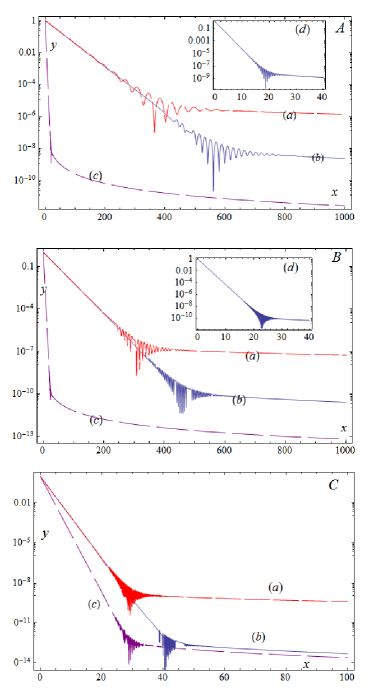
Figure 1: Axes: $x=t/\tau_{0}$ — time is measured in lifetimes $\tau_{0}$; $y$ — survival probabilities (the logarithmic scale). In all panels: $(a)$ the survival probability ${\cal P}_{p}(t)$, $(b)$ the survival probability ${\cal P}_{0}(t/\gamma_{L})$, $(c)$ the survival probability ${\cal P}_{0}(t)$ and $(d)$ is the enlarged part of $(c)$ showing the form of the decay curve ${\cal P}_{0}(t)$ for times $t\sim T_{0}$ belonging to the transition times region. Panel $A$: $\gamma_{L}\simeq 30.0167$ which corresponds to $m_{0}/{\it\Gamma}_{0}=10$ and $p/{\it\Gamma}_{0}=300$; panel $B$: $\gamma_{L}\simeq 20.025$, ($m_{0}/{\it\Gamma}_{0}=25$ and $p/{\it\Gamma}_{0}=500$); panel $C$: $\gamma_{L}=\sqrt{2}$ which corresponds to $m_{0}/{\it\Gamma}_{0}=100$ and $p/{\it\Gamma}_{0}=100$.

Results presented in these Figures enable us to compare decay curves of a moving relativistic unstable particle obtained within a correct relativistic treatment of the evolving in time $t$ and moving particle having certain momentum $p$ seen by an observer $\cal O$ in his rest system with those followed from the standard classical reasoning that in order to obtain relativistic effects for such a particle it is sufficient to replace $t$ by $t^{\prime}=t/\gamma_{L}$ (see (1)). Note that these results are in perfect agreement with analytical estimations (19), (23) and (24) performed for the model considered.

A similar comparison can be done in the case of the instantaneous energy ${\cal E}^{p}(t)$ of the moving unstable particle, which was discussed in [16] where it was shown that fluctuations of this energy are responsible for a possible emission of the electromagnetic radiation by moving charged unstable particles. Changes of these energies relative to the energy of the moving particle at the canonical decays time region (where the survival probability has the exponential form), $E_{0}(p)=\sqrt{p^{2}+m_{0}^{2}}$, are presented in Fig 2 in the form of ratios: $\kappa_{p}(t)\stackrel{{\scriptstyle\rm def}}{{=}}\frac{{\cal E}^{p}(t)-{\cal E}^{p}_{as}}{E_{0}(p)-{\cal E}^{p}_{as}}$, (here ${\cal E}^{p}_{as}=p$ — see (27)), and $\kappa_{0}(t)=\frac{{\cal E}^{0}(t)-{\cal E}^{0}_{as}}{E_{0}-{\cal E}^{0}_{as}}$, (here: $E_{0}={E_{0}(p)\,\vline}_{\,p=0}\equiv m_{0}$, ${\cal E}^{0}_{as}=\;E_{min}\equiv\mu_{0}=0$ and ${\cal E}^{0}(t)=\Re\,[h^{0}(t)]$, $h^{0}(t)={h^{p}(t)\vline}_{\,p=0}$).

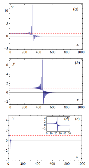
Figure 2: Axes: $x=t/\tau_{0}$, and $y$ — instantaneous energies: panel $(a)$ $\kappa_{p}(t)$; panel $(b)$ $\kappa_{0}(t/\gamma_{L})$ and panel (c) $\kappa_{0}(t)$. The horizontal dashed line denotes the values of $\kappa$-s equal to $1$. Here $\gamma_{L}=20.025$ which corresponds to $m_{0}/{\it\Gamma}_{0}=25$ and $p/{\it\Gamma}_{0}=500$.

4 Discussion and final remarks

Reasonable and physically acceptable models of unstable particles defined by means of the density $\omega(m)$ usually have the following form: $\omega(m)=\omega_{BW}(m)\;\times\;(m-\mu_{0})^{\lambda}\,\times\,f(m)$, where $\lambda\geq 0$ and $f(m)$ is a form–factor — it is a smooth function going to zero as $m\rightarrow\infty$ and it has no threshold and no pole. It appears that a behavior of the amplitudes, $a_{0}(t)$, defined by such a density $\omega(m)$ and by $\omega_{BW}(m)$ as functions of time $t$ is very similar (see [22, 5]). So conclusions following from the results obtained in Sec. 3 and 4 seems to be sufficiently general.

Results presented in Sec. 3 and 4 show that the relation (1) can be considered as a sufficiently accurate only for no more than a few lifetimes $\tau_{0}$ and that the supposition that (1) holds for times $t\gg\tau_{0}$ is wrong. It is because the assumption that ${\cal P}_{p}(t)\stackrel{{\scriptstyle\bf?}}{{=}}{\cal P}_{0}(t/\gamma_{L})$ is the classical physics relation. An extension of it to quantum decay processes does not lead to a significant error only for times $t$ when classical and quantum decay laws have a similar classical form, that is the exponential form. When quantum effects force the survival probability ${\cal P}_{p}(t)$ to behave nonclassically then the relation (1) is wrong and it may lead to the incorrect interpretation of decays of relativistic particles. Such a possible hypothetical situation is presented in Fig. 3: The temporal behavior of the real decay process of a relativistic particle at time intervals containing times $t$ significantly smaller than $T_{p}$ is described by the survival probability ${\cal P}_{p}(t)$ and it is shown by the solid line in this Figure, whereas the dashed line represents ${\cal P}_{0}(t/\gamma_{L})$ and according to (1) it is usually interpreted as the correct illustration of the decay process of such a particle.

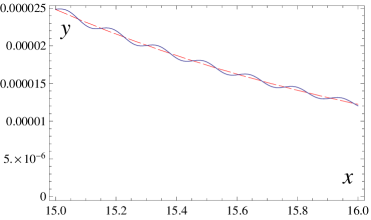
Figure 3: The case $m_{0}/{\it\Gamma}_{0}=100$ and $p/{\it\Gamma}_{0}=100$ (which gives $\gamma_{L}=\sqrt{2}$): The enlarged part of the decay curves $(a)$ and $(b)$ in Panel $(C)$ of Fig. 1. Axes: $x=t/\tau_{0}$, and $y$ — survival probabilities: Solid line — the survival probability ${\cal P}_{p}(t)$; Dashed line — the survival probability ${\cal P}_{0}(t/\gamma_{L})$.

In Fig. 1 are compared decay curves, that is survival probabilities ${\cal P}_{p}(t)$, obtained within the correct relativistic treatment of evolving in time and moving unstable particles with a given momentum $p$ relative to the rest system of the observer $\cal O$ as seen by this observer, with those obtained assuming the validity of the standard classical reasoning that in order to get decay curves of such particles it is sufficient to replace time $t$ in ${\cal P}_{0}(t)$ obtained using (5) by $t^{\prime}=t/\gamma_{L}$, that is it is enough to consider ${\cal P}_{0}(t/\gamma_{L})$ instead of ${\cal P}_{0}(t)$. Numerical results presented in this Figure are entirely consistent with the analytical results obtained in Sec. 2.

From (12), (23) and (24), or comparing decay curves $(a)$ and $(b)$ in Fig. 1, one can conclude that in the case of moving particles the transition time regions begin much more earlier than one could expect using the relation (1). For some combinations of $m_{0}/{\it\Gamma}_{0}$ and $p/{\it\Gamma}_{0}$ the transition times regions can begin even earlier in the case of moving particles, $p\neq 0$, than such a time region in the case of the particle observed in its rest system, $p=0$, (see Fig. 1, Panel $C$. A consequence of this fact is that ${\cal P}_{p}(T_{p})\gg{\cal P}_{0}(T_{0}/\gamma_{L})$ for times $t\geq T_{p}$. What is more, from results obtained in Sec. 2 and 3 it is seen that correctly obtained survival probability ${\cal P}_{p}(t)$ tends to zero as $t\rightarrow\infty$ much more slowly than ${\cal P}_{0}(t/\gamma_{L})$: Within the model considered ${\cal P}_{p}(t)\sim 1/t$ and ${\cal P}_{0}(t/\gamma_{L})\sim 1/t^{2}$ for $t\rightarrow\infty$ which confirms the conclusions presented in [20]. So if the initial number of unstable particles was ${\cal N}_{0}$, then the real number of moving unstable particles ${\cal N}(T_{p})$ which had a chance to survive up to time $t\sim T_{p}$ or later and which were registered by the observer $\cal O$ is much greater than the corresponding number ${\cal N}(T_{0}/\gamma_{L})$ obtained assuming the validity of (1): There is ${\cal N}(T_{p})={\cal P}_{p}(T_{p})\,{\cal N}_{0}\,\gg\,{\cal N}(T_{0}/\gamma_{L})={\cal P}_{0}(T_{0}/\gamma_{L})\,{\cal N}_{0}$. A similar conclusion holds for times $t>T_{p}$. This effect may be important when interpreting results of some accelerator experiments with high energy unstable particles and also when interpreting some results of astrophysical observations. Astrophysical processes are the source of a huge number of elementary particles including unstable particles of very high energies. The numbers of created unstable particles during these processes are so large that many of them may survive up to transition times $t\sim T_{p}$ or much later and they move with ultra relativistic velocities. From the above discussion it follows that numbers of unstable particles which survived to these times is much, much greater than one could expect estimating these numbers by means of the relation (1).

The above analysis shows also that the scale and the intensity of the effect described in [16] were underestimated there. In [16] the instantaneous energy ${\cal E}_{\phi}(t)$ of an unstable particle $\phi$ was analyzed and it was shown there that fluctuations of this energy at the transition time region have to occur. These fluctuations cause changes in the particle velocity which in the case of charged particles (or particles with the non–zero magnetic moment) forces them to emit electromagnetic radiation. The base of estimations performed in [16] was the relation of the type (1). Results presented in Fig. 2 show that in the case of the moving relativistic particle the form of these fluctuations seen by the observer ${\cal O}$ is the same as the form o such fluctuations in the particle rest system but they occur much earlier. What is more the amplitude of fluctuations of ${\cal E}_{\phi}^{p}(t)$ may be even larger than the corresponding amplitude of ${\cal E}_{\phi}(t)$ calculated in the particle rest system. Also the analysis performed in this Section and results presented in Fig. 1 shows that in a real situation much more unstable particles have to survive up to the transition times than it can be expected using (1) when performing the estimations. In general one can expect that within the model considered the relation between true number of the particles, ${\cal N}(t\sim T_{p})={\cal P}_{p}(t\sim T_{p})\,{\cal N}_{0}$, which survived up to $t\sim T_{p}$, and the corresponding number ${\cal N}(t\sim T_{0}/\gamma_{L})$ obtained assuming (1) looks as follows: ${\cal N}(t\sim T_{p})\,\gtrsim\,10^{3}\,{\cal N}(t\sim T_{0})$ (compare curves $(a)$ and $(b)$ analyzed in these Figures for times $t$ belonging to the transition times region and values of the corresponding survival probabilities). This means that the scale of effect analyzed in [16] and its intensity should be much larger than it was estimated there.

The last remarks. There is a remarkable similarity of decay curves presented in Fig. 3 and results reported by the GSI team in [27] and presented there in Figs 3 and 5 (for update results see [28]). The relativistic Lorentz factor in the GSI experiment was $\gamma_{L}\simeq 1.43$ which is very close to the Lorentz factor used in calculations leading to the results presented in our Fig. 1, Panel $C$, and Fig. 3. In Fig. 3 the solid fluctuating decay curve ${\cal P}_{p}(t)$ looks as the curve obtained experimentally by the mentioned GSI team, whereas the dashed curve being a part of exponentially decreasing probability ${\cal P}_{0}(t/\gamma_{L})$ at these times $t$ looks as the expected and calculated theoretically curve by this team. So one can not exclude that choosing an appropriate form of the density $\omega(m)$ rather different from the simple $\omega_{BW}(m)$ (e.g. having the form discussed in [29]) and calculating the survival probability ${\cal P}_{p}(t)$ by means of the proper formula (18) it will be possible to reproduce theoretically the experimental decay curve obtained by the GSI team and thus to explain the GSI anomaly.

Acknowledgments: This work was supported in part by the Polish NCN project DEC–2013/09/B/ST2/03455.

References

- [1] B. Misra and E. C. G. Sudarshan, J. Math. Phys. 18, 756 (1977).
- [2] C. B. Chiu, B. Misra, and E. C. G. Sudarshan, Phys. Rev. D 16, 520 (1977);
- [3] W. C. Schieve, L. P. Horwitz, and J. Levitan, Phys. Lett. A 136, 264 (1989); A. G. Kofman and G. Kurizki, Nature 405, 546 (2000).
- [4] L. A. Khalfin, Zh. Eksp. Teor. Fiz. 33, 1371 (1957) [Sov. Phys. — JETP 6, (1958), 1053].
- [5] L. Fonda, G. C. Ghirardii and A. Rimini, Rep. on Prog. in Phys. 41, 587 (1978).
- [6] J. M. Wessner, D. K. Andreson and R. T. Robiscoe, Phys. Rev. Lett. 29, (1972), 1126.
- [7] E. B. Norman, S. B. Gazes, S. C. Crane and D. A. Bennet, Phys. Rev. Lett. bf 60, (1988), 2246. E. B. Norman, B. Sur, K. T. Lesko, R.-M. Larimer, Phys. Lett. B 357, (1995), 521.
- [8] J. Seke, W. N. Herfort, Phys. Rev. A 38, (1988), 833.
- [9] R. E. Parrot, J. Lawrence, Europhys. Lett. 57, (2002), 632.
- [10] J. Lawrence, Journ. Opt. B: Quant. Semiclass. Opt. 4, (2002), S446.
- [11] I. Joichi, Sh. Matsumoto, M. Yoshimura, Phys. Rev. D 58, (1998), 045004.
- [12] N. G. Kelkar, M. Nowakowski and K. P. Khemchandani, Phys. Rev. C 70, (2004), 024601.
- [13] M. Nowakowski, N. G. Kelkar, arXiv: 0807.5103; AIP Conf. Proc. 1030, (2008), 250.
- [14] T. Jiitoh, S. Matsumoto, J. Sato, Y. Sato, K. Takeda, Phys Rev. A 71, (2005), 012109.
- [15] C. Rothe, S. I. Hintschich and A. P. Monkman, Phys. Rev. Lett. 96, 163601 (2006).
- [16] K. Urbanowski, K. Raczyńska, Phys. Letters B731, 236 (2014).
- [17] P. Exner, Phys. Rev. D 28, 2611 (1983).
- [18] L. A. Khalfin, Quantum theory of unstable particles and relativity, PDMI PREPRINT–6/1997 (St. Petersburg Department of Steklov Mathematical Institute, St. Pteresburg, Russia, 1997).
- [19] E. V. Stefanovitch, Quantum effects in relativistic decays, International Journal of Theoretical Physics, 35, 2539 (1996).
- [20] M. Shirkov, Decay law of a moving unstable particles, International Journal of Theoretical Physics, 43, 1541 (2004).
- [21] S. Krylov, V. A. Fock, Zh. Eksp. Teor. Fiz. 17, (1947), 93.
- [22] N. G. Kelkar, M. Nowakowski, J. Phys. A: Math. Theor., 43, 385308 (2010).
- [23] K. Urbanowski, Eur. Phys. J. C 58, 151, (2008).
- [24] W. M. Gibson, B. R. Polard, Symmetry principles in elementary particle physics, Cambridge, 1976.
- [25] K. Urbanowski, Eur. Phys. J. D 54, 25 (2009).
- [26] K. Urbanowski, Phys. Rev. A 50, 2847 (1994).
- [27] Yu.A. Litvinov et al, Physics Letters B 664, 162 (2008).
- [28] P. Kienle et al, Physics Letters, B 726, 638 (2013).
- [29] F. Giacosa, G. Pagliara, Quantum Matter, 2, 54, (2013); arXiv: 1110.1669. F. Giacosa, G. Pagliara, (Oscillating) non–exponetial decays of unstable states, arXiv: 1204.1896.