The Fast Multipole Method and Point Dipole Moment Polarizable Force Fields

Abstract

We present an implementation of the fast multipole method for computing coulombic electrostatic and polarization forces from polarizable force-fields based on induced point dipole moments. We demonstrate the expected $O(N)$ scaling of that approach by performing single energy point calculations on hexamer protein subunits of the mature HIV-1 capsid. We also show the long time energy conservation in molecular dynamics at the nanosecond scale by performing simulations of a protein complex embedded in a coarse-grained solvent using a standard integrator and a multiple time step integrator. Our tests show the applicability of FMM combined with state-of-the-art chemical models in molecular dynamical systems.

I Introduction

In $N$-body simulations, the long-range potentials, such as gravitational or electrostatic potentials, pose the greatest computational difficulty as their cost scales with the number of particles as $O(N^{2})$. Reducing this complexity has been the subject of intense study for over 40 years and has seen the development of many successful algorithms. Particularly important have been the Ewald summation scheme, which achieved a scaling of $O(N^{3/2})$ (Perram, Petersen, and De Leeuw, 1988), and its extension, the particle-mesh-Ewald (PME) scheme (Darden, York, and Pedersen, 1993) based on fast Fourier transforms (FFTs), which scales as $O(N\log N)$. The tree-code from Barnes and Hut (1986) also reduced the cost to $O(N\log N)$ using multipole expansions of the potential. From a purely algorithmic perspective, the most performant algorithm should be the fast multipole method (FMM) proposed by Greengard and Rokhlin (1987), which scales as $O(N)$. However, despite volumes of theoretical work, the FMM, on which we focus here, has not been widely used in production molecular dynamics (MD) simulations due to the perceived complexity to implement it, hidden constants that affect its scaling, issues with multiple time step integrators, and early concerns that energy cannot be conserved well enough unless a prohibitively high accuracy is used (Bishop, Skeel, and Schulten, 1997; Figueirido et al., 1997). For these reasons, PME is presently very popular among many molecular dynamics codes (Sagui and Darden, 1999) to handle periodic molecular systems containing up to millions of atoms (Zhao et al., 2013), even if FFT does not scale well on modern supercomputer architectures due to high communication overhead.

Interest in FMM has recently resurfaced again because of these scaling problems and the desire to solve much larger systems (Arnold et al., 2013; Yokota and Barba, 2012). Several successful implementations have existed in the astrophysics community for many years to evolve the extremely large number of particles typically representing dark matter (e.g., Diemand et al., 2008; Stadel et al., 2009). In this paper we present an implementation of FMM to perform molecular dynamics simulations based on advanced many-body interatomic potentials (force-fields) including polarization effects described according to the induced point dipole approach.

The development of polarizable force-fields represents an important step in molecular modeling, as such fields have been shown to greatly improve the description of complex microscopic systems, such as physical interfaces and those involving charged species (Dang, 2000; Lopes, Roux, and MacKerell Jr, 2009; Cieplak et al., 2009; Chang and Dang, 2006; Jungwirth and Tobias, 2006; Réal et al., 2013; Salanne and Madden, 2011). Polarization is also suspected to greatly improve the description of amino-acid interactions, which will lead to further promising computational techniques devoted to theoretically investigations of protein folding (Scarpazza et al., 2013).

Among the polarizable force-fields proposed so far, the second author has developed a particular kind of force-field which couples easily and efficiently with a polarizable coarse grained approach to model the solvent (Masella, Borgis, and Cuniasse, 2008, 2011). Here, a complex solute (e.g., a protein) is modelled at the atomic level while the solvent is modeled as a set of polarizable pseudo-particles. The main feature of this approach is the systematic cut off of the solute-solvent interactions whose computation scales as $O(N)$ (with $N$ the atomic solute size), while no cut off is considered in computing intra-solute interactions. In other words, the computation of intra-solute electrostatic interactions corresponds to an electrostatic free boundary condition problem. Hence, coupling the modeling approach and an FMM scheme to compute the intra-solute interactions will lead to a full $O(N)$ polarizable approach to investigate the solvation of large and complex solutes, without applying any cut-off to intra-solute interactions. Note that even if the solute-solvent interactions are truncated for distances larger than a reference one (typically 12 Å), we recently proposed a multi-scale, coarse grained approach, which allows the solute-solvent truncation drawbacks to be minimized, while still maintaining the $O(N)$ complexity of the solute-solvent interaction computational scheme (Masella, Borgis, and Cuniasse, 2013a).

Our FMM method is based on the work of Dehnen (2002) that uses a binary tree spatial decomposition and conserves linear momentum by construction (via a dual tree walk approach to compute multipole interactions). Accuracy is controlled by an opening angle tolerance parameter $\theta$ at fixed multipole expansion order.

In this paper we first review in §II the induced point dipole method and the mathematical basis of FMM. In §III we discuss some technical details of our implementation and in §IV we present tests of the accuracy and precision, particularly when coupling FMM with a multiple time steps integrator devoted to induced dipole moment based force-fields. We also discuss the efficiency of an FMM approach compared to PME when simulating a large molecular system and accounting for polarization. We present our conclusions in §V.

II Theory

II.1 Induced point dipole polarizable force-fields

Molecular modeling approaches consider the total interatomic potential $U$ as a sum of different energy terms. For polarizable force-fields, a sum of four terms is commonly considered

$$U=U^{\mathrm{short}}+U^{\mathrm{rel}}+U^{qq^{\prime}}+U^{\mathrm{pol}}$$ (1)

Here, $U^{\mathrm{short}}$ is a short range energy term describing the short range atom-atom repulsive effects and, usually, dispersion effects. The term is normally additive in nature, however, there have been attempts to consider short range many-body potentials to account for short range electronic cloud reorganization effects (e.g., Réal et al., 2013). $U^{\mathrm{rel}}$ is the sum of the common stretching, bending and torsional potentials, which describe the interactions among covalently bonded atoms.

The standard pairwise Coulomb potential $U^{qq^{\prime}}$ is based on static charges centered on the system atoms

$$U^{qq^{\prime}}=\frac{1}{2}\sum_{i}\Phi^{q}_{i}=\dfrac{1}{8\pi\epsilon_{0}}\sum_{i}q_{i}\sum^{*}_{j}{q_{j}\phi(\bm{x}_{i}-\bm{x}_{j})}$$ (2)

where the Green’s function is $\phi(\bm{x}_{i}-\bm{x}_{j})={|\bm{x}_{i}-\bm{x}_{j}|^{-1}}$. The superscript ^∗ denotes sums for which a subset of atoms is excluded (commonly, the atoms $j$ separated by less than two chemical bonds from an atom $i$).

$U^{\mathrm{pol}}$ is the polarization term. When considering an induced dipole moment polarization approach, a set of additional degrees of freedom is introduced, the induced dipole moments $\bm{\mu}_{i}$, that obey

$$\bm{\mu}_{i}=\bm{\mathsf{\alpha}}_{i}\cdot\left(\bm{E}_{i}^{q}+\bm{E}^{\mu}_{i}\right)$$ (3)

Here, $\bm{\mathsf{\alpha}}_{i}$ is the polarizability tensor of the polarizable atom $i$, $\bm{E}_{i}^{q}$ and $\bm{E}^{\mu}_{i}$ are the electric fields generated on atom $i$ by the surrounding static charges $q_{j}$ and the surrounding induced dipoles $\bm{\mu}_{j}$, respectively. These two electric fields are defined as

$$\bm{E}^{q}_{i}=-\sum_{j}^{*}q_{j}\ \bm{\nabla}\phi(\bm{x}_{i}-\bm{x}_{j})$$ (4)

and

$$\bm{E}^{\mu}_{i}=-\sum_{j}^{*}\bm{\mu}_{j}\cdot\bm{\mathsf{T}}_{ij}$$ (5)

The dipolar tensor $\bm{\mathsf{T}}_{ij}$ is the second derivative of the Green’s function

$$\bm{\mathsf{T}}_{ij}=\bm{\nabla}^{2}\phi(\bm{r}=\bm{x}_{i}-\bm{x}_{j})=\frac{1}{r^{3}}\left({\bm{\mathsf{1}}}-{{3\bm{r}\otimes\bm{r}}\over{r^{2}}}\right)$$ (6)

where $\otimes$ is the tensor outer product. $\bm{\mathsf{T}}_{ij}$ is, however, usually altered to account for interatomic short range damping effects. Following the original ideas of Thole (1981), this is achieved by adding to $\bm{\mathsf{T}}_{ij}$ a specific short range dipolar tensor $\bm{\mathsf{T}}_{ij}^{\mathrm{damp}}$.

The interactions of the dipoles with the above two electric fields give rise to two additional potentials, namely

$$\Phi^{\mu q}_{i}=\bm{\mu}_{i}\cdot\bm{E}^{q}_{i}\quad\mathrm{and}\quad\Phi^{\mu\mu}_{i}=\bm{\mu}_{i}\cdot\bm{E}^{\mu}_{i}$$ (7)

$U^{\mathrm{pol}}$ also typically accounts for a third energy term, $A(\bm{\mu})$, quantifying the energy cost to create a dipole $\bm{\mu}$. In standard induced dipole moment implementations, this third term leads to the fundamental relationship

$${\partial U^{\mathrm{pol}}\over\partial\bm{\mu}}=0$$ (8)

For instance, when the dipoles obey the linear relation (3) and the polarizability tensors $\bm{\mathsf{\alpha}}_{i}$ are taken as isotopic polarizabilities (i.e., they are a scalar quantity), the above condition is met by taking

$$A(\bm{\mu})=\frac{1}{2}\sum_{i}{\ |\bm{\mu}_{i}|^{2}\over\bm{\alpha}_{i}}$$ (9)

Note that alternative induced dipole moment approaches where the dipoles obey more complex relations have been proposed (e.g., Ha-Duong et al., 2002). In that case, a specific $A(\bm{\mu})$ energy term is considered that fulfills the relation (8). Regardless of the form of $A(\bm{\mu})$, the total dipole potential energy nevertheless obeys

$$U^{\mathrm{pol}}=A(\bm{\mu})-\sum_{i}\Phi^{\mu q}_{i}-\frac{1}{2}\sum_{i}\Phi^{\mu\mu}_{i}$$ (10)

II.2 The Fast Multipole Method

The fast multipole method (FMM) (Greengard and Rokhlin, 1987) is a technique for approximating a long range potential

$$\Phi(\bm{x}_{b})=\sum_{a\in\bm{\mathcal{P}}}q_{a}\phi(\bm{x}_{b}-\bm{x}_{a})$$ (11)

of a set of particles $\bm{\mathcal{P}}$ via a multipole expansion of the Green’s function $\phi$. Typically, the particles are organized by a hierarchical spatial decomposition such as an oct-tree or binary tree. We consider the interaction of the multipole expansions of the particles in pairs of tree nodes $A,B$ centered at $\bm{z}_{A},\bm{z}_{B}$, and containing particles labeled $a$ and $b$, respectively.

The Taylor expansion of $\phi$ to $p^{\mathrm{th}}$ order about both centers in Cartesian coordinates yields the following expression

$$\phi(\bm{x}_{b}-\bm{x}_{a})\approx\sum_{|\bm{\mathsf{n}}|\leq p}\sum_{|\bm{\mathsf{m}}|\leq p-|\bm{\mathsf{n}}|}\frac{(-1)^{|\bm{\mathsf{n}}|}}{\bm{\mathsf{n}}!\bm{\mathsf{m}}!}\bm{r}_{b}^{\bm{\mathsf{n}}}\bm{r}_{a}^{\bm{\mathsf{m}}}\bm{\nabla}^{\bm{\mathsf{n}}+\bm{\mathsf{m}}}\phi(\bm{z}_{B}-\bm{z}_{A})$$ (12)

where $\bm{r}_{b}=\bm{x}_{b}-\bm{z}_{B}$ and $\bm{r}_{a}=\bm{x}_{a}-\bm{z}_{A}$. Here we make use of multi-index notation, whose relevant properties are summarized in §D.

Grouping terms, we can express the multipole expansion for a node $A$ (or $B$) as

$$M_{\bm{\mathsf{n}}}(\bm{z}_{A})=\sum_{a\in A}q_{a}\frac{(-1)^{|\bm{\mathsf{n}}|}}{\bm{\mathsf{n}}!}\bm{r}_{a}^{\bm{\mathsf{n}}}$$ (13)

Multipoles can be computed efficiently for all parent nodes by combining the multipoles of child nodes using the shifting operator

$$M_{\bm{\mathsf{n}}}(\bm{z}+\bm{x})=\sum_{|\bm{\mathsf{k}}|\leq|\bm{\mathsf{n}}|}\frac{\bm{x}^{\bm{\mathsf{k}}}}{\bm{\mathsf{k}}!}M_{\bm{\mathsf{n}}-\bm{\mathsf{k}}}(\bm{z})$$ (14)

If two nodes are sufficiently distant for the expansions to be accurate—as determined by an implementation specific multipole acceptance criteria (MAC) which we will discuss later—the multipoles may be transformed into a local expansion (or field tensor) about another point, e.g.,

$$F_{\bm{\mathsf{n}}}(\bm{z}_{B})=\sum_{|\bm{\mathsf{m}}|\leq p-|\bm{\mathsf{n}}|}M_{\bm{\mathsf{m}}}(\bm{z}_{A})\bm{\nabla}^{\bm{\mathsf{n}}+\bm{\mathsf{m}}}\phi(\bm{z}_{B}-\bm{z}_{A})$$ (15)

Performing this evaluation on both $A$ and $B$ symmetrically naturally satisfies Newton’s third law.

The final evaluation of the potential proceeds as follows. The field tensors from node-node interactions are accumulated from parent to child down the tree by the shifting formula

$$F_{\bm{\mathsf{n}}}(\bm{z}+\bm{x})=\sum_{|\bm{\mathsf{k}}|\leq p-|\bm{\mathsf{n}}|}\frac{\bm{x}^{\bm{\mathsf{k}}}}{\bm{\mathsf{k}}!}F_{\bm{\mathsf{n}}+\bm{\mathsf{k}}}(\bm{z})$$ (16)

such that $F_{\bm{\mathsf{n}}}$ in the leaf nodes will be the sum of all the field tensors of all parent nodes and any node-node interactions it had itself. The approximated potential (or any $k^{\mathrm{th}}$ order derivative) at the positions of particles in a leaf node $B$ is then

$$\bm{\nabla}^{k}\Phi(\bm{x}_{b})\approx q_{b}\sum_{|\bm{\mathsf{n}}|\leq p-k}\frac{1}{\bm{\mathsf{n}}!}(\bm{x}_{b}-\bm{z}_{B})^{\bm{\mathsf{n}}}F_{\bm{\mathsf{n}}+k}(\bm{z}_{B})$$ (17)

II.3 FMM and induced point dipole moments

An induced point dipole $\bm{\mu}_{i}$ can be viewed as resulting from a pair of particles with charges $\pm q^{\mu}_{i}$ located at a distance $|\delta\bm{l}_{i}|$ from the dipole center such that

$$\bm{\mu}_{i}=2|q^{\mu}_{i}|\delta\bm{l}_{i}$$ (18)

From the above relation, it is straightforward to compute the polarization energy and forces using FMM. With the dipole charge set $\{q^{\mu}_{i}\}$ and by considering $\bm{x}_{i}^{\pm}=\bm{x}_{i}\pm\delta\bm{l}_{i}$, we can reformulate the potentials in $U^{\mathrm{pol}}$ such that they take a similar form as the standard Coulomb potential

$$\Phi^{\mu q}_{i} =\bm{\mu}_{i}\cdot\bm{E}^{q}_{i}$$

$$=q^{\mu}_{i}\sum_{j}^{*}q_{j}\left(\phi(\bm{x}_{i}^{+}-\bm{x}_{j})-\phi(\bm{x}_{i}^{-}-\bm{x}_{j})\right)$$ (19)

and

$$\Phi^{\mu\mu}_{i} =\bm{\mu}_{i}\cdot\bm{E}^{\mu}_{i}$$

$$=q^{\mu}_{i}\sum_{j}^{*}q^{\mu}_{j}\left[\left(\phi(\bm{x}_{i}^{+}-\bm{x}_{j}^{+})-\phi(\bm{x}_{i}^{+}-\bm{x}_{j}^{-})\right)\right.$$

$$\qquad\qquad\;\;\left.-\left(\phi(\bm{x}_{i}^{-}-\bm{x}_{j}^{+})-\phi(\bm{x}_{i}^{-}-\bm{x}_{j}^{-})\right)\right]$$ (20)

Note that if $U^{\mathrm{pol}}$ obeys Eq. (8), then the derivatives of $U^{\mathrm{pol}}$ with respect to the charges $\{q^{\mu}_{i}\}$ and the vectors $\delta\bm{l}_{i}$ vanish. Hence, all the formulas discussed in the above section can be used as such to compute the polarization energy and forces. The same $p^{\mathrm{th}}$ order expansion is used to estimate equations (19) and (20) as for the Coulomb potential despite $\bm{\mu}_{i}$ being related to a second order derivative of the Green’s function. Our later tests suggest this has no effect on the resulting precision of the simulations.

Moreover, the electric fields in equation (3), which the induced dipole moments obey, are also computable using FMM. The static electric field $\bm{E}_{i}^{q}$ can be computed by considering the spatial derivatives of the electrostatic potential acting on atom $i$ and generated by the surrounding charges $q_{j}$. Likewise, the dynamical electric field $\bm{E}_{i}^{\mu}$ can be computed by considering the spatial derivatives of the electrostatic potential generated on atom $i$ by the surrounding set of charges $q^{\mu}_{j}$.

III Implementation

Here we will describe briefly our implementation of the FMM in our own molecular dynamics code Polaris(MD) (Masella, Borgis, and Cuniasse, 2008, 2011, 2013b). The implementation is similar to that described in Dehnen (2002), but we account for the Coulomb, dipole-static electric field, and dipole-dipole interactions. Moreover, we also account for the specificities of the polarizable force-fields implemented in the code Polaris(MD) by allowing only a subset of atoms to generate the static electric field acting on a second subset of polarizable atoms (both these subsets of atoms can be different, and the charges $q^{E}_{i}$ generating the electric field can also be different from the Coulomb $q_{i}$ ones (Masella and Cuniasse, 2003)). The atomic polarizability tensor $\bm{\mathsf{\alpha}}_{i}$ is taken to be isotropic and is replaced by a scalar $\alpha_{i}$.

Regardless of the charge set generating a potential, the approximate potential $\Phi$ consists of two components

$$\Phi=\Phi^{\mathrm{direct}}+\Phi^{\mathrm{fmm}}$$ (21)

The first component is computed via direct particle-particle interactions while the second is computed via FMM. The direct component includes particles that are too close for the multipole expansion to be accurate enough and also for interactions that are cheaper to compute directly than with the expansions. Other effects, such as damping the polarization effects at short range and the atom-atom repulsive potential $U^{\mathrm{rep}}$ are also computed directly using a list of neighbors when a cell has a “self”-interaction. We explicitly consider the induced dipole moments {$\bm{\mathsf{\mu}}_{i}$} for direct particle-particle interactions and not the $q^{\mu}_{i}$ and $\delta\bm{l}_{i}$ quantities.

The atoms are organized via an adaptive kd-tree spatial decomposition. A binary tree, as opposed to an oct-tree, is particularly well suited for non-uniformly distributed structures, or structures that are not roughly cubic in extent. This is an important feature for simulating a complex solute solvated within a coarse-grained solvent box (see below). For efficiency, we build one tree with all the atoms $\mathcal{T}^{\mathrm{atom}}$ and a second tree with only the polarizable atoms $\mathcal{T}^{\mu}$.

The tree is constructed by recursively splitting the bounding volume across the longest dimension at the location of the geometric center of the particles within each cell. The recursion stops once a cell has no more than $N_{\mathrm{bucket}}$ particles, where $N_{\mathrm{bucket}}$ is a parameter we set to 8. Larger values decrease the size of the tree at the expense of increased direct sum work. The multipole expansions are computed for all leaf nodes and then combined up the tree to the root node. For cells with dipole sites, the two-particle approximation discussed in §II.3 is computed on the fly and the contribution of the two particles is added to the multipole. The two particles are never considered as real particles in the simulation and are not part of the domain decomposition. This avoids a potential problem whereby a cell boundary might divide a dipole pair.

In addition to typical tree book keeping data, each cell stores information for each of the three categories of particles: all atoms, atoms generating $\bm{E}^{q}$, and polarizable atoms. This information includes the geometric center $\bm{z}$ of the particle positions; the bounds of the tightest enclosing box $\bm{x}_{\mathrm{min}},\bm{x}_{\mathrm{max}}$; the distance $r_{\mathrm{enc}}$ from $\bm{z}$ to the most distant corner of the bounding box; the multipole coefficients $M_{\bm{\mathsf{n}}}$; and the field tensor coefficients $F_{\bm{\mathsf{n}}}$. For cells with less than 3 particles, we add a small padding to avoid planar or singular box sizes. The choice of radius $r_{\mathrm{enc}}$ allows parent cell sizes and positions to be easily derived from the children. Each cell requires approximately $N_{\mathrm{cellsize}}=3200$ bytes. Hence, assuming a perfectly balanced tree, a simulation with $N=10^{6}$ particles would currently only require $2N/N_{\mathrm{bucket}}\times N_{\mathrm{cellsize}}\sim 810$ MB to store the tree.

We control the accuracy of the multipole calculation by fixing the expansion order $p$ of the multipoles and defining the user adjustable parameter $\theta\in[0,1)$. Nodes $A,B$ are allowed to interact via their multipoles if they satisfy the multipole acceptance criteria (MAC)

$$\theta\cdot|\bm{z}_{A}-\bm{z}_{B}|>(r_{\mathrm{enc},A}+r_{\mathrm{enc},B})$$ (22)

When $\theta=1$ the enclosing spheres of the nodes are allowed to be exactly touching, while when $\theta=0$ the nodes are never allowed to interact via their multipoles and all interactions are computed using a direct sum. The FMM of Greengard and Rokhlin (1987) controls accuracy in a similar manner with the expansion order $p$ of the multipoles and a well-separated parameter $ws$ that determines the minimum distance for a multipole interaction.

Very recent work by Dehnen (2014) suggests that at $\theta=1$ only small improvements to the precision are gained by large increases in $p$, while at $\theta<1$ large gains in precision are possible for small changes in $p$. In §IV we explore a range of $\theta$ values while fixing the expansion order at $p=5$.

Interactions are determined by descending the tree in a dual-walk fashion whereby we maintain a stack of interaction pairs. The walk begins by placing nodes $A,B$ equal to the root node on the stack. At each iteration of the walk, the top most nodes are removed. A direct interaction between the nodes is considered if the total number of particles is less than $\sim$64, or the nodes are both leaves. If a direct interaction is not performed but the nodes satisfy the MAC, a multipole interaction is computed. The field tensors are accumulated for the mutual interaction of the nodes, thus ensuring conservation of momentum. If the MAC is not satisfied, interactions with the children of the node with the larger $r_{\mathrm{enc}}$ are placed on the stack. If the larger node happens to be a leaf, then the children of the smaller node are taken instead. By way of example, if node $B$ was larger, the interactions $AB_{\mathrm{left}}$, $AB_{\mathrm{right}}$, and $B_{\mathrm{left}}B_{\mathrm{right}}$ are placed on the stack. When the two nodes are equal and a self interaction is not possible then all unique combinations child interactions are placed on the stack. The procedure ends when there is no more work left on the stack.

Calculating all the long range forces involves several applications of the above procedure applied in three stages. We first calculate the coulomb forces $\bm{\nabla}\Phi^{q}$ and static electric field $\bm{E}^{q}$ using $\mathcal{T}^{\mathrm{atom}}$. All particles with non-zero $q_{i}$ interact with each other, but only those with non-zero $q^{E}_{i}$ are allowed to contribute to the electric field. The electric field is only evaluated at the positions of polarizable particles (those with non-zero $\bm{\mu}_{i}$). Second, we iteratively solve for the dipoles $\bm{\mu}_{i}=\alpha_{i}\cdot\bm{E}_{i}$ using $\mathcal{T}^{\mu}$. At each iteration we recalculate the moments and perform an FMM interaction tree walk. The details of the iterative procedure have been described earlier in Masella, Borgis, and Cuniasse (2008). This has been shown to allow large time steps to be used to solve the Newtonian equations of motion in MD simulations (Wang and Skeel, 2005), as well as multiple time step MD integrator (Masella, 2006). Finally, with the converged solution for the dipoles, we update the moments for the dipoles stored in $\mathcal{T}^{\mathrm{atom}}$ and compute the dipole-dipole forces as well as the dipole-$q^{E}$ forces.

IV Tests

To assess the quality of our implementation, both in terms of precision and efficiency, we performed a number of accuracy and performance tests. We compare the force evaluations with those generated by the standard $O(N^{2})$ implementation, which we refer to as a “direct” summation. Tests computed using a direct sum and involving polarized atoms use point dipoles and not the dipole approximation from §II.3.

We measure the relative error in the forces $\bm{a}_{i}$ of each particle via the quantity

$$f^{\mathrm{err}}_{i}={{|\bm{a}^{\mathrm{fmm}}_{i}-\bm{a}^{\mathrm{dir}}_{i}|}\over{|\bm{a}^{\mathrm{dir}}_{i}|}}$$ (23)

We chose to compare the force rather than potential as the force is the directly integrated quantity and because the potential is smoother and thus less likely to reveal any computational issues. Where timings are reported, the calculations were performed on a single core Intel Core i7 1.7GHz CPU. We compiled Polaris(MD) with production-run settings using the Intel ifort 14.0.3 compiler with the -O3, -xHost, and -ipo options and SIMD vectorization enabled.

Most of the tests were performed by considering different kinds of molecular systems in vacuum. For instance, we test the scaling properties of our FMM implementation using non-hydrated subsets of the HIV-1 capsid system. However, we also performed a series of tests with a protein complex solvated in a coarse grained solvent box, according to the computational approach proposed by the second author (Masella, Borgis, and Cuniasse, 2008, 2011). In that approach, the solvent is modeled by polarizable pseudo-particles, and both the solvent-solvent and solute-solvent interactions are truncated for distances longer than 7 Å and 12 Å, respectively. The algorithmic complexity concerning the solute-solvent and solvent-solvent interactions therefore scales as $O(N_{p})$ and $O(N_{s})$, where $N_{p}$ and $N_{s}$ are the number of protein atoms and solvent pseudo-particles, respectively. Moreover, periodic boundary conditions are used to maintain the solvent density within the simulation box. They are applied only to the solvent pseudo-particles, whereas the solute doesn’t interact with its own periodic images (i.e., the computation of electrostatic solute-solute interactions corresponds to a free boundary condition problem). Hence, during our tests, FMM is used only to compute intra-solute interactions and, as only atoms are involved in long range forces, we will ignore the solvent pseudo-particles in the discussions. Note that, as already mentioned in §I, to rectify the solvent model deficiencies originating from long range solute-solvent force truncation, we recently proposed a multi-level coarse-grained $O(N_{p})$ approach allowing one to minimize the solute-solvent truncation drawbacks, particularly in the case of a solute presenting charged moieties (Masella, Borgis, and Cuniasse, 2013a). The solvated protein tests discussed here will demonstrate the numerical accuracy of a solute(FMM)/solvent(coarse-grained) approach, whose complexity is $O(N)$ and which accounts for all the microscopic forces present in the system, regardless of their range.

IV.1 Sphere Tests

We first tested the FMM force accuracy using a randomly generated sphere of atoms. The sphere was generated by uniformly sampling 4096 points inside a radius of 45 Å with a minimum interparticle separation of 2 Å. An equal number of $q=\pm e$ charges were chosen such that the sphere would be charge neutral. Each atom was also assigned a random $q^{E}=\pm e$ charge for the electric field, but again in equal number to ensure neutrality.

In Figure 1 we show the relative error of the force with respect to the direct evaluation. Polarization effects are disabled so that only the Coulombic forces are considered. Three opening angles $\theta=0.5,0.7,0.99$ were chosen from more accurate to less accurate. For $\theta=0.5$ about 80% of the atoms have errors less than $10^{-4}$ and all are less than $10^{-2}$, as seen in the cumulative histograms. On our test machine, we measured the average FMM computation time to be 0.23 s, 0.12 s, and 0.07 s for the three $\theta$ values, respectively. The direct summation required 0.06 s. For such small systems the overhead introduced with FMM dominates the computation.

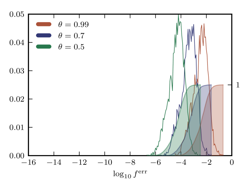
Figure 1: The relative FMM error of the force on each atom of the random sphere compared with a direct evaluation. Polarization is disabled. Three values of the tolerance parameter $\theta=0.5,0.7,0.99$ are considered, from very accurate to less accurate. The left vertical axis has been normalized such that the area under each curve is 1. Filled curves using the right vertical axis represent the cumulative histograms.

In Figure 2 we fix $\theta=0.5$, enable polarization, and recompute the forces. The polarization scalar for all atoms is taken to be $\alpha=\{0,1,2,3\}$, for each test, respectively. In the case of $\alpha=0$ the test is equivalent to that shown previously in Figure 1. In all cases there is no significant change in the error distribution.

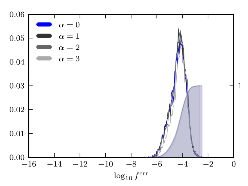
Figure 2: The relative FMM error of the force on each atom of the random sphere compared with a direct evaluation. Polarization is enabled with where the polarization scalar $\alpha\in{0,1,2,3}$ has been assumed for all atoms. The tolerance parameter is fixed at $\theta=0.5$. We highlight in blue the $(\alpha,\theta)=(0,0.5)$ case presented in Figure 1. The left vertical axis has been normalized such that the area under each curve is 1. Filled curves using the right vertical axis represent the cumulative histograms.

We also considered the effect of our choice of $|\delta\bm{l}|$, the separation distance for the point dipole approximation. Even though we tested values over 5 orders of magnitude, from $10^{-5}$ to $10^{-1}$ Å, as shown in Figure 3, we again found no difference in the errors. We recommend a value of $|\delta\bm{l}|=10^{-4}$ which is compatible with the notion of a point dipole moment and is simultaneously large enough to avoid any numerical issues.

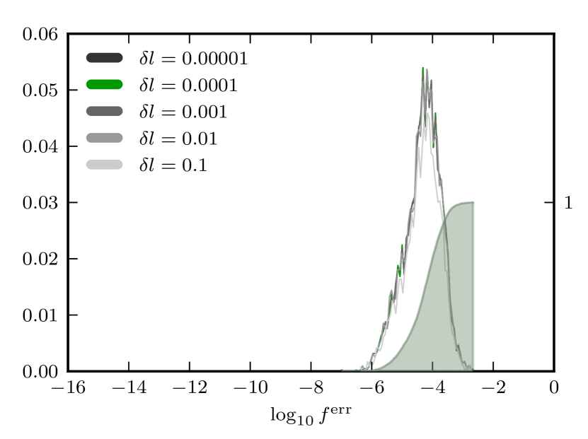
Figure 3: Force error distribution of FMM for the spherical test case without polarization considering different values of the dipole separation distance $\delta l=|\delta\bm{l}|$. Our choice for this approximation makes little difference over 5 orders of magnitude. Here we assume an opening angle of $\theta=0.5$. We highlight in green the $(\alpha,\delta l)=(1,0.0001)$ case presented in Figure 2. The left vertical axis has been normalized such that the area under each curve is 1. Filled curves using the right vertical axis represent the cumulative histograms.

A direct comparison of these parameters with other implementations is difficult as many small details can affect the results. The most robust measure is to demand a maximum error tolerance. We therefore chose for all of our future tests the parameters $\theta=0.5,p=5,|\delta\bm{l}|=0.0001$ Å to ensure a maximum error of $10^{-2}$.

IV.2 Molecular dynamics of a solvated protein complex

We used the Pancreatic Trypsin Inhibitor-Trypsin complex (PDB label 2PTC (Marquart et al., 1983b; Berman et al., 2000)) to test the stability and accuracy of the FMM method used in conjunction with three MD schemes over 1 ns. The protein complex is made of 2 non-bonded proteins and consists of 4,114 atoms (Marquart et al., 1983a). We immersed the system in a single level solvent box made of 28,258 polarizable pseudo-particles (see Figure 4), according to the procedure described in Masella, Borgis, and Cuniasse (2011). As already mentioned, the computations concerning the electrostatic interactions within the protein complex were performed in a non-periodic environment without any cut-off for the atom-atom interactions within the solute and cut-offs at 12 Å and 7 Å for the solvent-solvent and solute-solvent interactions, respectively.

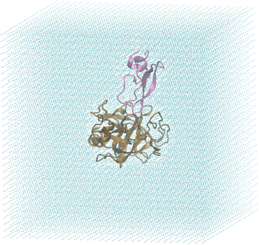
Figure 4: The Pancreatic Trypsin Inhibitor-Trypsin complex (4,114 atoms) immersed in a pseudo-particle solvent (28,258 particles) non-periodic box. We perform six 1 ns simulations of the system to verify our FMM implementation.

Three different integrators were used with both the direct and FMM approaches. The Newtonian equations of motion were solved using 1) the velocity Verlet integrator with 1 fs time steps to handle non-bonded interactions, 2) the same Verlet integrator with 2 fs time steps, and 3) the multiple time step (MTS) integrator devoted to induced dipole moment based potentials (Masella, 2006), where we used a time step of 1 fs for short range non-bonded interactions and 5 fs for long range ones. To handle the quickly varying energy terms (those handling bonded atom interactions), we systematically used a time step of 0.25 fs, regardless of the integrator. Chemical bonds X-H and bending angles H-X-H were constrained to their initial values using the RATTLE algorithm (Andersen, 1983) with a convergence criterion of $10^{-6}$ Å. The induced dipole moments were solved iteratively with a convergence criterion of $10^{-6}$ Debye per polarizable center. However, the iterations continue until the greatest difference between two successive iterations of the induced dipole moment for a single polarizable center is smaller than $20\times 10^{-6}$ Debye. A temperature of 300 K was monitored along the trajectories using the GGMT thermostat (Liu and Tuckerman, 2000) (with a coupling constant of 0.5 ps). The system center of mass kinetic energy was subtracted before a simulation began. Thus, a priori, we expect there to be no drift in the center of mass. Lastly, based on the above spherical tests we use the FMM parameters $\theta=0.5,p=5,|\delta\bm{l}|=0.0001$ Å. All the systems were equilibrated by performing 100 ps runs before starting the 1 ns production runs. The values discussed below were extracted from these simulations.

We observed that the average number of iterations per time step needed to converge the dipole moments using FMM or direct summation differed by about 2%. The small difference originates mainly from the chaotic behavior of the simulation trajectories, which explore different portions of the system potential energy surface.

The total Hamiltonian $H$ (which includes the GGMT thermostat components) for the six 1 ns test cases are presented in the upper plot of Figure 5. The instantaneous total Hamiltonian has been adjusted by the initial value $H_{0}$ and then scaled by the total injected kinetic energy $E_{\mathrm{inject}}^{\mathrm{kin}}$ over the course of the simulation (here $E_{\mathrm{inject}}^{\mathrm{kin}}=$ 63,477 kcal/mol). The initial 100 ps used to equilibrate the system is not shown in the figure.

Because the dipoles are solved iteratively, a small energy drift is expected (Toukmaji et al., 2000) and at the nanosecond scale we observed this mainly for the MTS runs. However, the drifts are small and all clearly under 0.1%. Most importantly, all the FMM runs behave consistently in terms of energy conservation when compared with the direct summation based runs, exhibiting the high precision level of the present FMM implementation. There may be small inaccuracies due to the discontinuity introduced when a particle crosses a cell boundary and transitions from a direct interaction to an FMM one, however, these are largely dominated by errors in the iterative dipole scheme and do not manifest themselves in the final results.

The lower plot of the same figure highlights the conservation of momentum of the full system center of mass. As expected, there is essentially no change in the value over the length of all simulations.

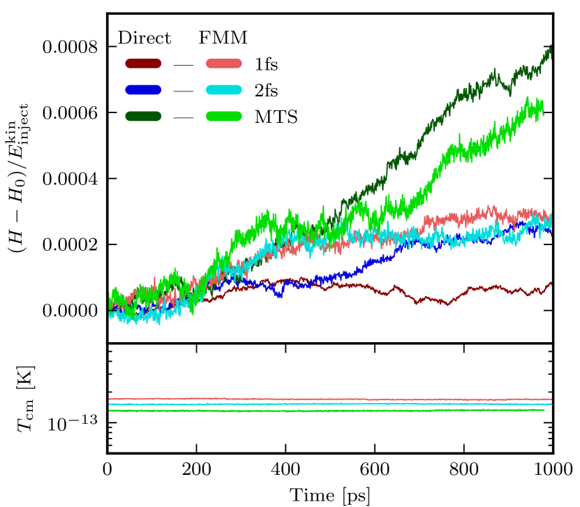
Figure 5: (Top) The energy drift as a fraction of the total injected kinetic energy $E^{\mathrm{kin}}_{\mathrm{inject}}$. For the 2PTC protein simulation using fixed time step and multiple time step integrators $E^{\mathrm{kin}}_{\mathrm{inject}}=$ 63477 kcal/mol. The general behavior using FMM is similar to that of the direct sum computation. (Bottom) The kinetic energy $T_{\mathrm{cm}}$ of the system center of mass with FMM, expressed in Kelvin. The small, nearly constant value for both fixed and multiple time steps demonstrates the expected momentum conserving nature of FMM. The 1 fs and 2 fs data has been offset vertically from the MTS run for clarity.

IV.3 FMM scaling and a comparison with PME

We performed scaling tests using a series of five subset structures of the mature HIV-1 capsid full system recently investigated in liquid water using a PME approach and a non-polarizable standard pairwise force field (Zhao et al., 2013). The molecular structures considered here were extracted from the PDB files 1VU{4–9}. Our base capsid subsystem is an hexamer of the HIV-1 capsid protein. That subsystem contains 21,612 atoms (including hydrogen). Larger capsid subsystems were generated by replicating this base system up to a 5x larger system. Each base hexamer system interacts with the others according to the interaction scheme of the HIV-1 capsid. The largest system considered is thus made of about $10^{5}$ atoms. All computations were performed in vacuum and represent a single energy point computation using the same protocol to solve the dipole moments as for 2PTC and including all short range forces in addition to the long range Coulomb and polarization interactions.

A plot of the FMM scaling and speedup compared with direct summation is shown in Figure 6. For the scaling, we consider just the time to perform the electrostatic force and electric field (ES/EF) calculation. This isolates the FMM algorithm from other computations. The FMM implementation clearly scales linearly with the size of the system as indicated by the solid line. The speedup plot compares FMM to a direct summation computation. Here, we show the speedup both for the isolated ES/EF calculation and for a complete timestep. We find that FMM is about 7 times faster than the direct method for the largest capsid system, although for the smallest system the two methods are nearly comparable. Table 1 provides the absolute timings used in the plot.

To efficiently simulate a molecular system (using free or periodic boundary conditions), one may also consider a PME approach. To evaluate if an FMM approach can be competitive to handle large molecular systems when accounting for polarization, we also provide timing information for the capsid systems when using the PME implementation in Polaris(MD), which is based on the most efficient PME approach proposed in Darden, York, and Pedersen (1993) and the work of Toukmaji et al. (2000) for induced dipole moment-based force-fields. The fast Fourier transform is performed using the FFTW 3.3.4 library (Frigo and Johnson, 2005), with SIMD vectorization enabled; most of the Polaris(MD) loops involved in the PME energy/analytical gradient computations have also been vectorized. For consistency, we restricted the iterative scheme to solve the induced dipole moments with 10 iterations, regardless of the computational protocol used. This is the upper bound of the number of iterations needed to achieve the dipole convergence along a trajectory when considering the convergence criteria used for the 2PTC system.

We considered three typical grid sizes of 0.5 Å (high resolution), 1 Å (medium resolution) and 2 Å (low resolution). The PME direct energy terms were truncated for inter-atomic distances larger than 12 Å. When considering the latter cutoff distance and a 1 Å grid size, the PME precision corresponds to truncating the direct and reciprocal standard Ewald sums for terms smaller than 10^-8 (Mazars, 2011, and references therein). This is considered a high level of precision for Ewald (see e.g., Toukmaji et al., 2000). The capsid systems were set in their inertial frame of reference and the size of the enclosing boxes correspond to the largest capsid coordinate in each dimension plus $\sim$10 Å (see §B). We ensured that the dimension values had small prime factors to take advantage of optimizations in the FFT library.

For FMM, we used the parameters $\theta=0.5,p=5,|\delta\bm{l}|=0.0001$ Å, corresponding to a force accuracy where about 80% of the relative error is less than $10^{-4}$ and no more than $10^{-2}$. For a complete timestep, the order of magnitude of the FMM timings is comparable to PME when using a grid size of 1 Å, but PME is faster than FMM by a factor of $\sim$3, regardless of the capsid system size. PME is significantly faster, however, for the ES/EF computations, up to a factor $\sim$10. The reason for the efficiency gain made by FMM for a complete timestep is that while PME maintains the same grid for the dipole convergence, FMM is able to build a more efficient tree using only the dipole sites, which are about three times less than the total number of atoms when using the polarizable force-field implemented in Polaris(MD). Given further optimizations in our FMM implementation, we may reasonably expect the FMM/PME gap to be smaller in the near future. The present FMM implementation represents thus an interesting alternative to account for electrostatic/polarization long range interactions when modeling large molecular systems at the microscopic level. In particular, we may note here that the FMM timings for an opening angle $\theta=0.7$ match almost perfectly the PME timings for a grid size of 1 Å (results not shown in Table 1). Moreover, compared to using a high resolution PME grid size of 0.5 Å, the current FMM implementation is clearly faster by a factor of a few.

	Direct [s]			FMM [s]			PME 0.5Å [s]			PME 1Å [s]			PME 2Å [s]
No. Atoms	ES/EF	Dipole	Complete	ES/EF	Dipole	Complete	ES/EF	Dipole	Complete	ES/EF	Dipole	Complete	ES/EF	Dipole	Complete
21612	$2.11$	$4.29$	$8.43$	$1.44$	$4.00$	$6.71$	$0.16$	$16.12$	$18.45$	$0.17$	$1.37$	$2.17$	$0.16$	$0.52$	$1.21$
43224	$8.36$	$17.02$	$33.40$	$2.87$	$7.99$	$13.38$	$0.33$	$20.44$	$23.92$	$0.33$	$3.56$	$5.22$	$0.33$	$1.12$	$2.50$
64836	$18.98$	$39.66$	$77.87$	$4.59$	$13.24$	$21.87$	$0.50$	$31.36$	$36.67$	$0.50$	$5.71$	$8.25$	$0.49$	$1.71$	$3.79$
86448	$34.39$	$69.05$	$138.52$	$5.93$	$16.74$	$27.51$	$0.66$	$48.01$	$55.70$	$0.67$	$7.29$	$10.63$	$0.67$	$2.35$	$5.16$
108060	$54.70$	$108.02$	$218.27$	$7.49$	$20.52$	$34.62$	$0.82$	$68.21$	$79.49$	$0.82$	$10.20$	$14.48$	$0.82$	$3.15$	$6.64$

Table 1: Timing measurements (in seconds) for the capsid systems using direct summation, FMM, and PME. For each method we measured the time to complete the electrostatic (ES/EF) calculation, the dipole convergence step, and the complete timestep, which includes some additional computation. For the PME approach, we used three typical grid sizes of 0.5 Å (high resolution), 1 Å (medium resolution) and 2 Å (low resolution). The analysis was performed on a single core of an Intel Core i7 1.7GHz CPU.

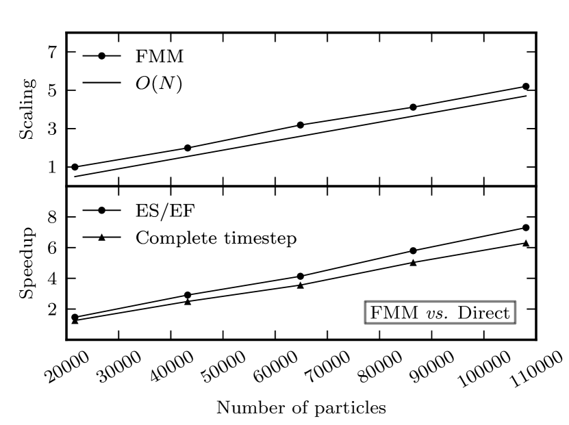
Figure 6: Performance properties of FMM with the HIV capsid subsystem for increasing system size. (Top) The relative scaling of FMM (normalized by the smallest system), for the electrostatic/electric-field (ES/EF) calculation. The line labeled $O(N)$ represents perfect linear scaling. (Bottom) The speed up of FMM over direct summation when calculating either ES/EF or a complete timestep, which also includes the dipole convergence step. Detailed timing information can be found in Table 1.

V Conclusions

We have implemented a momentum conserving version of the fast multipole method in the molecular dynamics code Polaris(MD) and demonstrated the applicability of FMM by combining it with state-of-the-art chemical models to compute, in $O(N)$ time, Coulomb forces and polarization interactions associated with the induced dipole polarization method. Through a series of artificial and real-world test cases—most notably, recent HIV-1 capsid subsystems from Zhao et al. (2013)—we have shown that we are able to achieve very good accuracy by combining a multipole expansion to $5^{\mathrm{th}}$ order and an opening angle tolerance criteria of $\theta=0.5$. During 1 ns MD simulations of the 2PTC protein, we observe an energy drift of less than 0.1% of the total kinetic energy injected in the system and observe no change in the total momentum—both consistent with standard $O(N^{2})$ direct summation-based simulations.

Performance measurements using the HIV capsid subsystems have demonstrated that FMM can be $\sim$7 times faster than the direct summation method for systems of about $10^{5}$ atoms. When accounting for polarization, the unoptimized FMM routines are only a factor of a few slower than a PME approach using a 1 Å grid size and a factor of a few faster than PME with a grid size of 0.5 Å. Since FMM is expected to scale better than FFT-based approaches, such as PME, particularly on forthcoming supercomputer architectures, it may prove to be the method of choice for extremely large molecular dynamics simulations of the future.

Appendix A Additional 2PTC tests

In Figure 7 we show the distribution of errors after a single energy calculation of 2PTC. The distribution is remarkably similar to the spherical tests with a peak in log-space just below $10^{-4}$. In addition, we present in Figure 8 the temporal evolution of the system potential energy $E^{\mathrm{pot}}$ over the course of the 1 ns simulations. For each simulation, an initial 100 ps was used to relax the system using the same procedure as the production phase (not shown in the figure). This results in slightly different initial conditions for each run, as seen by a different initial value of $E_{\mathrm{pot}}$. Therefore, this plot shows that different portions of the system potential energy surface are explored along each trajectory, and explains the difference in the number of iterations needed to converge the dipole in direct sum and FMM simulations. The original data has been smoothed with a Hanning filter for clarity and to reduce the noise.

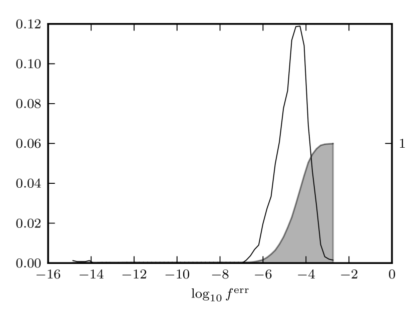
Figure 7: Force error distribution of FMM after one time step of the 2PTC protein complex compared with a direct sum calculation. The left vertical axis has been normalized such that the area under the curve is 1. The filled curve using the right vertical axis represents the cumulative histogram.

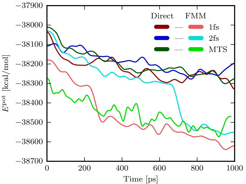
Figure 8: The potential energy $E^{\mathrm{pot}}$ for the six 1 ns simulations of the 2PTC protein complex. The drift is due to the presence of chaotic effects in the MD trajectories. The original data has been smoothed with a Hanning filter for clarity and to reduce the noise.

Appendix B Grid sizes for PME

The dimensions of the boxes, in which the capsid systems are embedded, are $112\times 120\times 128$, $104\times 136\times 224$, $112\times 136\times 320$, $120\times 140\times 406$, and $140\times 140\times 496$ for the PME simulations with a grid spacing of 1 Å. All dimensions in Å. For the grid spacing of 0.5 Å the dimensions are twice these values, and for the grid spacing of 2.0 Å they are half of these values to maintain the same physical box size.

Appendix C Generating the multipole expansions

Computing multipoles to order $p=5$ is a non-trivial task to perform by hand. We have instead implemented a program in Python (Rossum, 1995) that symbolically generates the code for all FMM operations. The equations are then symbolically simplified using the SymPy library (SymPy Development Team, 2014). By eliminating common subexpressions we see up to a ten fold decrease in operation count, although scaling still behaves as $O(p^{4})$.

Appendix D Multi-index notation

The multi-index notation simplifies the tensor representation in the derivation of the FMM operations. Following from property (24) addition and subtraction operations are only valid for those tuples that have all $n_{i}\geq 0$.

$$\bm{\mathsf{n}} = (n_{x},n_{y},n_{z})\mathrm{\ where\ }n_{i}\geq 0$$ (24)

$$|\bm{\mathsf{n}}| \equiv n_{x}+n_{y}+n_{z}$$ (25)

$$\bm{\mathsf{n}}! \equiv n_{x}!\;n_{y}!\;n_{z}!$$ (26)

$$\bm{\mathsf{n}}\pm k \equiv (n_{x}\pm k,n_{y}\pm k,n_{z}\pm k)$$ (27)

$$\bm{\mathsf{n}}\pm\bm{\mathsf{m}} \equiv (n_{x}\pm m_{x},n_{y}\pm m_{y},n_{z}\pm m_{z})$$ (28)

$$\bm{r}^{\bm{\mathsf{n}}} \equiv r_{x}^{n_{x}}\,r_{y}^{n_{y}}\,r_{z}^{n_{z}}$$ (29)

References

- Andersen (1983) Andersen, H. C., Journal of Computational Physics 52, 24 (1983).
- Arnold et al. (2013) Arnold, A., Fahrenberger, F., Holm, C., Lenz, O., Bolten, M., Dachsel, H., Halver, R., Kabadshow, I., Gähler, F., Heber, F., Iseringhausen, J., Hofmann, M., Pippig, M., Potts, D., and Sutmann, G., Phys. Rev. E 88, 063308 (2013).
- Barnes and Hut (1986) Barnes, J. and Hut, P., Nature (London) 324, 446 (1986).
- Berman et al. (2000) Berman, H. M., Westbrook, J., Feng, Z., Gilliland, G., Bhat, T. N., Weissig, H., Shindyalov, I. N., and Bourne, P. E., Nucleic Acids Research 28, 235 (2000).
- Bishop, Skeel, and Schulten (1997) Bishop, T. C., Skeel, R. D., and Schulten, K., Journal of Computational Chemistry 18, 1785 (1997).
- Chang and Dang (2006) Chang, T.-M. and Dang, L. X., Chem. Rev. 106, 1305 (2006).
- Cieplak et al. (2009) Cieplak, P., Dupradeau, F.-Y., Duan, Y., and Wang, J., J. Phys.: Condens. Matter 21, 333102 (2009).
- Dang (2000) Dang, L., J. Chem. Phys. 113, 266 (2000).
- Darden, York, and Pedersen (1993) Darden, T., York, D., and Pedersen, L., J. Chem. Phys. 98, 10089 (1993).
- Dehnen (2002) Dehnen, W., Journal of Computational Physics 179, 27 (2002).
- Dehnen (2014) Dehnen, W., Computational Astrophysics and Cosmology 1, 1 (2014).
- Diemand et al. (2008) Diemand, J., Kuhlen, M., Madau, P., Zemp, M., Moore, B., Potter, D., and Stadel, J., Nature (London) 454, 735 (2008).
- Figueirido et al. (1997) Figueirido, F., Levy, R. M., Zhou, R., and Berne, B. J., The Journal of Chemical Physics 106, 9835 (1997).
- Frigo and Johnson (2005) Frigo, M. and Johnson, S. G., Proceedings of the IEEE 93, 216 (2005).
- Greengard and Rokhlin (1987) Greengard, L. and Rokhlin, V., Journal of Computational Physics 73, 325 (1987).
- Ha-Duong et al. (2002) Ha-Duong, T., Phan, S., Marchi, M., and Borgis, D., J. Chem. Phys. 117, 541 (2002).
- Jungwirth and Tobias (2006) Jungwirth, P. and Tobias, D. J., Chem. Rev. 106, 1259 (2006).
- Liu and Tuckerman (2000) Liu, Y. and Tuckerman, M. E., J. Chem. Phys. 112, 1685 (2000).
- Lopes, Roux, and MacKerell Jr (2009) Lopes, P., Roux, B., and MacKerell Jr, A., Theor. Chem. Acc. 124, 11 (2009).
- Marquart et al. (1983a) Marquart, M., Walter, J., Deisenhofer, J., Bode, W., and Huber, R., Acta Crystallogr. Sect.B 39, 480 (1983a).
- Marquart et al. (1983b) Marquart, M., Walter, J., Deisenhofer, J., Bode, W., and Huber, R., Acta Crystallographica Section B 39, 480 (1983b).
- Masella (2006) Masella, M., Molecular Physics 104, 415 (2006).
- Masella, Borgis, and Cuniasse (2008) Masella, M., Borgis, D., and Cuniasse, P., Journal of Computational Chemistry 29, 1707 (2008).
- Masella, Borgis, and Cuniasse (2011) Masella, M., Borgis, D., and Cuniasse, P., Journal of Computational Chemistry 32, 2664 (2011).
- Masella, Borgis, and Cuniasse (2013a) Masella, M., Borgis, D., and Cuniasse, P., Journal of Computational Chemistry 34, 1112 (2013a).
- Masella, Borgis, and Cuniasse (2013b) Masella, M., Borgis, D., and Cuniasse, P., Journal of Computational Chemistry 34, 1112 (2013b).
- Masella and Cuniasse (2003) Masella, M. and Cuniasse, P., The Journal of Chemical Physics 119, 1866 (2003).
- Mazars (2011) Mazars, M., Physics Reports 500, 43 (2011).
- Perram, Petersen, and De Leeuw (1988) Perram, J. W., Petersen, H. G., and De Leeuw, S. W., Molecular Physics 65, 875 (1988).
- Réal et al. (2013) Réal, F., Trumm, M., Schimmelpfennig, B., Masella, M., and Vallet, V., J. Comput. Chem. 34, 707 (2013).
- Rossum (1995) Rossum, G., “Python reference manual,” Tech. Rep. (Amsterdam, The Netherlands, 1995).
- Sagui and Darden (1999) Sagui, C. and Darden, T. A., Annual Review of Biophysics and Biomolecular Structure 28, 155 (1999).
- Salanne and Madden (2011) Salanne, M. and Madden, P., Mol. Phys. 109, 2299 (2011).
- Scarpazza et al. (2013) Scarpazza, D., Ierardi, D., Lerer, A., Mackenzie, K., Pan, A., Bank, J., Chow, E., Dror, R., Grossman, J., Killebrew, D., Moraes, M. A., Predescu, C., Salmon, J., and Shaw, D., IEEE 27th International Symposium on Parallel and Distributed Processing 35, 933 (2013).
- Stadel et al. (2009) Stadel, J., Potter, D., Moore, B., Diemand, J., Madau, P., Zemp, M., Kuhlen, M., and Quilis, V., Mon. Not. Roy. Astron. Soc. 398, L21 (2009).
- SymPy Development Team (2014) SymPy Development Team,, SymPy: Python library for symbolic mathematics (2014), available at http://www.sympy.org.
- Thole (1981) Thole, B. T., Chemical Physics 59, 341 (1981).
- Toukmaji et al. (2000) Toukmaji, A., Sagui, C., Board, J., and Darden, T., The Journal of Chemical Physics 113, 10913 (2000).
- Wang and Skeel (2005) Wang, W. and Skeel, R. D., The Journal of Chemical Physics 123, 164107 (2005).
- Yokota and Barba (2012) Yokota, R. and Barba, L. A., Int. J. High Perform. Comput. Appl. 26, 337 (2012).
- Zhao et al. (2013) Zhao, G., Perilla, J. R., Yufenyuy, E. L., Meng, X., Chen, B., Ning, J., Ahn, J., Gronenborn, A. M., Schulten, K., Aiken, C., and Zhang, P., Nature 497, 643 (2013).