Efficient solution of structural default models with correlated jumps and mutual obligations

Abstract

The structural default model of Lipton and Sepp, (2009) is generalized for a set of banks with mutual interbank liabilities whose assets are driven by correlated Lévy processes with idiosyncratic and common components. The multi-dimensional problem is made tractable via a novel computational method, which generalizes the one-dimensional fractional partial differential equation method of Itkin, 2014a to the two- and three-dimensional cases. This method is unconditionally stable and of the second order of approximation in space and time; in addition, for many popular Lévy models it has linear complexity in each dimension. Marginal and joint survival probabilities for two and three banks with mutual liabilities are computed. The effects of mutual liabilities are discussed, and numerical examples are given to illustrate these effects.

1 Introduction

Structural default framework is widely used for assessing credit risk of rate debt. Introduced in its simplest form in a seminal work Merton, (1974), this framework was further extended in various papers, see a survey in Lipton and Sepp, (2011) and references therein. In contrast to reduced-form models, structural default models suffer from the curse of dimensionality when the number of counterparties grows; however, these models provide a more natural financial description of the default event for a typical firm.

One of the possible extensions of the structural framework, which is of high importance in the current environment, consists in taking into account the fact that banks, in addition to their liabilities to the outside economy, also have some liabilities to each other. This topic is discussed, e.g., in Webber and Willison, (2011), where it is mentioned that systemic capital requirements for individual banks, determined as the solution to the policymaker’s optimization problem, depend on the structure of banks’ balance sheets (including their obligations to other banks) and the extent to which their asset values tend to move together. More generally, systemic capital requirements are found to be increasing in banks’ balance sheet size relative to other banks in the system, as well as their interconnectedness, and, materially, contagious bankruptcy costs.

From this perspective, an extension of the simplest Merton model can be proposed to quantify default risks in an interconnected banking system. For instance, Elsinger et al., (2006), Gauthier et al., (2010) consider systemic risk in such a system and attribute it either to correlations between the asset values of the banks, or to interlinkages of the banks’ balance sheets, which could result in contagious defaults. An extended Merton model can be built as a combination of the correlated Merton balance sheet models, calibrated by using observed bank equity returns, and a network of interbank exposures cleared in the spirit of Eisenberg and Noe, (2001).

In this paper we develop a model, which builds upon its predecessors; yet, it differs from the earlier models in one very important respect. Namely, rather than addressing a point-in-time default event, we consider defaults, which can occur at any time, by introducing a continuous default barrier in the spirit of Black and Cox, (1976). We feel that this extension is necessary in order to analyze the effect of mutual liabilities properly, especially because we wish to provide not just qualitative, but also quantitative conclusions. To avoid confusion, we emphasize that this effect differs from that of contagion for correlated defaults in reduced-form models, see, e.g., Yu, (2007), Bielecki et al., (2011).

To achieve our goal, we need to come up with a suitable structural model capable of handling mutual obligation effects at various time scales. It is well-known that pure diffusion asset dynamics is manifestly inadequate for relatively short time-scales, and we need to introduce jumps into the model, see, e.g., Zhou, (2001), Lipton, 2002b . Therefore, we choose a Lévy jump-diffusion driver for the asset dynamics.

Multi-dimensional Lévy processes find various applications in mathematical finance. They are used in modeling basket equity derivatives, various credit derivatives, etc. Unfortunately, tractability of multi-dimensional Lévy processes is rather limited. In addition, it is difficult to study such processes because they suffer from the curse of dimensionality. Various numerical methods, including analytical, semi-analytical, finite-difference (FD), Monte-Carlo methods, and their combinations have been used for solving the corresponding problems, again see, e.g., a survey in Lipton and Sepp, (2011) and references therein. Certainly, rather straightforward Monte Carlo method can be proposed to simulate multi-dimensional Lévy processes. However, in general it is both slow or inaccurate. Therefore, finite difference methods seem to be a viable alternative for 2D and 3D problems, despite the fact that in the 3D case such methods can be relatively slow (but definitely faster than the corresponding Monte Carlo method).

The authors are aware of limited number of papers on mathematical finance, which are using FD methods to solve 2D partial Integro-differential equation (PIDE) describing the evolution of two fully correlated assets, see, e.g., Clift and Forsyth, (2008), Lipton and Sepp, (2009, 2011). In Clift and Forsyth, (2008), the authors use a bivariate distribution proposed in Marshall and Olkin, (1967) and consider normal and exponentially distributed multivariate jumps. In Lipton and Sepp, (2009), the authors consider assets, which are correlated twofold. First, diffusion components are correlated in the standard manner because they are driven by correlated Brownian motions. Second, jump components are correlated because for each asset they are represented as a sum of a) systemic exponential jumps common for all assets, and b) idiosyncratic exponential jumps specific for a particular asset. From a historical perspective, this idea can be traced back to the work of Vasicek, who developed a multi-factor structural model assuming that the dynamics of individual assets can be described as a sum of systemic and idiosyncratic parts, Vasicek, (1987, 2002) .

However, other Lévy models could be of interest as well, see, e.g., Eberlein and Keller, (1995), where it is shown that generalized hyperbolic models fit the market data pretty well. Therefore, an extended framework which allows for general Lévy models to be used when modeling jumps is highly desirable. Below we provide a short survey of various approaches to introduce multivariate correlated jumps via Lévy’s copula, multivariate subordinators of the Brownian motion, etc., as well as discuss their advantages and pitfalls. Our main concerns with regard to the existing approaches are two-fold: a) some of them are not flexible enough to meet all the modeling requirements, because they impose some undesirable restrictions on the jump correlation structure; b) they suffer from the curse of dimensionality in the sense that their complexity is polynomial rather than linear in each dimension.

Another observation is that even in the 1D case traditional methods for solving PIDEs experience some problems, see a survey in Itkin, 2014a , and references therein. In the multi-dimensional case these problems become even harder. To deal with these problems, we choose a particular way of introducing correlated jumps and combine it with the multi-dimensional version of the matrix exponential method proposed first in Itkin and Carr, (2012) and later further elaborated in Itkin, 2014a , Itkin, 2014c . The presented construction allows different jumps to be used for modeling the idiosyncratic and common factors. For example, in the 2D case we can represent idiosyncratic jumps of the first bank by using the Meixner model of Schoutens, (2001), idiosyncratic jumps of the second bank by using the Merton model, and simulate their common jumps by using the CGMY model. We do not claim that such rich choice of Lévy processes is necessary in practice, since the actual jump distribution is hard to establish with certainty, merely that it is possible to do. In our experience, hyper-exponential jumps introduced in Lipton, 2002b are more than adequate for all practical purposes. We don’t consider every possible combination of Lévy processes in this paper, since this could be done based on the general principles described in Itkin, 2014a , Itkin, 2014c . However, as an example, we do consider a model with Gaussian idiosyncratic jumps and exponential systemic jumps. As part of this example, we think of idiosyncratic jumps as two-sided, while systemic jumps as one-sided. In this sense, our example should be ideologically similar to that in Clift and Forsyth, (2008). However, our method is not restricted by this choice and differs from that of Clift and Forsyth, (2008) in several important respects: a) we use Gaussian and exponential jumps just as an example, other common jumps and univariate marginals could be used as well; b) we use the matrix exponential method, rather than the traditional method for solving the corresponding PIDE; c) we present a splitting method to provide solutions of the 2D and 3D problems with second order of accuracy in both space and time, and prove convergence of the method. Our method is of the linear complexity (i.e., $O(N_{1}\times N_{2})$ in the 2D case and $O(N_{1}\times N_{2}\times N_{3})$ in the 3D case) provided that the Merton, Kou, CGMY or Meixner Lévy models are used. Our method is faster than the FFT method used in Clift and Forsyth, (2008).

In this paper, we concentrate on our structural default model for two or three banks with mutual liabilities. The method can also be used to price basket options. We show that accounting for these liabilities affects both the joint survival probability of these banks, which is to be expected, as well as their marginal survival probabilities, which is not the case when mutual liabilities are ignored. This fact has to be taken into account when marginals are calibrated to the market CDS spreads. We provide several numerical examples in order to demonstrate that the presence of mutual obligations could potentially strongly affect the corresponding survival probabilities, and, by implication, the stability of the inter-bank system, especially in the 3D case.

The new results of the paper are as follows: a) interbank mutual obligations are incorporated in the structural default credit model with correlated jumps, and their impact on the joint and marginal probabilities is investigated both qualitatively and quantitatively; b) new splitting method is proposed to solve the corresponding PIDE with correlated jumps in the 2D and 3D cases. The method includes new steps that don’t appear in the 1D case. For many popular Lévy models the method provides linear complexity in each dimension and is unconditionally stable.

The rest of the paper is organized as follows. In section 2 we describe our multi-dimensional structural model, which is an extension of Lipton and Sepp, (2009). In section 3 we provide a short survey of the existing approaches to multivariate correlated jumps, and describe the one we find to be particularly suitable for our goals. In section 4 we shortly describe the method of Itkin and Carr, (2012), Itkin, 2014a , Itkin, 2014c and extend it to the multi-dimensional case. In section 5 we describe the splitting algorithm, which is adopted for solving the corresponding multi-dimensional PIDE. In section 6 we provide a detailed numerical scheme for solving the fractional jump equations and prove the unconditional stability, second order accuracy and convergence of the scheme. We also emphasize that our scheme preserves positivity of the solution. The results of our numerical experiments are discussed in sections 7 (the 2D case) and 8 (the 3D case). In section 8, we describe necessary details of the numerical scheme used in the 3D case. We draw our conclusions in section 9.

2 Interbank mutual obligations in a structural default model

Similar to Lipton and Sepp, (2009, 2011) we consider a multi-dimensional structural model inspired by the familiar model of Merton, (1974), see Lipton and Sepp, (2009, 2011) and references therein.

First, for simplicity, assume that we have just two banks with external assets $A_{i,t}$, $i=1,2$ and liabilities $L_{i,t}=G_{t}L_{i,0}$, and no mutual liabilities. Here $G_{t}$ is the deterministic growth factor

$$G_{t}=\exp\left(\int_{0}^{t}r_{t^{\prime}}dt^{\prime}\right),$$ (1)

where $r_{t}$ is the forward rate. Also assume that the default barrier $l_{i,t}$ is a deterministic function of time:

$$l_{i,t}=\begin{cases}R_{i}L_{i,t},&t<T,\\ L_{i,T},&t=T,\end{cases}$$

where $R_{i}$ is the average recovery of the bank’s liabilities, and $T$ is the debt maturity. Under normal circumstances, $R_{i}$ has a typical value $R_{i}=0.4$.

We define the $i$th bank’s default time $\tau_{i}$ assuming continuous monitoring as follows

$$\tau_{i}=\inf_{0<t\leq T}[A_{i,t}\leq l_{i,t}].$$

Let us extend this approach by assuming that the banks in question do have mutual liabilities, which we denote by $L_{ij,t},\ i,j=1,2$; below we assume that $L_{ij,t}=G_{t}L_{ij,0}$. Thus, the total assets and liabilities of the $i$th bank are $A_{i}+\sum_{j\neq i}L_{ji}$ and $L_{i}+\sum_{j\neq i}L_{ij}$, respectively. Accordingly, the default time of the first bank has the form

$$\tau_{1}=\inf_{0<t\leq T}[A_{1,t}\leq\lambda_{1,t}],$$ (2)

where

$$\lambda_{1,t}=\begin{cases}R_{1}\left(L_{1,t}+L_{12,t}\right)-L_{21,t},&t<T,\\ L_{1,T}+L_{12,T}-L_{21,T},&t=T.\end{cases}$$

The default time of the second bank has a similar form

$$\tau_{2}=\inf_{0<t\leq T}[A_{2,t}\leq\lambda_{2,t}].$$ (3)

A new situation occurs, however, in case of default of one of the banks. In case when the second bank defaults, it pays back to its creditors only a portion of its liabilities, namely $R_{2}(L_{2}+L_{21})$. However, the first bank pays back to the successors of the second bank the full amount $L_{12}$, assuming of course that it does not default simultaneously with the second bank. Thus, at time $\tau_{2}$ the first bank receives from the second bank the amount $R_{2}L_{21}$ and pays the amount $L_{12}$. Therefore, the new asset value $\tilde{A}_{1}$ of the first bank becomes $\tilde{A}_{1}=A_{1}+R_{2}L_{21,\tau_{2}}-L_{12,\tau_{2}}$, while its liability value becomes $L_{1,\tau_{2}}$. We assume that the actual external assets do not jump in value, while the outside liabilities do get adjusted. If the amount $R_{2}L_{21,\tau_{2}}-L_{12,\tau_{2}}$ is positive, i.e., the first bank gets extra cash, which it spends retiring some of the external liabilities. If this amount is negative, then it is borrowed from the external sources. In both cases the total external liabilities become

$$\tilde{L}_{1,\tau_{2}}=L_{1,\tau_{2}}-R_{2}L_{21,\tau_{2}}+L_{12,\tau_{2}}.$$

Accordingly, the new default barrier for the first bank could be defined as

$$\tilde{\lambda}_{1,t}=+\begin{cases}\lambda_{1,t},&t<\tau_{2},\\ \bar{\lambda}_{1,t},&t\geq\tau_{2},\end{cases}\qquad\bar{\lambda}_{1,t}=\begin{cases}R_{1}\left(L_{1,\tau_{2}}-R_{2}L_{21,\tau_{2}}+L_{12,\tau_{2}}\right)G_{t}/G_{\tau_{2}},&t<T,\\ (L_{1,\tau_{2}}-R_{2}L_{21,\tau_{2}}+L_{12,\tau_{2}})G_{T}/G_{\tau_{2}},&t=T,\end{cases}$$

so that its default time has the form

$$\tilde{\tau}_{1}=\inf_{0<t\leq T}[A_{1,t}\leq\tilde{\lambda}_{1,t}]..$$ (4)

It is easy to see, that after the default of the second bank, the default boundary of the first bank increases by the amount of

$$\Delta\lambda_{1,\tau_{2}}=\tilde{\lambda}_{1,\tau_{2}}-\lambda_{1,\tau_{2}}=(1-R_{1}R_{2})L_{21,\tau_{2}}>0.$$ (5)

Similarly,

$$\Delta\lambda_{2,\tau_{1}}=(1-R_{1}R_{2})L_{12,\tau_{1}}>0.$$ (6)

Thus, the default boundary of the first bank jumps up by the increment $\Delta\lambda_{1}$ at time $\tau_{2}$, and the default boundary of the second bank jumps up by the increment $\Delta\lambda_{2}$ at time $\tau_{1}$. Mathematically, this means that our problem now has floating boundaries that are deterministic functions of time which could increase at some moment by jumping to a higher value.

Figure 1: Default boundaries of two banks with and without mutual liabilities.

To illustrate the above observation, let us consider Fig. 1 where the situation is depicted at some moment of time $t<T$. If we don’t take into account mutual liabilities $L_{12}$ and $L_{21}$, then the default boundaries are: for the first bank - a vertical line along the path ”5-2-3-6”; for the second bank - a horizontal line along the pass ”9-3-7-4”. In the presence of mutual liabilities, the default boundary for the first bank becomes ”5-2-3-7-8”, while for the second bank it has the form ”1-2-3-7-4”.

A similar consideration can be used to show that the calculation of the marginal survival probabilities (which are needed to calibrate the model to the market CDS spreads) is strongly impacted by mutual liabilities. To emphasize this point, again consider the domain in Fig 1. Suppose we need to know $q_{1}(A_{1},A_{2},t,T)$ which is the marginal survival probability of the first bank conditional on the asset value $A_{2}$ of the second bank. In the presence of interbank liabilities we observe a new situation since the dynamics the first bank depends on the possible default of the second bank via the boundary conditions. Hence, the problem of computing $q_{1}$ remains inherently two-dimensional in contrast to the situation with no interbank liabilities.

In what follows we provide some numerical results that demonstrate this behavior in the case of two and three firms by solving the corresponding 2D and 3D PIDEs describing the evolution of both joint and survival probabilities in time and space. We also discuss how parameters of the model affect the magnitude of the effect.

To proceed further, we need to specify the dynamics of the external risky assets $A_{1,t},A_{2,t}$; we assume that it could include both diffusion and jumps components. We also assume that these assets are correlated as follows:

1. Diffusion components are correlated with the correlation coefficient $\rho$.

2. Jumps are correlated with the correlation coefficient $\rho_{1,2}$ (see below for a more precise definition of this correlation coefficient).

3. Changes in the firm value due to jumps and diffusion are uncorrelated.

We assume that the underlying asset prices $A_{i,t}$ are driven by exponential Lévy processes

$$A_{i,t}=A_{i,0}\exp(\Lambda_{i,t}),\quad 0\leq t\leq T,$$ (7)

Under an appropriate pricing measure, each $\Lambda_{i,t}$ is characterized by a Lévy triplet $\left(\gamma_{i},\sigma_{i},\nu_{i}\right)$ with the drift $\gamma_{i}$, volatility $\sigma_{i}$, and Lévy measure $\nu_{i}$,

$$\Lambda_{i,t}=\gamma_{i}+\sigma_{i}W_{i,t}+Y_{i,t},\qquad\gamma_{i},\sigma_{i}\in\mathbb{R},\quad\sigma_{i}>0,$$ (8)

where $W_{t}$ is a standard Brownian motion on $0\leq t\leq T$ and $Y_{t}$ is a pure jump process. We consider this process under the pricing measure, therefore, $A_{i,t}/G_{t}$ is a martingale. This allows us to express $\gamma$ as (Eberlein, (2009)) (further on we omit sub-index $i$ for simplicity)

$$\gamma=r-\frac{\sigma^{2}}{2}-\int_{\mathbb{R}}\left(e^{x}-1-x\mathbf{1}_{|x|<1}\right)\nu(dx),$$

with

$$\int_{|x|>1}e^{x}\nu(dx)<\infty.$$

At this stage, the jump measure $\nu(dx)$ is left unspecified, because we are open to consider all types of jumps including those with finite and infinite variation, and finite and infinite activity.

Let us introduce the logarithmic variables $x_{i}=\log A_{i}$ and define the joint survival probability as follows

$$Q(x_{1},x_{2},t,T)=\mathbf{1}_{\tau_{1}>t,\tau_{2}>t}E_{t}^{Q}[\mathbf{1}_{\tau_{1}>T,\tau_{2}>T}].$$

The joint survival probability solves the following PIDE, see Lipton and Sepp, (2011) and also Clift and Forsyth, (2008)

$$Q_{\tau}=[\mathcal{L}+\mathcal{J}]Q,$$ (9)

where $\tau=T-t$ is the backward time, and $\mathcal{L}$ is the two-dimensional linear convection-diffusion operator of the form

$$\mathcal{L}=\sum_{i=1}^{2}\left(r-\frac{\displaystyle 1}{\displaystyle 2}\sigma^{2}_{i}\right)\frac{\partial}{\partial x_{i}}+\frac{\displaystyle 1}{\displaystyle 2}\sum_{i,j=1}^{2}\rho_{i,j}\sigma^{2}_{i}\sigma^{2}_{i}\frac{\partial}{\partial x_{i}}\frac{\partial}{\partial x_{j}},$$ (10)

and $\mathcal{J}$ is the jump operator

$$\mathcal{J}Q=\int_{-\infty}^{\infty}\Big{[}Q(x_{1} +y_{1},x_{2}+y_{2},\tau)-Q(x_{1},x_{2},\tau)-(e^{y_{1}}-1)\frac{\partial Q(x_{1},x_{2},\tau)}{\partial x_{1}}$$ (11)

$$-(e^{y_{2}}-1)\frac{\partial Q(x_{1},x_{2},\tau)}{\partial x_{2}}\Big{]}\nu(dy_{1}dy_{2}),$$

where $\nu(dy_{1}dy_{2})$ is the two-dimensional Lévy measure.

This PIDE has to be solved subject to the boundary and terminal conditions. The terminal condition reads

$$Q(x_{1},x_{2},0)=\mathbf{1}_{x_{1}>\log\tilde{\lambda}_{1}(0),\ x_{2}>\log\tilde{\lambda}_{2}(0)}.$$

The boundary conditions could be set as the Dirichlet conditions at $\pm\infty$. Obviously,

$$Q(x_{1},x_{2},\tau)\rightarrow 0,\ \mbox{at}\ x_{i}\rightarrow-\infty.$$

As $x_{i}\rightarrow\infty,\ i=1,2$, $Q(x_{1},x_{2},\tau)$ should replicate the marginal survival probability $Q(x_{3-i},\tau)$. This condition, however, must be supplemented with the boundary condition when both $x_{1}\rightarrow\infty$ and $x_{2}\rightarrow\infty$. A natural choice is $Q(x_{1}\rightarrow\infty,x_{2}\rightarrow\infty,\tau)=1$.

Various choices of the Lévy measures that could be used for this model as well as an approach to introduce the correlated jumps are discussed in the next section.

3 Correlated jumps and structured default models

There exist at least three known ways of introducing correlated jumps, see Cont and Tankov, (2004), Deelstra and Petkovic, (2010) and references therein.

The first one is to explicitly specify a multivariate distribution of the jump process. This could be achieved, for instance, as in a celebrated Marshall-Olkin paper (Marshall and Olkin, (1967)) who use a multivariate exponential distribution as a model for failure times, with the possibility of simultaneous defaults. See also Sun et al., (2011) for the discussion of this approach. The other possibility could be to use Lévy copula, which in application to the structural credit models was used by Baxter, (2007), Moosbrucker, (2006). However, copula-based models impose some restrictive constraints on the jump parameters to preserve marginal distributions, which make it difficult to model arbitrary (positive and negative) correlations between jumps. In other words, due to restrictions on the parameters controlling marginal distributions, the correlation coefficient doesn’t cover the entire range $[-1,1]$. The same problem is inherent in Marshall and Olkin, (1967) construction as well, since this model doesn’t allow negative correlations between jumps, see, e.g., Clift and Forsyth, (2008).

Another numerical approach to this problem has been established in Hilber et al., (2013). The authors develop Galerkin methods based on a wavelet-compression using the tensor structure of the multi-dimensional PIDE operator to cope with the complexity stemming from jumps as well as with the curse of dimensionality. The multivariate Lévy processes in their framework include jump diffusions and further allow for pure jump processes. The correlation of the processes is constructed based on Lévy copulas, see also von Petersdorff and Schwab, (2004), Winter, (2009). Accordingly, it is a subject of same restrictions on the model parameters.

Another construction in Lipton and Sepp, (2009) is also partly inspired by the work of Marshall and Olkin, (1967) with a significant advantage that both positively and negatively correlated jumps can be represented.

The second approach uses multivariate subordinated Brownian motions (or multivariate subordinators of Brownian motions), where the Lévy subordinator could consist of both common as well as idiosyncratic parts. It is advocated by Luciano and Semeraro, (2010), Guillaume, (2013), Sun et al., (2011), see also survey in Ballotta and Bonfiglioli, (2014) and references therein. As applied to our problem it provides analytical tractability if the local volatility is ignored. In this case the characteristic function of the entire jump-diffusion model is known in closed form, and transform methods, like FFT or cosine transform could be used. With allowance for the local volatility this approach becomes inefficient, because the jump integral must be computed at every point in time and space.

In addition, this approach can only accommodate strictly positive correlation values due to restrictions on the parameters controlling the correlation coefficients. They are required to ensure the existence of the characteristic function of the processes involved, see Ballotta and Bonfiglioli, (2014).

Therefore, we introduce the correlated jumps following the third approach Ballotta and Bonfiglioli, (2014), which constructs the jump process as a linear combination of two independent Lévy processes representing the systematic factor and the idiosyncratic shock, respectively. Note, that such an approach was also previously mentioned in Cont and Tankov, (2004). It has an intuitive economic interpretation and retains nice tractability, as the multivariate characteristic function in this model is available in closed form.

The main result of Ballotta and Bonfiglioli, (2014) that immediately follows from Theorem 4.1 of Cont and Tankov, (2004) (see also Garcia et al., (2009), Deelstra and Petkovic, (2010)) is given by:

Proposition 3.1

Let $Z_{t},\ Y_{j,t},\ j=1,...,n$ be independent Lévy processes on a probability space $(Q,F,P)$, with characteristic functions $\phi_{Z}(u;t)$ and $\phi_{Y_{j}}(u;t)$, for $j=1,...,n$ respectively. Then, for $b_{j}\in\mathbb{R},\ j=1,...,n$

$$X_{t}=(X_{1,t},...,X_{n,t})^{\top}=(Y_{1,t}+b_{1}Z_{t},...,Y_{n,t}+b_{n}Z_{t})^{\top}$$

is a Lévy process on $\mathbb{R}^{n}$. The resulting characteristic function is

$$\phi_{\mathbf{X}}(\mathbf{u};t)=\phi_{Z}\left(\sum_{i=1}^{n}b_{i}u_{i};t\right)\prod_{i=1}^{n}\phi_{Y_{j}}(u_{j};t),\qquad\mathbf{u}\in\mathbb{R}^{n}.$$

By construction every factor $X_{i,t},i=1,...,n$ includes a common factor $Z_{t}$. Therefore, all components $X_{i,t},i=1,...,n$ could jump together, and loading factors $b_{i}$ determine the magnitude (intensity) of the jump in $X_{i,t}$ due to the jump in $Z_{t}$. Thus, all components of the multivariate Lévy process $\mathbf{X}_{t}$ are dependent, and their pairwise correlation is given by (again see Ballotta and Bonfiglioli, (2014) and references therein)

$$\rho_{j,i}=\mbox{Corr}(X_{j,t},X_{i,t})=\frac{\displaystyle b_{j}b_{i}\mbox{Var}(Z_{1})}{\displaystyle\sqrt{\mbox{Var}(X_{j,1})}\sqrt{\mbox{Var}(X_{j,1})}}$$

Such a construction has multiple advantages, namely:

1. As $\mbox{sign}(\rho_{i,j})=\mbox{sign}(b_{i}b_{j})$, both positive and negative correlations can be accommodated

2. In the limiting case $b_{i}\to 0$ or $b_{j}\to 0$ or $\mbox{Var}(Z_{1})=0$ the margins become independent, and $\rho_{i,j}=0$. The other limit $b_{i}\to\infty$ or $b_{j}\to\infty$ represents a full positive correlation case, so $\rho_{i,j}=1$. Accordingly, $b_{i}\to\infty,\ b_{3-i}\to\infty,\ i=1,2$ represents a full negative correlation case as in this limit $\rho_{i,j}=-1$.

One more advantage of this approach becomes apparent if we want the margin distribution $X_{i,t}$ to be fixed. Then a set of conditions on convolution coefficients could be imposed to preserve the margin. This is reasonable from the practical viewpoint as the entire credit product could be illiquid, and, therefore, the market quotes necessary to calibrate the full correlation matrix might not be available. Hence, as an alternative, the marginal distributions could be first calibrated to a more liquid market of the components $X_{i,t}$, and the entire correlation structure should preserve these marginals. As a first step, this defines parameters of the idiosyncratic factors. As the next step, the remaining parameters of the entire correlation structure are, based on a separate consideration. Note, that a similar idea is used in another recent paper Mai et al., (2014), where the authors concentrate on two specific models for the marginals, and achieve tractability by choosing the relevant parameters in such a way that univariate marginals are separated from dependence structure. However, in the present approach, any model could be treated in a unified way.

According to this setup, the instantaneous correlation between the log-assets $x_{1}$ and $x_{2}$ reads

$$\rho_{12}=\frac{\displaystyle\rho\sigma_{1}\sigma_{2}+b_{1}b_{2}\mbox{Var}(Z_{1})}{\displaystyle\sqrt{\sigma_{1}^{2}+\mbox{Var}(X_{1,1})}\sqrt{\sigma_{2}^{2}+\mbox{Var}(X_{2,1})}}$$ (12)

As far as the structural default model is concerned, positive jumps might not be necessary. However, below we keep them for generality, as the proposed approach to modeling correlated jumps is applicable without any modification in other settings, where both positive and negative jumps are important.

4 Fractional PDE and jump integrals

Assuming that some particular Lévy models are chosen to construct processes $Y_{i,t},i=1,...,n$ and $Z_{t}$, let us look more closely at Eq.(11). In doing that we follow the method proposed in Itkin and Carr, (2012) (first presented at Global Derivatives and Risk Conference, Roma 2009) and then further elaborated on in Itkin, 2014a , Itkin, 2014c . The key idea is to represent the jump integral in the form of a pseudo-differential operator and then formally solve, thus obtained evolutionary partial pseudo-differential equation via a matrix exponential.

To be clear, we start with a one-dimensional case. It is well known from quantum mechanics de Lange and Raab, (1992) that a translation (shift) operator in $L_{2}$ space could be represented as

$$\mathcal{T}_{b}=\exp\left(b\frac{\displaystyle\partial}{\displaystyle\partial x}\right),$$ (13)

with $b$ = const, so

$$\mathcal{T}_{b}f(x)=f(x+b).$$

Therefore, the one-dimensional integral corresponding to Eq.(11) can be formally rewritten as

$$\int_{\mathbb{R}}\left[Q(x+y,t)\right. \left.-Q(x,t)-(e^{y}-1)\frac{\partial Q(x,t)}{\partial x}\right]\nu(dy)=\mathcal{J}Q(x,t),$$ (14)

$$\mathcal{J} \equiv\int_{\mathbb{R}}\left[\exp\left(y\frac{\displaystyle\partial}{\displaystyle\partial x}\right)-1-(e^{y}-1)\frac{\partial}{\partial x}\right]\nu(dy).$$

In the definition of the operator $\mathcal{J}$ (which is actually an infinitesimal generator of the jump process), the integral can be formally computed under some mild assumptions about existence and convergence if one treats the term $\partial/\partial x$ as a constant. Therefore, the operator $\mathcal{J}$ can be considered as some generalized function of the differential operator $\partial_{x}$. We can also treat $\mathcal{J}$ as a pseudo-differential operator.

It is important to emphasize that

$$\mathcal{J}=\psi(-i\partial_{x})-[\log\psi(-i)]\partial_{x}=\mbox{MGF}(\partial_{x})-[\log\mbox{MGF}(1)]\partial_{x},$$ (15)

where $\psi(u)$ is the characteristic exponent of the jump process, and MGF(u) is the moment generation function corresponding to this characteristic exponent. This directly follows from the Lévy-Khinchine theorem. Note, that the last term on the right hand side of Eq.(15) is a compensator as the characteristic exponent is computed using the expectation under a risk-neutral measure $\mathbb{Q}$. In other words, the last term is added to make the forward price to be a true martingale under this measure.

This representation is advantageous because it transforms a linear non-local Integro-differential operator (jump operator) into a linear local pseudo-differential (fractional) operator. The operator $\mathcal{J}$ can be analytically computed for various popular Lévy models, hence $\mathcal{J}$ admits an explicit representation in the form of the pseudo-differential operator. Accordingly, a pure jump evolutionary equation

$$Q_{\tau}=\mathcal{J}Q$$

could be formally integrated (under some mild existence conditions) to provide

$$Q(x,\tau+\Delta\tau)=e^{\Delta\tau\mathcal{J}}Q(z,\tau).$$

The operator $\mathcal{A}=e^{\Delta\tau\mathcal{J}}$ is the matrix exponential and is understood as a Taylor series expansion of $\Delta\tau\mathcal{J}$.

In Itkin and Carr, (2012), Itkin, 2014a , Itkin, 2014c it is shown that the matrix exponential can be efficiently computed on a finite difference grid for various jump models, namely Merton, Kou, CGMY, NIG, General Hyperbolic and Meixner models. Efficiency of this method in general is not worse than that of the FFT, and in many cases is linear in $N$ - the number of the grid points. The proposed method is almost universal, i.e., it allows solving PIDEs for various jump-diffusion models in a unified form. Second order finite difference schemes in both space and time are constructed in such a way that i) they are unconditionally stable, and ii) they preserve positivity of the solution. Therefore, we assume this method to be robust and more efficient than constructions proposed in the literature to solve a similar class of problems, e.g., Galerkin methods of Hilber et al., (2013) which even for sparse matrices don’t reach the linear complexity in each dimension. In addition, the construction of the correlated jumps using the Lévy copulas used in Hilber et al., (2013) is restrictive as this was already discussed in Section 3.

Now let us use the same idea for getting fractional representation of the jump integral in the two-dimensional case. The translational two-dimensional operator in $L_{2}\times L_{2}$ space could be similarly represented as

$$\mathcal{T}_{y_{1},y_{2}}=\exp\left(y_{1}\frac{\displaystyle\partial}{\displaystyle\partial x_{1}}\right)\exp\left(y_{2}\frac{\displaystyle\partial}{\displaystyle\partial x_{2}}\right),$$ (16)

with $y_{1},y_{2}$ = const, so

$$Q(x_{1}+y_{1},x_{2}+y_{2},\tau)=\mathcal{T}_{y_{1},y_{2}}Q(x_{1},x_{2},\tau)$$

Therefore, the whole integral in Eq.(11) could be re-written in the form

$$\mathcal{J}=\int_{-\infty}^{\infty}\Big{[}e^{y_{1}\partial_{x_{1}}}e^{y_{2}\partial_{x_{2}}}-1-(e^{y_{1}}-1)\partial_{x_{1}}-(e^{y_{2}}-1)\partial_{x_{2}}\Big{]}\nu(dy_{1}dy_{2}).$$ (17)

By using Proposition 3.1 and the Lévy-Khinchine theorem, similar to how the Eq.(15) was derived, we can show that

$$\mathcal{J}=\sum_{j=1}^{2}\psi_{X_{j}}(-i\partial_{x_{j}})+\psi_{Z}\left(-i\sum_{j=1}^{2}b_{j}\partial_{x_{j}}\right)+1-\sum_{j=1}^{2}[\log\psi_{X_{j}}(-i)]\partial_{x_{j}},$$ (18)

Based on Itkin and Carr, (2012), Itkin, 2014a , Itkin, 2014c we know how to deal with all the terms in this expression except the new term $\psi_{Z}$ which represents a two-dimensional characteristic exponent of the common jump process $Z_{t}$. We shall discuss this in the next sections.

5 Splitting on financial processes

To solve Eq.(9) we use an FD approach with splitting in financial processes. We refer the reader to Itkin, 2014a to the detailed description of the splitting algorithm. Splitting (a.k.a. the method of fractional steps) reduces the solution of the original k-dimensional unsteady problem to the solution of $k$ one-dimensional equations per time step. For example, consider a two-dimensional diffusion equation with a solution obtained by using some FD method. At every time step, a standard discretization in space variables is applied, such that the FD grid contains $N_{1}$ nodes in the first dimension and $N_{2}$ nodes in the second dimension. Then the problem reduces to solving a system of $N_{1}\times N_{2}$ linear equations with a block-diagonal matrix. In contrast, utilization of splitting results in, e.g., $N_{1}$ systems of $N_{2}$ linear equations, where the matrix of each system is banded (tridiagonal). The latter approach is easy to implement and, more importantly, provides significantly better performance.

A natural choice for the first step would be to split operators $\mathcal{L}$ and $\mathcal{J}$ in Eq.(9) separately due to their different mathematical nature. So a special scheme could be applied at every step of the splitting procedure. As operators $\mathcal{L}$ and $\mathcal{J}$ are non-commuting, we use Strang’s splitting scheme, Strang, (1968), which provides second order approximation in time $\tau$ assuming that at every step of splitting the corresponding equations are solved also with the second order accuracy in time. For more details on how to apply Strang’s splitting to fractional equations see Itkin, 2014a and references therein. The entire numerical scheme reads

$$Q^{(1)}(x_{1},x_{2},\tau) =e^{\frac{\Delta\tau}{2}\mathcal{D}}Q(x_{1},x_{2},\tau),$$ (19)

$$Q^{(2)}(x_{1},x_{2},\tau) =e^{\Delta\tau\mathcal{J}}Q^{(1)}(x_{1},x_{2},\tau),$$

$$Q(x_{1},x_{2},\tau+\Delta\tau) =e^{\frac{\Delta\tau}{2}\mathcal{D}}Q^{(2)}(x_{1},x_{2},\tau).$$

Thus, instead of an non-stationary PIDE, we obtain one PIDE with no drift and no re-wri diffusion (the second equation in Eq.(19)) and two non-stationary PDEs (the first and third ones in Eq.(19)).

Proceeding in a similar way, the second step is to apply splitting to the second equation in Eq.(19). We represent Eq.(18) in the form

$$\mathcal{J}=\mathcal{J}_{1}+\mathcal{J}_{2}+\mathcal{J}_{12},$$ (20)

where

$$\mathcal{J}_{j} =\psi_{X_{j}}(-i\partial_{x_{j}})-[\log\psi_{X_{j}}(-i)]\partial_{x_{j}},\qquad j=1,2$$

$$\mathcal{J}_{12} =1+\psi_{Z}\left(-i\sum_{j=1}^{2}b_{j}\partial_{x_{j}}\right).$$

Obviously, operators $\mathcal{J}_{1}$ and $\mathcal{J}_{2}$ commute, so that

$$e^{t(\mathcal{J}_{1}+\mathcal{J}_{2})}=e^{t\mathcal{J}_{1}}e^{t\mathcal{J}_{2}}$$

Therefore, replacing the second step in Eq.(19) with another Strang’s splitting using Eq.(20), we finally obtain

$$Q^{(1)}(x_{1},x_{2},\tau) =e^{\frac{\Delta\tau}{2}\mathcal{D}}Q(x_{1},x_{2},\tau),$$ (21)

$$Q^{(2)}(x_{1},x_{2},\tau) =e^{\frac{\Delta\tau}{2}\mathcal{J}_{1}}Q^{(1)}(x_{1},x_{2},\tau),$$

$$Q^{(3)}(x_{1},x_{2},\tau) =e^{\frac{\Delta\tau}{2}\mathcal{J}_{2}}Q^{(2)}(x_{1},x_{2},\tau),$$

$$Q^{(4)}(x_{1},x_{2},\tau) =e^{\Delta\tau\mathcal{J}_{12}}Q^{(3)}(x_{1},x_{2},\tau),$$

$$Q^{(5)}(x_{1},x_{2},\tau) =e^{\frac{\Delta\tau}{2}\mathcal{J}_{2}}Q^{(1)}(x_{1},x_{2},\tau),$$

$$Q^{(6)}(x_{1},x_{2},\tau) =e^{\frac{\Delta\tau}{2}\mathcal{J}_{1}}Q^{(1)}(x_{1},x_{2},\tau),$$

$$Q(x_{1},x_{2},\tau+\Delta\tau) =e^{\frac{\Delta\tau}{2}\mathcal{D}}Q^{(6)}(x_{1},x_{2},\tau).$$

6 Numerical procedure

Due to the splitting nature of our entire algorithm represented by Eq.(21), each step of splitting is computed using a separate numerical scheme. All schemes provide second order approximation in both space and time, are unconditionally stable and preserve positivity of the solution.

For the first and the last step where a pure convection-diffusion two-dimensional problem has to be solved we use a Hundsdorfer-Verwer scheme, see In’t Hout and Welfert, (2007), In’t Hout and Foulon, (2010), Itkin, 2014b . A non-uniform finite-difference grid is constructed similar to Itkin and Carr, (2011).

For the steps 2,3,5,6 we choose the Merton jump model. In other words, the idiosyncratic jump part of each component $X_{j,t},\ j=1,2$ is represented as Gaussian. Computation of the matrix exponential $\mathcal{A}_{j}Q(x_{1},x_{2},\tau)=e^{\frac{\Delta\tau}{2}\mathcal{J}_{j}}Q(x_{1},x_{2},\tau),\ j=1,2$ could be done with complexity $O(N_{1}N_{2})$ at every time step. This is because when computing $\mathcal{A}_{1}$ the second variable $x_{2}$ is a dummy variable, while computation of $\mathcal{A}_{1}Q(x_{1},x_{2}=const,\tau)$ is $O(N_{1})$, see Itkin, 2014a . Construction of the jump grid, which is a superset of the finite-difference grid used at the first (diffusion) step is also described in detail in Itkin, 2014a .

For step 4 (common or systemic jumps) we choose the Kou double exponential jumps model proposed in Kou and Wang, (2004). Its Lévy density is

$$\nu(dx)=\varphi\left[p\theta_{1}e^{-\theta_{1}x}\mathbf{1}_{x\geq 0}+(1-p)\theta_{2}e^{\theta_{2}x}\mathbf{1}_{x<0}\right]dx,$$ (22)

where $\varphi$ is the jumps intensity, $\theta_{1}>1$, $\theta_{2}>0$, $1>p>0$; the first condition was imposed to ensure that the underlying asset price has a finite expectation.

Using this model a one-dimensional representation for $\mathcal{J}$ is given in Itkin, 2014a . Similarly, in a two dimensional case we obtain

$$\mathcal{J}_{12} =\varphi\left[p\theta_{1}(\theta_{1}-b_{1}\triangledown_{x_{1}}-b_{2}\triangledown_{x_{2}})^{-1}+(1-p)\theta_{2}(\theta_{2}+b_{1}\triangledown_{x_{1}}+b_{2}\triangledown_{x_{2}})^{-1}\right],$$ (23)

$$\triangledown_{x_{1}} \equiv\partial_{x_{1}},\quad\triangledown_{x_{2}}\equiv\partial_{x_{2}},\quad-\theta_{2}<Re(b_{1}\triangledown_{x_{1}}+b_{2}\triangledown_{x_{2}})<\theta_{1}.$$

The inequality $-\theta_{2}<Re(\triangledown)<\theta_{1}$ is an existence condition for the integral defining $\mathcal{J}$ and should be treated as follows: the discretization of the operator $\triangledown$ should be such that all eigenvalues of matrix $A$, a discrete analog of $\triangledown$, obey this condition.

We proceed in a way similar to the one-dimensional case. To this end we can use the (1,1) Páde approximation of $e^{\Delta\tau\mathcal{J}_{12}}$ which provides $O((\Delta\tau)^{2})$ approximation of the form

$$e^{\Delta\tau\mathcal{J}_{12}}\approx[1-\frac{1}{2}\Delta\tau\mathcal{J}_{12}]^{-1}[1+\frac{1}{2}\Delta\tau\mathcal{J}_{12}]+O(\Delta\tau^{3}).$$ (24)

This scheme can also be re-written as

$$Q(x_{1},x_{2},\tau+\Delta\tau)-Q(x_{1},x_{2},\tau)=\frac{1}{2}\Delta\tau\mathcal{J}_{12}\left[Q(x_{1},x_{2},\tau+\Delta\tau)+Q(x_{1},x_{2},\tau)\right],$$ (25)

and this equation could be solved using the Picard fixed-point iterations. In doing so, we observe that the entire product $\mathcal{J}_{12}Q(x_{1},x_{2},\tau)$ with $\mathcal{J}_{12}$ given in Eq.(23) can be calculated as follows.

First term.

Observe that the vector $z(x_{1},x_{2},\tau)=p\theta_{1}(\theta_{1}-b_{1}\triangledown_{x_{1}}-b_{2}\triangledown_{x_{2}})^{-1}Q(x_{1},x_{2},\tau)$ solves the equation

$$(\theta_{1}-b_{1}\triangledown_{x_{1}}-b_{2}\triangledown_{x_{2}})z(x_{1},x_{2},\tau)=p\theta_{1}Q(x_{1},x_{2},\tau).$$ (26)

This is a two-dimensional linear PDE of the first order. It could be solved numerically with the second order approximation in $x_{1},x_{2}$ using the Peaceman-Rachford ADI method, see McDonough, (2008)

$$\left[\left(s+\frac{\displaystyle 1}{\displaystyle 2}\theta_{1}\right)-b_{1}\triangledown_{x_{1}}\right]z^{*}(x_{1},x_{2},\tau) =\left[\left(s-\frac{\displaystyle 1}{\displaystyle 2}\theta_{1}\right)+b_{2}\triangledown_{x_{2}}\right]z^{k}(x_{1},x_{2},\tau)+b$$ (27)

$$\left[\left(s+\frac{\displaystyle 1}{\displaystyle 2}\theta_{1}\right)-b_{2}\triangledown_{x_{2}}\right]z^{k+1}(x_{1},x_{2},\tau) =\left[\left(s-\frac{\displaystyle 1}{\displaystyle 2}\theta_{1}\right)+b_{1}\triangledown_{x_{1}}\right]z^{*}(x_{1},x_{2},\tau)+b$$

$$b \equiv p\theta_{1}Q(x_{1},x_{2},\tau).$$

Here $s>0$ is some parameter that could be chosen in a special way to provide convergence of the method, see Appendices. The number $k$ is the iteration number, the whole process starts with $k=1$.

Before constructing a finite difference scheme to solve this equation we need to introduce some definitions. Define a one-sided forward discretization of $\triangledown$, which we denote as $A^{F}:A^{F}C(x)=[C(x+h,t)-C(x,t)]/h$. Also define a one-sided backward discretization of $\triangledown$, denoted as $A^{B}:\ A^{B}C(x)=[C(x,t)-C(x-h,t)]/h$. These discretizations provide first order approximation in $h$, e.g., $\triangledown C(x)=A^{F}C(x)+O(h)$. To provide the second order approximations, use the following definitions. Define $A^{C}_{2}=A^{F}\dot{A}^{B}$ - the central difference approximation of the second derivative $\triangledown^{2}$, and $A^{C}=(A^{F}+A^{B})/2$ - the central difference approximation of the first derivative $\triangledown$. Also define a one-sided second order approximations to the first derivatives: backward approximation $A^{B}_{2}:\ A^{B}_{2}C(x)=[3C(x)-4C(x-h)+C(x-2h)]/(2h)$, and forward approximation $A^{F}_{2}:\ A^{F}_{2}C(x)=[-3C(x)+4C(x+h)-C(x-2h)]/(2h)$. Also $I$ denotes a unit matrix. All these definitions assume that we work on a uniform grid, however this could be easily generalized for the non-uniform grid as well, see, e.g., In’t Hout and Foulon, (2010).

The following Proposition now solves the problem Eq.(27)

Proposition 6.1

Consider the following discrete approximation of the ADI scheme Eq.(27):

$$\Big{[}\Big{(}s +\frac{\displaystyle 1}{\displaystyle 2}\theta_{1}\Big{)}I_{x_{1}}-b_{1}A(x_{1})\Big{]}z^{*}(x_{1},x_{2},\tau)=\Big{[}\Big{(}s-\frac{\displaystyle 1}{\displaystyle 2}\theta_{1}\Big{)}I_{x_{2}}+b_{2}A(x_{2})\Big{]}z^{k}(x_{1},x_{2},\tau)+b$$ (28)

$$\Big{[}\Big{(}s +\frac{\displaystyle 1}{\displaystyle 2}\theta_{1}\Big{)}I_{x_{2}}-b_{2}A(x_{2})\Big{]}z^{k+1}(x_{1},x_{2},\tau)=\Big{[}\Big{(}s-\frac{\displaystyle 1}{\displaystyle 2}\theta_{1}\Big{)}I_{x_{1}}+b_{1}A(x_{1})\Big{]}z^{*}(x_{1},x_{2},\tau)+b$$

$$b \equiv p\theta_{1}Q(x_{1},x_{2},\tau),\qquad A(x_{i})=\begin{cases}A_{2}^{F}(x_{i}),&b_{i}>0\\ A_{2}^{B}(x_{i}),&b_{i}<0,\qquad i=1,2\end{cases}$$

Then this scheme is unconditionally stable, approximates the original PDE Eq.(27) with accuracy $O((\Delta x_{1})^{2}+(\Delta x_{2})^{2}+(\Delta x_{1})(\Delta x_{2}))$ and preserves positivity of the solution.

• See Appendix A.

We can start iterations in Eq.(28) by choosing $z^{(1)}(x_{1},x_{2},\tau)=Q(x_{1},x_{2},\tau)$. In our experiments the scheme converges to the solution after 5-6 iterations if we choose $s=\theta_{1}+1$ in Eq.(27) and $s=\theta_{2}+1$ in Eq.(30).

Second term.

Observe that the vector $z(x_{1},x_{2},\tau)=(1-p)\theta_{2}(\theta_{2}+b_{1}\triangledown_{x_{1}}+b_{2}\triangledown_{x_{2}})^{-1}Q(x_{1},x_{2},\tau)$ solves the equation

$$(\theta_{2}+b_{1}\triangledown_{x_{1}}+b_{2}\triangledown_{x_{2}})z(x_{1},x_{2},\tau)=(1-p)\theta_{2}Q(x_{1},x_{2},\tau).$$ (29)

This is also a two-dimensional linear PDE of the first order, so again we apply the Peaceman-Rachford method

$$\left[\left(s+\frac{\displaystyle 1}{\displaystyle 2}\theta_{2}\right)+b_{1}\triangledown_{x_{1}}\right]z^{*}(x_{1},x_{2},\tau) =\left[\left(s-\frac{\displaystyle 1}{\displaystyle 2}\theta_{2}\right)-b_{2}\triangledown_{x_{2}}\right](1-p)z^{k}(x_{1},x_{2},\tau)+b$$ (30)

$$\left[\left(s+\frac{\displaystyle 1}{\displaystyle 2}\theta_{2}\right)+b_{2}\triangledown_{x_{2}}\right]z^{k+1}(x_{1},x_{2},\tau) =\left[\left(s-\frac{\displaystyle 1}{\displaystyle 2}\theta_{2}\right)-b_{1}\triangledown_{x_{1}}\right]z^{*}(x_{1},x_{2},\tau)+b$$

$$b \equiv(1-p)\theta_{2}Q(x_{1},x_{2},\tau)$$

The next Proposition provides a construction of the finite difference scheme to solve the problem Eq.(30)

Proposition 6.2

Consider the following discrete approximation of the ADI scheme Eq.(30):

$$\Big{[}\Big{(}s +\frac{\displaystyle 1}{\displaystyle 2}\theta_{2}\Big{)}I_{x_{1}}+b_{1}A(x_{1})\Big{]}z^{*}(x_{1},x_{2},\tau)=\Big{[}\Big{(}s-\frac{\displaystyle 1}{\displaystyle 2}\theta_{2}\Big{)}I_{x_{2}}-b_{2}A(x_{2})\Big{]}z^{k}(x_{1},x_{2},\tau)+b$$ (31)

$$\Big{[}\Big{(}s +\frac{\displaystyle 1}{\displaystyle 2}\theta_{2}\Big{)}I_{x_{2}}+b_{2}A(x_{2})\Big{]}z^{k+1}(x_{1},x_{2},\tau)=\Big{[}\Big{(}s-\frac{\displaystyle 1}{\displaystyle 2}\theta_{2}\Big{)}I_{x_{1}}-b_{1}A(x_{1})\Big{]}z^{*}(x_{1},x_{2},\tau)+b$$

$$b \equiv(1-p)\theta_{2}Q(x_{1},x_{2},\tau),\qquad A(x_{i})=\begin{cases}A_{2}^{B}(x_{i}),&b_{i}>0\\ A_{2}^{F}(x_{i}),&b_{i}<0,\qquad i=1,2\end{cases}$$

Then this scheme is unconditionally stable, approximates the original PDE Eq.(30) with $O((\Delta x_{1})^{2}+(\Delta x_{2})^{2}+(\Delta x_{1})(\Delta x_{2}))$ and preserves positivity of the solution.

• See Appendix B.

Overall, our experiments show that the first Picard scheme Eq.(25) converges after 2-3 iterations to the absolute accuracy of $2\cdot 10^{-4}$.

To summarize, the total complexity of the proposed splitting algorithm at every time step is $O(\alpha N_{1}N_{2})$, where $\alpha$ is some constant coefficient. To estimate it, observe that the solution of the convection-diffusion equation requires five sweeps, where at every sweep either $N_{1}$ systems of linear equations with the tridiagonal matrix of size $N_{2}$, or $N_{2}$ systems of size $N_{1}$ have to be solved, see In’t Hout and Foulon, (2010). The idiosyncratic jump parts modeled by the Merton jump model are solved with the complexity $O(N_{1}N_{2})$ (i.e., at this step $\alpha=1$) using the Improved Fast Gauss Transform (IFGT), see Itkin, 2014a . As we need to provide two steps of splitting in the $x_{1}$ dimension, and two other steps in the $x_{2}$, the total number of sweeps is four. Finally the above algorithm for computing common jumps using the Kou model requires 2-3 Picard iterations for the matrix exponential, and at every iteration we solve 2 ADI systems of linear equations using 5-6 iterations, so in total about 30 sweeps. Thus, overall $\alpha$ is about 44. This is still better than a straightforward application of the FFT which usually requires the number of FFT nodes to be a power of 2 with a typical value of 2¹¹. It is also better than the traditional approach which considers approximation of the linear non-local jump integral $\mathcal{J}$ on some grid and then makes use of the FFT to compute a matrix-by-vector product. Indeed, when using FFT for this purpose we need two sweeps per dimension using a slightly extended grid (with, say, the tension coefficient $\xi$) to avoid wrap-around effects, d’Halluin et al., (2005). Therefore the total complexity per time step could be at least $O(4\xi_{1}\xi_{2}N_{1}N_{2}\log_{2}(\xi_{1}N_{1})\log_{2}(\xi_{2}N_{2}))$ which even for a relatively small FFT grid with $N_{1}=N_{2}=512$, and $\xi_{1}=\xi_{2}=1.1$ is about 9 times slower than our method. Also traditional approach experiences some other problems for jumps with infinite activity and infinite variation, see survey in Itkin, 2014a and references therein.

If instead of the Kou model one wants to apply the Merton jump model for systemic jumps, it becomes a bit more computationally expensive. Indeed, at every time step the multi-dimensional diffusion equation with constant coefficients could be effectively solved by using the IFGT. Suppose, in doing so, we want to achieve the accuracy $10^{-3}$. Then, roughly, we need to keep $p=9$ terms in the Taylor series expansion of IFGT, and the total complexity for the two-dimensional case $d=2$ is $O(90N_{1}N_{2})$, see Yang et al., (2003).

7 Numerical experiments

7.1 The one-dimensional problem

We start with the one-dimensional model for two reasons. First, the solution of this model is used as the boundary condition for the two-dimensional problem. Second, in some cases, e.g., for the exponential jumps, this model could be solved in the closed form, and, therefore, can be utilized for verification of the method.

In the first test we consider the one-dimensional pure diffusion problem. We solve it as a limiting case of the two-dimensional problem when the volatility and drift of the second asset vanish. This solution for the survival probability is compared with the analytical solution which in this case coincides with the price of a digital down-and-out call option, see Howison, (1995). Thus, in this test the robustness of our convection-diffusion FD scheme is validated. Parameters of the model used in this test are given in Table 1, and the results are presented in Fig. 2 where the absolute value of the relative difference between the analytical price and one computed by our finite-difference method is depicted as a function of $A_{1,0}$. As is shown in this Figure the relative error is below 1% everywhere except in the close vicinity of the barrier where the value of $Q$ itself is small.

$A_{2,0}$	$L_{1,0}$	$L_{2,0}$	$L_{12,0}$	$L_{21,0}$	$R_{1}$	$R_{2}$	$r$	T	$\sigma_{1}$	$\sigma_{2}$
100	40	0	0	0	1	0	0.05	1	0.2	0

Table 1: Parameters of the structural 1D default model.

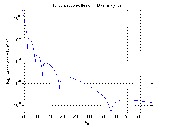
Figure 2: The absolute value of the relative difference between the analytical and the FD solutions for the convection-diffusion problem as a function of the initial asset value $A_{1,0}$.

In the second test we extend the previous case by adding exponential jumps to the first component. Again, this problem admits an analytical solution which could be expressed via the inverse Laplace transform, see Lipton, 2002a where this problem was solved by using fluctuation identities. It can also be solved by using a generalized transform of Lewis, (2000) combined with the Wiener-Hopf method, see, e.g., Kuznetsov et al., (2011). The corresponding solution reads

$$Q=1-\mathcal{L}_{q}^{-1}\left\{\frac{\displaystyle e^{\beta\hat{\rho}_{1}(q)}}{\displaystyle q}\right\}.$$

Here $\hat{\rho}_{1}$ is the only negative root of the characteristic equation in the Wiener-Hopf method, $\beta=\log(B_{a}/a_{0})<0$, and $B_{a}$ is the default boundary.

Also within the framework of Itkin, 2014c which we use in this paper, exponential jumps were never considered. Therefore, in Appendix C for completeness, we construct a finite-difference algorithm for exponential jumps.

In Fig. 3 the absolute value of the relative difference between the analytical and numerical solutions is depicted as a function of $A_{1,0}$. In this experiment we set the intensity of the jumps $\lambda=0.7$, and the parameter of the exponential distribution $\phi=2$.

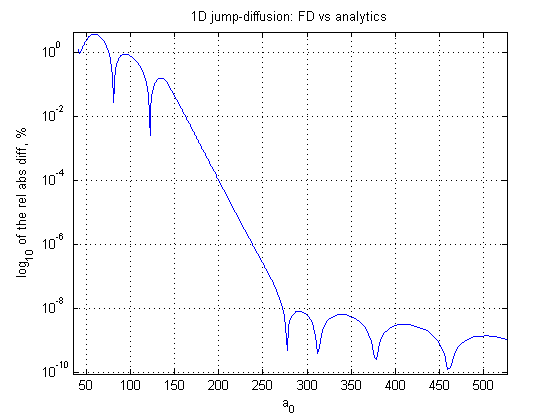
Figure 3: The absolute value of the relative difference between the analytical and the FD solutions for the jump-diffusion problem as a function of the initial asset value $A_{1,0}$.

The difference is less than 1% except close to the barrier; see also Table 2.

$A_{1,0}$	$Q_{an}$	$Q_{FD}$	$\Delta Q$
40.85	0.008805	0.008909	-0.000103
41.69	0.017710	0.017874	-0.000164
42.53	0.026710	0.026972	-0.000262
43.36	0.035802	0.036188	-0.000387
44.18	0.044982	0.045523	-0.000541
44.99	0.054251	0.054981	-0.000729
45.79	0.063610	0.064563	-0.000953
46.59	0.073058	0.074273	-0.001215
47.38	0.082601	0.084116	-0.001515
48.16	0.092241	0.094094	-0.001853
48.94	0.101984	0.104212	-0.002228
49.70	0.111833	0.114472	-0.002639
50.46	0.121795	0.124878	-0.003083
51.22	0.131876	0.135431	-0.003556
51.96	0.142080	0.146134	-0.004054
52.70	0.152413	0.156985	-0.004571
53.43	0.162881	0.167985	-0.005104
54.16	0.173486	0.179132	-0.005646
54.88	0.184233	0.190423	-0.006190
55.60	0.195123	0.201854	-0.006732

Table 2: Results for the 1D jump-diffusion test: $Q_{an},Q_{FD}$ - the analytical and numerical survival probabilities, $\Delta Q=Q_{anal}-Q_{FD}$.

7.2 The two-dimensional problem

In the first test we solve Eq.(9) with parameters of the model given in Table 3.

$A_{1,0}$	$A_{2,0}$	$L_{1,0}$	$L_{2,0}$	$L_{12,0}$	$L_{21,0}$	$R_{1}$	$R_{2}$	$r$	T	$\sigma_{1}$	$\sigma_{2}$	$\rho$
110	100	80	85	10	15	0.4	0.35	0.05	1	0.2	0.3	0.5

Table 3: Parameters of the structural default model.

For idiosyncratic jumps we chose the Merton model with parameters ($\varphi^{i},\mu^{i}_{M},\sigma^{i}_{M}),i=1,2$, and for systemic jumps we chose the Kou model with parameters $\varphi_{12},p,\theta_{1},\theta_{2}$, as shown in Table 4. We use the upper script ⁽ⁱ⁾ to mark the $i$th bank. Also in these experiments without loss of generality we use $\varphi_{1}=\varphi_{2}=\varphi_{12}\equiv\varphi$.

We computed all tests using a $100\times 100$ spatial grid for the convection-diffusion problem. Also we use a constant step in time $\Delta\tau=0.01$, so that the total number of time steps for a given maturity is also 100. The non-uniform grid for jumps in each direction is a superset of the convection-diffusion grid up to $A_{i}=10^{5}$. It is built using a geometric progression and contains 80 nodes.

$\varphi$	$\mu_{M}^{(1)}$	$\mu_{M}^{(2)}$	$\sigma_{M}^{(1)}$	$\sigma_{M}^{(2)}$	$p$	$\theta_{1}$	$\theta_{2}$	$b_{1}$	$b_{2}$
3	0.5	0.3	0.3	0.4	0.3445	3.0465	3.0775	0.2	0.3

Table 4: Parameters of the jump models.

In Fig. 4 the joint survival probability $Q(x_{1},x_{2},t,T)$ as computed in our experiment is presented at $t=0$.

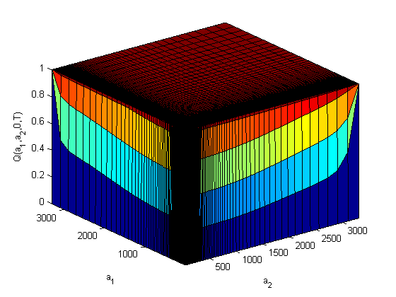
Figure 4: The joint survival probability $Q(x_{1},x_{2},0,T)$.

To better see the behavior of the graph close to the initial values of $A_{1},A_{2}$ we zoom-in this picture in the vicinity of these values, see Fig. 5.

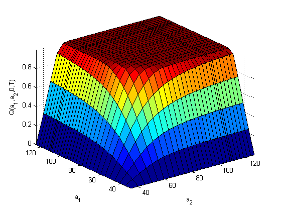
Figure 5: The joint survival probability $Q(x_{1},x_{2},0,T)$, a zoomed-in picture.

We compare these survival probabilities with those obtained when two banks don’t have mutual liabilities. The difference in the corresponding probabilities is shown in Fig. 6.

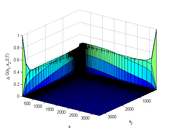
Figure 6: The difference $\Delta Q$ between the joint survival probabilities with and without mutual liabilities.

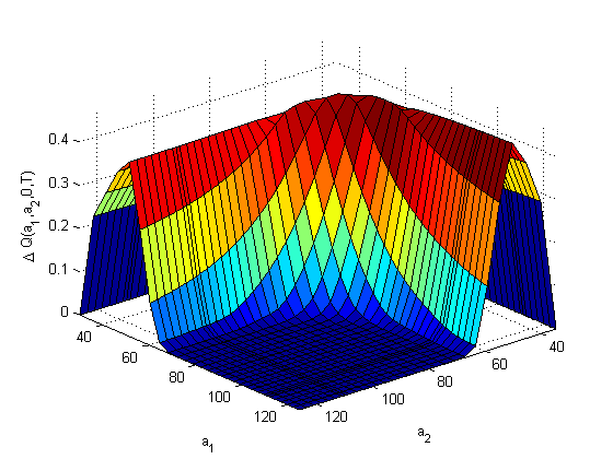
Figure 7: The difference $\Delta Q$, a zoomed-in picture.

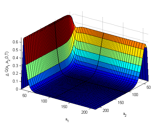
Figure 8: The difference $\Delta Q$ for the pure diffusion case (the picture is rotated by 180^∘).

As expected the maximal difference occurs near default boundaries where the difference could be of order 1. To see how pronounced this effect is, see Fig. 7. Obviously, the magnitude depends on the values of the jump parameters used in the test as well as on the other parameters of the model and the default boundaries. Also, the effect becomes more pronounced when the ratio of the mutual liabilities to the other liabilities increases.

To emphasize the role of jumps, the same test was conducted without jumps in a pure diffusion setting. The results are shown in Fig. 8. Clearly, the presence of jumps significantly changes the picture, while still preserving the effect of mutual liabilities.

In the second set of tests we setup a local volatility function for assets 1 and 2, which is given in Tables 5, 6

$t,\mbox{yrs}$	$A_{1,0}$
	70	80	90	100	110	120	130	140	150
0.1	0.447	0.455	0.459	0.462	0.465	0.467	0.468	0.470	0.471
0.2	0.500	0.507	0.511	0.514	0.516	0.518	0.519	0.520	0.522
0.4	0.548	0.554	0.558	0.560	0.562	0.564	0.565	0.566	0.567
0.6	0.592	0.597	0.601	0.603	0.605	0.607	0.608	0.609	0.610
0.8	0.632	0.638	0.641	0.643	0.645	0.646	0.648	0.649	0.650

Table 5: Local volatility function for $A_{1,t}$.

$t,\mbox{yrs}$	$A_{2,0}$
	50	60	70	80	90	100	110	120	130	140
0.1	0.548	0.554	0.558	0.560	0.562	0.564	0.565	0.566	0.567	0.568
0.2	0.592	0.597	0.601	0.603	0.605	0.607	0.608	0.609	0.610	0.611
0.4	0.632	0.638	0.641	0.643	0.645	0.646	0.648	0.649	0.650	0.650
0.6	0.671	0.676	0.679	0.681	0.683	0.684	0.685	0.686	0.687	0.688
0.8	0.707	0.712	0.715	0.719	0.718	0.720	0.721	0.722	0.722	0.723

Table 6: Local volatility function for $A_{2,t}$.

The results of this test are given in Fig. 9. It can be seen that larger volatilities amplify the effect of mutual liabilities, as well as make a shape of $Q$ highly asymmetric.

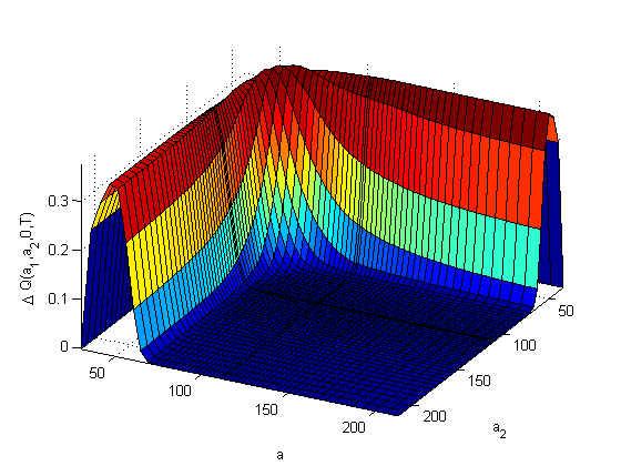
Figure 9: The difference $\Delta Q$ in the presence of local volatility.

We also consider a case of long maturity, $T=10$ years to investigate how the time horizon affects the shape of the joint survival probability $Q(x_{1},x_{2},0,T)$ in the presence of mutual liabilities. The corresponding results are shown in Fig. 10, Fig. 11. It is clear that the effect of mutual liabilities significantly decreases when $T$ increases. That is because $Q(x_{1},x_{2},0,T)$ itself decreases in absolute value with larger $T$, and therefore the absolute value of the effect also drops down.

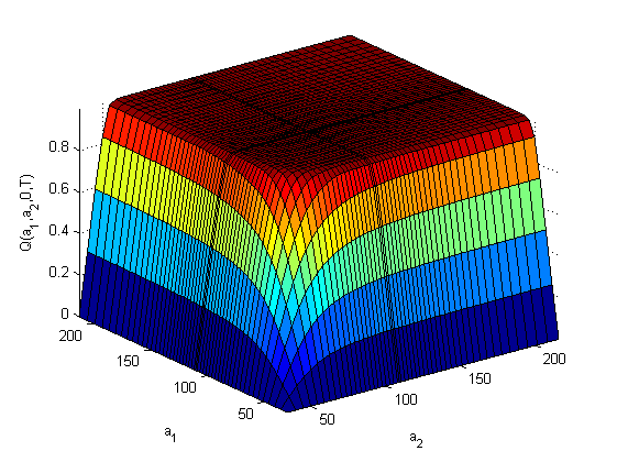
Figure 10: The joint survival probability $Q(a_{1},a_{2},0,T)$ at $T=10$ years

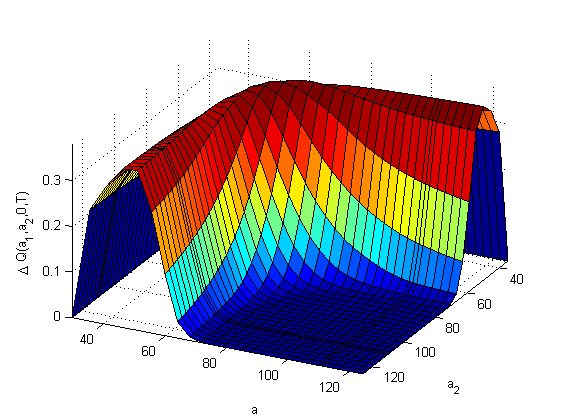
Figure 11: The difference $\Delta Q$ at $T=10$ years with local volatility.

The following tests show the influence of correlations on the effects caused by mutual liabilities. In Fig. 12 the same results as in Test 1 are presented when $\rho=0$, while in Fig. 13 we assume that $b_{1}=b_{2}=0$.

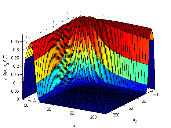
Figure 12: The difference $\Delta Q$ with local volatility and $\rho_{12}=0$.

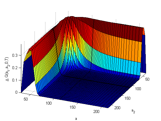
Figure 13: The difference $\Delta Q$ with local volatility and $b_{1}=b_{2}=0$.

These figures show that both contributions of correlations are important.

Fig. 14 represents the marginal survival probability of the first bank as a function of the initial asset value of the second bank under the conditions of the first test in Fig. 4. And Fig. 15 shows the difference in marginal survival probabilities with and without mutual interbank liabilities.

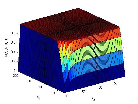
Figure 14: The marginal survival probability $q(x_{1},0,T|x_{2})$, a zoomed-in picture.

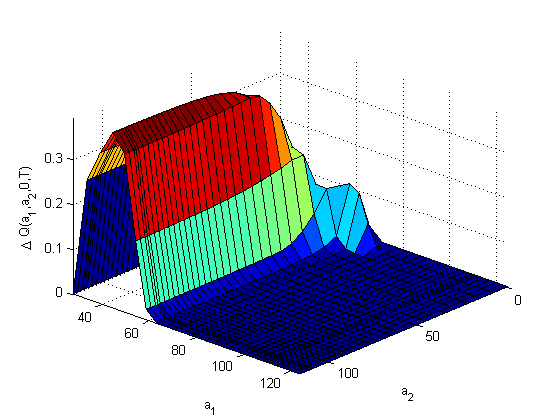
Figure 15: The difference in the marginal survival probabilities $\Delta q(x_{1},0,T|x_{2})$.

As could be seen mutual interbank liabilities affect both the marginals and joint survival probabilities. The influence on marginals despite being smaller in magnitude, is still significant.

8 The three-dimensional case

It is more natural to consider at least three banks, $A_{i},\ i=1,2,3$ using the same structural default model as above. Also assume that all three banks have mutual liabilities to each other, as well as liabilities with respect to the outside economy. The advantage of our approach lies in the fact that just minor changes in the computational algorithm need to be done to include the third asset into the whole picture.

Since now $Q=Q(x_{1},x_{2},x_{3},t,T)$, we need to replace the two-dimensional matrices with the three-dimensional ones. Therefore, the expected complexity of the method becomes $O(N_{1}N_{2}N_{3})$. As idiosyncratic jumps are still independent, our splitting algorithm remains the same, although we need to add two more steps in the direction $x_{3}$ to Eq.(21). Hence, the 3D splitting algorithm reads

$$Q^{(1)}(x_{1},x_{2},x_{3},\tau) = e^{\frac{\Delta\tau}{2}\mathcal{D}}Q(x_{1},x_{2},x_{3},\tau),$$ (32)

$$Q^{(2)}(x_{1},x_{2},x_{3},\tau) = e^{\frac{\Delta\tau}{2}\mathcal{J}_{1}}Q^{(1)}(x_{1},x_{2},x_{3},\tau),$$

$$Q^{(3)}(x_{1},x_{2},x_{3},\tau) = e^{\frac{\Delta\tau}{2}\mathcal{J}_{2}}Q^{(2)}(x_{1},x_{2},x_{3},\tau),$$

$$Q^{(4)}(x_{1},x_{2},x_{3},\tau) = e^{\frac{\Delta\tau}{2}\mathcal{J}_{3}}Q^{(3)}(x_{1},x_{2},x_{3},\tau),$$

$$Q^{(5)}(x_{1},x_{2},x_{3},\tau) = e^{\Delta\tau\mathcal{J}_{12}}Q^{(4)}(x_{1},x_{2},x_{3},\tau),$$

$$Q^{(6)}(x_{1},x_{2},x_{3},\tau) = e^{\frac{\Delta\tau}{2}\mathcal{J}_{3}}Q^{(5)}(x_{1},x_{2},x_{3},\tau),$$

$$Q^{(7)}(x_{1},x_{2},x_{3},\tau) = e^{\frac{\Delta\tau}{2}\mathcal{J}_{2}}Q^{(6)}(x_{1},x_{2},x_{3},\tau),$$

$$Q^{(8)}(x_{1},x_{2},x_{3},\tau) = e^{\frac{\Delta\tau}{2}\mathcal{J}_{1}}Q^{(7)}(x_{1},x_{2},x_{3},\tau),$$

$$Q(x_{1},x_{2},x_{3},\tau+\Delta\tau) = e^{\frac{\Delta\tau}{2}\mathcal{D}}Q^{(8)}(x_{1},x_{2},x_{3},\tau).$$

In our test experiments at step 5, without loss of generality, we again use the Kou model for the systemic jumps. That requires solving the corresponding 3D linear equations of the first order similar to Eq.(26) and Eq.(29). The solution could be constructed by using a 3D version of the ADI scheme derived in a similar manner to the 2D case (McDonough, (2008)). For the sake of brevity, we formulate two propositions and give just a sketch of the proof since it could be obtained in exactly the same way as in Appendices.

Proposition 8.1

Consider the following PIDE

$$(\theta_{1}-b_{1}\triangledown_{x_{1}}-b_{2}\triangledown_{x_{2}}-b_{3}\triangledown_{x_{3}})z(x_{1},x_{2},\tau)=p\theta_{1}Q(x_{1},x_{2},x_{3},\tau).$$ (33)

and solve it using the following ADI scheme

$$\Big{[}\Big{(}s +\frac{\displaystyle 1}{\displaystyle 2}\theta_{1}\Big{)}-b_{1}\triangledown_{x_{1}}\Big{]}z^{*}({\bf x},\tau)=\Big{[}\Big{(}s-\frac{\displaystyle 1}{\displaystyle 2}\theta_{1}\Big{)}+b_{2}\triangledown_{x_{2}}+b_{3}\triangledown_{x_{3}}\Big{]}z^{k}({\bf x},\tau)+b$$

$$\Big{[}\Big{(}s +\frac{\displaystyle 1}{\displaystyle 2}\theta_{1}\Big{)}-b_{2}\triangledown_{x_{2}}\Big{]}z^{**}({\bf x},\tau)=\Big{[}\Big{(}s-\frac{\displaystyle 1}{\displaystyle 2}\theta_{1}\Big{)}+b_{1}\triangledown_{x_{1}}+b_{3}\triangledown_{x_{3}}\Big{]}z^{*}({\bf x},\tau)+b$$

$$\Big{[}\Big{(}s +\frac{\displaystyle 1}{\displaystyle 2}\theta_{1}\Big{)}-b_{3}\triangledown_{x_{3}}\Big{]}z^{k+1}({\bf x},\tau)=\Big{[}\Big{(}s-\frac{\displaystyle 1}{\displaystyle 2}\theta_{1}\Big{)}+b_{1}\triangledown_{x_{1}}+b_{2}\triangledown_{x_{2}}\Big{]}z^{**}({\bf x},\tau)+b$$

$$b \equiv p\theta_{1}Q(x_{1},x_{2},x_{3},\tau)$$

Then the discrete approximation of this ADI scheme

$$\Big{[}\Big{(}s +\frac{\displaystyle 1}{\displaystyle 2}\theta_{1}\Big{)}I_{x_{1}}-b_{1}A(x_{1})\Big{]}z^{*}({\bf x},\tau)=\Big{[}\Big{(}s-\frac{\displaystyle 1}{\displaystyle 2}\theta_{1}\Big{)}I_{x_{2}}+b_{2}A(x_{2})+b_{3}A(x_{3})\Big{]}z^{k}({\bf x},\tau)+b$$

$$\Big{[}\Big{(}s +\frac{\displaystyle 1}{\displaystyle 2}\theta_{1}\Big{)}I_{x_{2}}-b_{2}A(x_{2})\Big{]}z^{**}({\bf x},\tau)=\Big{[}\Big{(}s-\frac{\displaystyle 1}{\displaystyle 2}\theta_{1}\Big{)}I_{x_{1}}+b_{1}A(x_{1})+b_{3}A(x_{3})\Big{]}z^{*}({\bf x},\tau)+b$$

$$\Big{[}\Big{(}s +\frac{\displaystyle 1}{\displaystyle 2}\theta_{1}\Big{)}I_{x_{3}}-b_{3}A(x_{3})\Big{]}z^{k+1}({\bf x},\tau)=\Big{[}\Big{(}s-\frac{\displaystyle 1}{\displaystyle 2}\theta_{1}\Big{)}I_{x_{1}}+b_{1}A(x_{1})+b_{2}A(x_{2})\Big{]}z^{**}({\bf x},\tau)+b$$

$$b \equiv p\theta_{1}Q(x_{1},x_{2},x_{3},\tau),\qquad A(x_{i})=\begin{cases}A_{2}^{F}(x_{i}),&b_{i}>0\\ A_{2}^{B}(x_{i}),&b_{i}<0,\qquad i=1,2\end{cases}$$

is unconditionally stable, approximates Eq.(33) with $O\left(\sum_{i,j=1}^{3}\Delta x_{i}\Delta x_{j}\right)$ and preserves positivity of the solution.

• The proof could be obtained following the lines of Proof of Proposition 6.1 given in Appendix A. In our situation we apply the same discretization three times (to each row of the splitting scheme). The remaining part of the proof is exactly same as in Appendix A.

The second proposition is similar in nature.

Proposition 8.2

Consider the following PIDE

$$(\theta_{2}+b_{1}\triangledown_{x_{1}}+b_{2}\triangledown_{x_{2}}+b_{3}\triangledown_{x_{3}})z(x_{1},x_{2},\tau)=(1-p)\theta_{2}Q(x_{1},x_{2},x_{3},\tau).$$ (34)

and solve it using the following ADI scheme

$$\Big{[}\Big{(}s +\frac{\displaystyle 1}{\displaystyle 2}\theta_{2}\Big{)}+b_{1}\triangledown_{x_{1}}\Big{]}z^{*}(x_{1},x_{2},\tau)=\Big{[}\Big{(}s-\frac{\displaystyle 1}{\displaystyle 2}\theta_{2}\Big{)}-b_{2}\triangledown_{x_{2}}-b_{3}\triangledown_{x_{3}}\Big{]}z^{k}(x_{1},x_{2},\tau)+b$$

$$\Big{[}\Big{(}s +\frac{\displaystyle 1}{\displaystyle 2}\theta_{2}\Big{)}+b_{2}\triangledown_{x_{2}}\Big{]}z^{**}(x_{1},x_{2},\tau)=\Big{[}\Big{(}s-\frac{\displaystyle 1}{\displaystyle 2}\theta_{2}\Big{)}-b_{1}\triangledown_{x_{2}}-b_{3}\triangledown_{x_{3}}\Big{]}z^{*}(x_{1},x_{2},\tau)+b$$

$$\Big{[}\Big{(}s +\frac{\displaystyle 1}{\displaystyle 2}\theta_{2}\Big{)}+b_{3}\triangledown_{x_{3}}\Big{]}z^{k+1}(x_{1},x_{2},\tau)=\Big{[}\Big{(}s-\frac{\displaystyle 1}{\displaystyle 2}\theta_{2}\Big{)}-b_{1}\triangledown_{x_{1}}-b_{2}\triangledown_{x_{2}}\Big{]}z^{**}(x_{1},x_{2},\tau)+b$$

$$b \equiv(1-p)\theta_{2}Q(x_{1},x_{2},x_{3},\tau)$$

Then the discrete approximation of this ADI scheme

$$\Big{[}\Big{(}s +\frac{\displaystyle 1}{\displaystyle 2}\theta_{2}\Big{)}I_{x_{1}}+b_{1}A(x_{1})\Big{]}z^{*}(x_{1},x_{2},\tau)=\Big{[}\Big{(}s-\frac{\displaystyle 1}{\displaystyle 2}\theta_{2}\Big{)}I_{x_{2}}-b_{2}A(x_{2})-b_{3}A(x_{3})\Big{]}z^{k}(x_{1},x_{2},\tau)+b$$

$$\Big{[}\Big{(}s +\frac{\displaystyle 1}{\displaystyle 2}\theta_{2}\Big{)}I_{x_{2}}+b_{2}A(x_{2})\Big{]}z^{**}(x_{1},x_{2},\tau)=\Big{[}\Big{(}s-\frac{\displaystyle 1}{\displaystyle 2}\theta_{2}\Big{)}I_{x_{1}}-b_{1}A(x_{1})-b_{3}A(x_{3})\Big{]}z^{*}(x_{1},x_{2},\tau)+b$$

$$\Big{[}\Big{(}s +\frac{\displaystyle 1}{\displaystyle 2}\theta_{2}\Big{)}I_{x_{3}}+b_{3}A(x_{3})\Big{]}z^{k+1}(x_{1},x_{2},\tau)=\Big{[}\Big{(}s-\frac{\displaystyle 1}{\displaystyle 2}\theta_{2}\Big{)}I_{x_{1}}-b_{1}A(x_{1})-b_{2}A(x_{2})\Big{]}z^{**}(x_{1},x_{2},\tau)+b$$

$$b \equiv(1-p)\theta_{2}Q(x_{1},x_{2},x_{3},\tau),\qquad A(x_{i})=\begin{cases}A_{2}^{B}(x_{i}),&b_{i}>0\\ A_{2}^{F}(x_{i}),&b_{i}<0,\qquad i=1,2\end{cases}$$

is unconditionally stable, approximates Eq.(34) with $O\left(\sum_{i,j=1}^{3}\Delta x_{i}\Delta x_{j}\right)$ and preserves positivity of the solution.

• The proof is analogous to that given in Appendix B if one applies the same discretization three times (to each row of the splitting scheme). The remaining part of the proof is exactly the same as in Appendix B, which in turn is analogous to Appendix A.

The solution of the 3D convection-diffusion problem at the first and the last steps of the scheme is more challenging. So far the unconditional stability of some schemes (Craig-Sneid, Modified Craig-Sneid (MCS), Hundsdorfer-Verwer (HV), etc.) was proven only when there is no drift term in the corresponding diffusion equation (In’t Hout and Mishra, (2013)). Therefore, this problem requires further attention. Nevertheless, these schemes were successfully used in the 3D setup by Haentjens and In’t Hout, (2012) where the MCS and HV schemes demonstrated good stability if the scheme parameter $\theta$ was chosen similar to In’t Hout and Mishra, (2013).

8.1 Numerical experiments

In our tests we chose parameters of the model similar to the 2D case, see Tables 7, 8

$A_{1,0}$	$A_{2,0}$	$A_{3,0}$	$L_{1,0}$	$L_{2,0}$	$L_{3,0}$	$r$	$T$	$\rho_{xz}$	$\rho_{yz}$
110	100	120	80	90	100	0.05	1	0.5	0.3
$\phi_{xy}$	$L_{12,0}$	$L_{21,0}$	$L_{13,0}$	$L_{31,0}$	$L_{23,0}$	$L_{32,0}$	$R_{1}$	$R_{2}$	$R_{3}$
$2\pi/5$	20	15	15	20	10	15	0.4	0.35	0.5

Table 7: Parameters of the 3D structural default model.

$\varphi$	$\mu_{M}^{(1)}$	$\mu_{M}^{(2)}$	$\mu_{M}^{(3)}$	$\sigma_{M}^{(1)}$	$\sigma_{M}^{(2)}$	$\sigma_{M}^{(3)}$	$p$	$\theta_{1}$	$\theta_{2}$	$b_{1}$	$b_{2}$	$b_{3}$
3	0.5	0.3	0.4	0.3	0.4	0.5	0.3445	3.0465	3.0775	0.2	0.3	0.25

Table 8: Parameters of the 3D jump models.

We recall that a correlation matrix $\Sigma$ of $N$ assets can be represented as a Gram matrix with matrix elements $\Sigma_{ij}=\left<{\bf x}_{i},{\bf x}_{j}\right>$ where ${\bf x}_{i},{\bf x}_{j}$ are unit vectors on a $N-1$ dimensional hyper-sphere $\mathbb{S}^{N-1}$. Using the 3D geometry, it is easy to establish the following cosine law for the correlations between three assets:

$$\rho_{xy}=\rho_{yz}\rho_{xz}+\sqrt{(1-\rho_{yz}^{2})(1-\rho_{xz}^{2})}cos(\phi_{xy})$$

with $\phi_{xy}$ being an angle between $\bf x$ and its projection on the plane spanned by ${\bf y},{\bf z}$. As discussed, e.g., by Dash, (2004), three variables $\rho_{yz},\rho_{zz},\phi_{xy}$ are independent, but $\rho_{xy},\rho_{xz},\rho_{yz}$ are not. Based on the values given in Tab. 7 we find $\rho_{xy}=0.4053$.

We compute the test using a $50\times 50\times 50$ spatial grid for the convection-diffusion problem. Also we use a constant time step $\Delta\tau=0.025$, so that the total number of time steps for the given maturity is 40. The jump non-uniform grid in each direction is a superset of the convection-diffusion grid up to $A_{i}=10^{4}$ built using a geometric progression. So the jumps are computed on the grid with $62\times 64\times 63$ nodes. Also we chose $s_{i}=\theta_{i}+1,\ i\in[1,3]$ which provided convergence of the ADI scheme for the common jumps after 4 iterations.

We again compare the survival probability in the presence of mutual liabilities, $Q^{w}(A_{1},A_{2}$, $A_{3})$, with that in the absence of mutual liabilities, $Q^{wo}(A_{1},A_{2},A_{3})$. To obtain the latter, we first reduce $L_{1,0},L_{2,0},L_{3,0}$ by the amounts $L_{ij,0},\ i\in[1,3],\ j\in[1,3],i\neq j$, and then put $L_{ij,t}=0$. The difference $\Delta Q=Q^{w}-Q^{wo}$ is presented in Fig. 16 - 18. Since the whole picture in this case is four-dimensional, we represent it as a series of 3D projections, namely: Fig. 16 represents the $A_{1}-A_{2}$ plane at various values of the $A_{3}$ coordinate which are indicated in the corresponding labels; Fig. 17 does same in the $A_{1}-A_{3}$ plane, and Fig. 18 - in the $A_{2}-A_{3}$ plane.

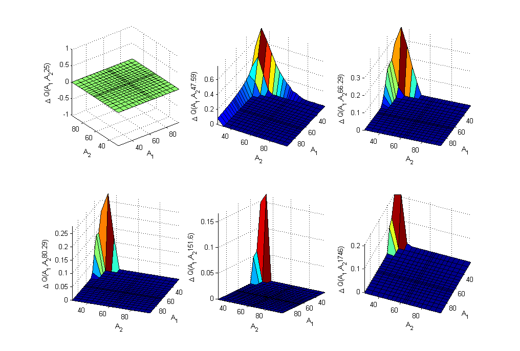
Figure 16: The difference $\Delta Q$ with and without mutual liabilities, $A_{1}-A_{2}$ plane.

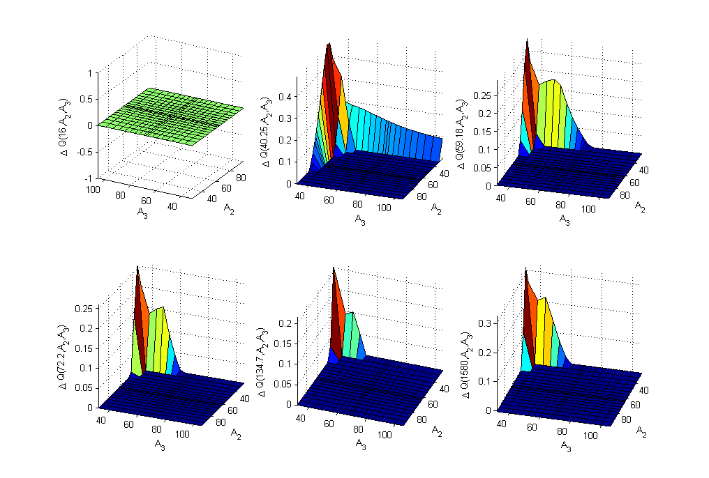
Figure 17: The difference $\Delta Q$ with and without mutual liabilities, $A_{1}-A_{3}$ plane.

Figure 18: The difference $\Delta Q$ with and without mutual liabilities, $A_{2}-A_{3}$ plane.

Two observations could be made based on the results obtained in these tests. First, when three banks have mutual liabilities, their effect on the joint survival probability is more profound than in the 2D case. Second, $\Delta Q$ has an irregular shape as a function of 3 coordinates. For instance, in the $A_{2}-A_{3}$ plane it has two local maxima (in the absolute value) while in the 2D case it doesn’t demonstrate such a behavior. Also this effect disappears in the absence of jumps. This is similar to the effect observed in Itkin and Carr, (2011) where asymmetric positive and negative jumps in the stochastic skew model were described by the CGMY model with different $\alpha$, which produced a qualitatively new effect. It is evident through the appearance of a big dome close to the ATM at the moderate values of the instantaneous variance $v$ in addition to a standard arc of the double barrier options which is also close to the ATM, but at small values of $v$.

As expected, the whole picture is rather complicated. Moreover, as it is affected by the number of model parameters, which could be difficult to extract from a set of liquid market data, it could be very challenging to calibrate such a model. A standard recipe is to first calibrate marginals of the distribution to the corresponding market data, and then use some other data for calibration of the remaining parameters.

9 Conclusions

In this paper we presented three main innovations which seem to be rather general, namely:

1. We introduced mutual banks’ liabilities into the structural default model. We discussed how these liabilities affect joint and marginal survival probabilities, and provided some numerical test results. These results demonstrate that the effect of mutual liabilities could be quite significant. Of course, the magnitude of the effect depends on how close the initial asset values are to the default barrier, and parameters which describe the assets’ dynamics, such as volatility, etc. These parameters, in principle, could be found by calibrating marginal survival probabilities to market CDS spreads.

2. To make the above analysis tractable we developed a solution scheme for the model considering a set of banks with mutual interbank liabilities whose assets are driven by correlated Lévy processes. For every asset, the jumps are represented as a weighted sum of the common and idiosyncratic parts. Both parts could be simulated by an arbitrary Lévy model which is an extension of the previous approaches where either the discrete or exponential jumps were considered, or a Lévy copula approach was utilized. We provided a novel efficient (linear complexity in each dimension) numerical (splitting) algorithm for solving the corresponding 2D and 3D jump-diffusion equations, and proved its convergence and second order of accuracy in both space and time.

3. The joint survival probability of three firms $Q(x_{1},x_{2},x_{3},0,T)$ was computed using the above framework. To the best of our knowledge there were no the similar results reported in literature. We found that in some cases, the difference between the joint survival probabilities with and without mutual liabilities has a bimodal profile in some projections, and this effect disappears in the pure diffusion setup. This is similar to what was observed in Itkin and Carr, (2011) where interaction of jumps also produced a bimodal distribution for double barrier option prices.

Despite the fact that the present approach is efficient and attractive in low dimensions, it is not clear how best to extend it to the case when the number of firms is more than three, unless some simplifications are introduced into the model. This is a standard limitation of the FD approach which experiences the curse of dimensionality. A possible way to overcome this could be to combine the analytical and numerical methods, similar to how this was done in, e.g., Lipton and Savescu, (2014).

Appendix A Proof of Proposition 6.1

Following Elhashash and Szyld, (2008), we introduce definition of an EM-matrix

• An $N\times N$ matrix $A=[a_{ij}]$ is called an EM-Matrix if it can be represented as $A=sI-B$ with $0<\rho(B)<s$, $s>0$ is some constant, $\rho(B)$ is the spectral radius of $B$, and $B$ is an eventually nonnegative matrix.

Now suppose $b_{1}<0,\ b_{2}<0$. Then the matrix

$$M_{1}=\Big{[}\Big{(}s+\frac{\displaystyle 1}{\displaystyle 2}\theta_{1}\Big{)}I_{x_{1}}-b_{1}A^{B}_{2}(x_{1})\Big{]}$$

in the first row of Eq.(28) is an EM-matrix, see Lemma A.2 in Itkin, 2014c . Therefore, the inverse of $M_{1}$ is a non-negative matrix, see Lemma A.3 in Itkin, 2014c .

The matrix

$$M_{2}=\Big{[}\Big{(}s-\frac{\displaystyle 1}{\displaystyle 2}\theta_{1}\Big{)}I_{x_{2}}+b_{2}A_{2}^{B}(x_{2})\Big{]}$$

is an eventually non-negative matrix if $s$ is chosen to provide

$$s>\frac{\displaystyle 1}{\displaystyle 2}\theta_{1}-b_{2}\frac{\displaystyle 3}{\displaystyle h}$$ (35)

Therefore, the solution of the first row of Eq.(28) is $z^{*}(x_{1},x_{2},\tau)=M_{1}^{-1}\left[M_{2}z^{k}(x_{1},x_{2},\tau)+b\right]$ which by construction is a non-negative vector. Also eigenvalues of $M_{1}^{-1}M_{2}$ are

$$\lambda_{i}=\frac{\displaystyle s-\frac{\displaystyle 1}{\displaystyle 2}\theta_{1}+3b_{2}/h}{\displaystyle s+\frac{\displaystyle 1}{\displaystyle 2}\theta_{1}-3b_{1}/h}<1,\qquad i\in[1,N_{1}]$$

Therefore, this scheme converges unconditionally provided Eq.(35) is satisfied.

Also, by construction the matrix $A_{2}^{B}(x)$ approximates the operator $\triangledown_{x}$ to the second order, i.e., with $O(h^{2})$. Therefore, the whole scheme provides the second order approximation.

The second row of Eq.(28) could be analyzed in the same way.

In all other cases $b_{1}<0,b_{2}>0$, $b_{1}>0,b_{2}<0$ and $b_{1}>0,b_{2}>0$ the proof could be done by analogy.

Appendix B Proof of Proposition 6.2

The proof is completely analogous to that in Appendix A.

Appendix C Matrix exponential approach for exponential jumps

In the 1D case we still want to use the splitting algorithm of Eq.(19). To proceed, let us define an explicit model for jumps, so the pseudo-differential operator $\mathcal{J}$ defined in Eq.(14) could be computed explicitly.

Let us consider only negative exponentially distributed jumps, see Lipton, 2002a , i.e.

$$\nu(J)=\begin{cases}\phi e^{\phi J},&J\leq 0\cr 0,&J>0,\end{cases}$$ (36)

where $\phi>0$ is the parameter of the exponential distribution. With the Lévy measure $\nu(dy)$ given in Eq.(36) and the intensity of jumps $\lambda\geq 0$ we can substitute $\nu(dy)$ into Eq.(14) and integrate. The result reads

$$\mathcal{J}=\frac{\displaystyle\lambda}{\displaystyle\phi+1}(\phi+\triangledown_{x})^{-1}(\triangledown_{x}^{2}-\triangledown_{x}),\qquad\triangledown_{x}\equiv\partial_{x}.$$ (37)

Below for simplicity of notation we introduce $a\equiv A_{1}$. Since $x=\log a$, the above expression could be re-written as

$$\mathcal{J}=\frac{\displaystyle\lambda}{\displaystyle\phi+1}(\phi+a\triangledown)^{-1}a^{2}\triangledown^{2},\qquad\triangledown\equiv\partial_{a}.$$ (38)

Proposition C.1

Consider the following discrete approximation of Eq.(38):

$$J=\frac{\displaystyle\lambda}{\displaystyle\phi+1}(\phi I+aA^{B}_{2})^{-1}a^{2}A^{C}_{2}.$$ (39)

Then this scheme is a) unconditionally stable; b) approximates the operator $\mathcal{J}$ in Eq.(38) on a certain non-uniform grid in variable $a$ with $O(\max(h_{i})^{2})$, where $h_{i},\ i=1,...,N$ are the steps of the grid; c) and preserves positivity of the solution.

• For the sake of clarity we give the proof for the uniform grid, as an extension to the non-uniform grid is straightforward.

  As shown in Itkin, 2014c the matrix $A^{B}_{2}$ is an EM matrix. Therefore, the matrix $\phi I+aA^{B}_{2}$ is also an EM-matrix. Therefore, its inverse is a non-negative matrix. The matrix $A^{C}_{2}$ by construction is the Metzler matrix. A product of the non-negative and Metzler matrices is the negative of an EM-matrix. As $\phi>0$, the matrix $J$ is also the negative of an EM-matrix. Then unconditional stability and positivity of the solution follows from the main Theorem in Itkin, 2014c . As the matrix $A^{F}_{2}$ is the second order approximation in $h$ to $\triangledown$, and $A^{C}_{2}$ is the second order approximation in $h$ to $\triangledown^{2}$, the whole scheme approximates the operator $\mathcal{J}$ with the second order in $h$.

In practical applications the complexity of this scheme could be linear in the number of grid nodes $N$. Indeed, suppose we wish to compute $Q$ with the second order of approximation in the time step $\Delta t$, i.e. with the accuracy $O((\Delta t)^{2})$. Represent $e^{\Delta t\lambda J}$ in the second step of the splitting algorithm Eq.(19) using a Padé rational approximation $(1,1)$:

$$e^{\Delta t\lambda J}=\left(I-\frac{\displaystyle 1}{\displaystyle 2}\lambda\Delta tJ\right)^{-1}\left(I+\frac{\displaystyle 1}{\displaystyle 2}\lambda\Delta tJ\right)$$

With allowance for Eq.(39) after some algebra this could be re-written in the form

$$\left[\phi I-aA^{F}_{2}-\frac{\displaystyle\lambda}{\displaystyle 2(\phi-1)}\Delta ta^{2}A^{C}_{2}\right]Q(a,t+\Delta t)=\left[\phi I-aA^{F}_{2}+\frac{\displaystyle\lambda}{\displaystyle 2(\phi-1)}\Delta ta^{2}A^{C}_{2}\right]Q(a,t).$$ (40)

Matrices in square brackets are banded (three or five diagonal), therefore this system of linear equations could be solved with the complexity $O(N)$.

References

- Ballotta and Bonfiglioli, (2014) Ballotta, L. and Bonfiglioli, E. (2014). Multivariate asset models using Lévy processes and applications. SSRN: 1695527.
- Baxter, (2007) Baxter, M. (2007). Lévy simple structural models. International Journal of Theoretical and Applied Finance, 10:607–631.
- Bielecki et al., (2011) Bielecki, T., Crépey, S., and Herbertsson, A. (2011). Markov chain models of portfolio credit risk. In Rennie, A. L. . A., editor, The Oxford Handbook of credit risk, pages 327–382. Oxford University Press.
- Black and Cox, (1976) Black, F. and Cox, J. (1976). Valuing corporate securities: Some effects of bond indenture provisions. Journal of Finance, 31(2):351–367.
- Clift and Forsyth, (2008) Clift, S. and Forsyth, P. (2008). Numerical solution of two asset jump difusion models for option valuation. Appied Numerical Mathematics, 58:743–782.
- Cont and Tankov, (2004) Cont, R. and Tankov, P. (2004). Financial modelling with jump processes. Financial Matematics Series, Chapman & Hall /CRCl.
- Dash, (2004) Dash, J. (2004). Quantitative finance and risk management: a physicist’s approach. World Scientific.
- de Lange and Raab, (1992) de Lange, O. L. and Raab, R. E. (1992). Operator Methods in Quantum Mechanics. Oxford science publications. Chapter 3.
- Deelstra and Petkovic, (2010) Deelstra, G. and Petkovic, A. (2009-2010). How they can jump together: Multivariate Lévy processes and option pricing. Belgian Actuarial Bulletin, 9(1):29–42.
- d’Halluin et al., (2005) d’Halluin, Y., Forsyth, P. A., and Vetzal, K. R. (2005). Robust numerical methods for contingent claims under jump diffusion processes. IMA J. Numerical Analysi, 25:87–112.
- Eberlein, (2009) Eberlein, E. (2009). Jump-type Lévy processes. In Andersen, T. G., Davis, R. A., Kreiß, J.-P., and Mikosch, T., editors, Handbook of Financial Time Series, pages 439–455. Springer Verlag.
- Eberlein and Keller, (1995) Eberlein, E. and Keller, U. (1995). Hyperbolic distributions in finance. Bernoulli, 1:281–299.
- Eisenberg and Noe, (2001) Eisenberg, L. and Noe, T. (2001). Systemic risk in financial systems. Management Science, 47(2):236–249.
- Elhashash and Szyld, (2008) Elhashash, A. and Szyld, D. (2008). Generalizations of M-matrices which may not have a nonnegative inverse. Linear Algebra and its Applications, 429:2435–2450.
- Elsinger et al., (2006) Elsinger, H., Lehar, A., and Summer, M. (2006). Using market information for banking system risk assessment. International Journal of Central Banking, 2(1):137–166.
- Garcia et al., (2009) Garcia, J., Goossens, S., Masol, V., and Schoutens, V. (2009). Lévy based correlation. Wilmott Journal, 1(2):95–100.
- Gauthier et al., (2010) Gauthier, G., Lehar, A., and Souissi, M. (2010). Macroprudential regulation and systemic capital requirements. Technical Report 2010-4, Bank of Canada.
- Guillaume, (2013) Guillaume, F. (2013). The VG model for multivariate asset pricing: calibration and extension. Review of Derivatives Research, 16(1):25–52.
- Haentjens and In’t Hout, (2012) Haentjens, T. and In’t Hout, K. J. (2012). Alternating direction implicit finite difference schemes for the Heston–Hull–White partial differential equation. Journal of Computational Finance, 16:83–110.
- Hilber et al., (2013) Hilber, N., Reichmann, O., Winter, C., and Schwab, C. (2013). Computational Methods for Qantitative Finance. Springer.
- Howison, (1995) Howison, S. (1995). Barrier options. Available at https://people.maths.ox.ac.uk/howison/barriers.pdf.
- In’t Hout and Foulon, (2010) In’t Hout, K. J. and Foulon, S. (2010). ADI finite difference schemes for option pricing in the Heston model with correlation. International journal of numerical analysis and modeling, 7(2):303–320.
- In’t Hout and Mishra, (2013) In’t Hout, K. J. and Mishra, C. (2013). Stability of ADI schemes for multidimensional diffusion equations with mixed derivative terms. Applied Numerical Mathematics, 74:83–94.
- In’t Hout and Welfert, (2007) In’t Hout, K. J. and Welfert, B. D. (2007). Stability of ADI schemes applied to convection-diffusion equations with mixed derivative terms. Applied Numerical Mathematics, 57:19–35.
- (25) Itkin, A. (2014a). Efficient solution of backward jump-diffusion PIDEs with splitting and matrix exponentials. Journal of Computational Finance, forthcoming. electronic version is available at http://arxiv.org/abs/1304.3159.
- (26) Itkin, A. (2014b). High-Order Splitting Methods for Forward PDEs and PIDEs. available at http://arxiv.org/abs/1403.1804.
- (27) Itkin, A. (2014c). Splitting and matrix exponential approach for jump-diffusion models with Inverse Normal Gaussian, Hyperbolic and Meixner jumps. Algorithmic Finance, forthcoming. available at http://arxiv.org/abs/1405.6111.
- Itkin and Carr, (2011) Itkin, A. and Carr, P. (2011). Jumps without tears: A new splitting technology for barrier options. International Journal of Numerical Analysis and Modeling, 8(4):667–704.
- Itkin and Carr, (2012) Itkin, A. and Carr, P. (2012). Using pseudo-parabolic and fractional equations for option pricing in jump diffusion models. Computational Economics, 40(1):63–104.
- Kou and Wang, (2004) Kou, S. and Wang, H. (2004). Option pricing under a double exponential jump diffusion model. Management Science, 50(9):1178–1192.
- Kuznetsov et al., (2011) Kuznetsov, A., Kyprianou, A. E., and Pardo, J. C. (2011). Meromorphic Lévy processes and their fluctuation identities. available at http://arxiv.org/pdf/1004.4671.pdf.
- Lewis, (2000) Lewis, A. L. (2000). Option Valuation under Stochastic Volatility. Finance Press, Newport Beach, California, USA.
- (33) Lipton, A. (2002a). Assets with jumps. Risk, pages 149–153.
- (34) Lipton, A. (2002b). The vol smile problem. Risk, pages 61–65.
- Lipton and Savescu, (2014) Lipton, A. and Savescu, I. (2014). Pricing credit default swaps with bilateral value adjustments. Quantitative Finance, 14(1):171–188.
- Lipton and Sepp, (2009) Lipton, A. and Sepp, A. (2009). Credit value adjustment for credit default swaps via the structural default model. The Journal of Credit Risk, 5(2):123–146.
- Lipton and Sepp, (2011) Lipton, A. and Sepp, A. (2011). Credit value adjustment in the extended structural default model. In The Oxford Handbook of Credit Derivatives, pages 406–463. Oxford University.
- Luciano and Semeraro, (2010) Luciano, E. and Semeraro, P. (2010). Multivariate time changes for Lévy asset models: characterization and calibration. Journal of Computational and Applied Mathematics, 233:1937–1953.
- Mai et al., (2014) Mai, J., Scherer, M., and Schulz, T. (2014). Sequential modeling of dependent jump processes. Wilmott Magazine, 70:54–63.
- Marshall and Olkin, (1967) Marshall, A. and Olkin, I. (1967). A multivariate exponential distribution. Journal of the American Statistical Association, 2:84–98.
- McDonough, (2008) McDonough, J. M. (2008). Lectures on computational numerical analysis of partial differential equations. University of Kentucky. available at http://www.engr.uky.edu/~acfd/me690-lctr-nts.pdf.
- Merton, (1974) Merton, R. (1974). On the pricing of corporate debt: The risk structure of interest rates. Journal of Finance, 29:449—470.
- Moosbrucker, (2006) Moosbrucker, T. (2006). Copulas from infinitely divisible distributions: applications to credit value at risk. Technical report, Department of Banking - University of Cologne. Available at http://gloria-mundi.com/Library_Journal_View.asp?Journal_id=7547.
- Roach, (1976) Roach, P. (1976). Computational fluid dynamics. Hermosa Publishers.
- Schoutens, (2001) Schoutens, W. (2001). Meixner processes in finance. Technical report, K.U.Leuven–Eurandom.
- Strang, (1968) Strang, G. (1968). On the construction and comparison of difference schemes. SIAM J. Numerical Analysis, 5:509–517.
- Sun et al., (2011) Sun, Y., Mendoza-Arriaga, R., and Linetsky, V. (2011). Valuation of collateralized debt obligations in a multivariate subordinator model. In Jain, S., Creasey, R. R., Himmelspach, J., White, K. P., and Fu, M., editors, Proceedings of the 2011 Winter Simulation Conference (WSC), pages 3742–3754. IEEE, Phoenix, AZ.
- Vasicek, (1987) Vasicek, O. (1987). Limiting loan loss probability distribution. Technical report, KMV Co.
- Vasicek, (2002) Vasicek, O. (2002). Loan portfolio value. Risk, 15(12):160–162.
- von Petersdorff and Schwab, (2004) von Petersdorff, T. and Schwab, C. (2004). Numerical solution of parabolic equations in high dimensions. Mathematical Modelling and Numerical Analysis, 38(1):93–127.
- Webber and Willison, (2011) Webber, L. and Willison, M. (2011). Systemic capital requirements. Technical Report 436, Bank of England. available at http://papers.ssrn.com/sol3/papers.cfm?abstract_id=1945654.
- Winter, (2009) Winter, C. (2009). Wavelet Galerkin schemes for option pricing in multidimensional Lévy models. PhD thesis, Eidgenössische Technische Hochschule ETH Zürich.
- Yang et al., (2003) Yang, C., Duraiswami, R., Gumerov, N. A., and Davis, L. (2003). Improved Fast Gauss Transform and efficient kernel density estimation. In EEE International Conference on Computer Vision, pages 464–471.
- Yu, (2007) Yu, F. (2007). Correlated defaults in intensity–based models. Mathematical Finance, 17:155–173.
- Zhou, (2001) Zhou, C. (2001). The term structure of credit spreads with jump risk. Journal of Banking and Finance, 25:2015–2040.