Modeling Non-Progressive Phenomena for Influence Propagation

Abstract

Recent work on modeling influence propagation focus on progressive models, i.e., once a node is influenced (active) the node stays in that state and cannot become inactive. However, this assumption is unrealistic in many settings where nodes can transition between active and inactive states. For instance, a user of a social network may stop using an app and become inactive, but again activate when instigated by a friend, or when the app adds a new feature or releases a new version. In this work, we study such non-progressive phenomena and propose an efficient model of influence propagation. Specifically, we model influence propagation as a continuous-time Markov process with 2 states: active and inactive. Such a model is both highly scalable (we evaluated on graphs with over 2 million nodes), 17-20 times faster, and more accurate for estimating the spread of influence, as compared with state-of-the-art progressive models for several applications where nodes may switch states.

1 Introduction

Study of information and influence propagation over social networks has attracted significant research interest over the past decade, driven by applications such as viral marketing [22, 10], social feed ranking [34], contamination detection [24, 29, 1], and spread of innovation [35] to name a few. A prototypical problem that has received wide attention is influence maximization: given a social network along with pairwise influence probabilities between peers, and a number $k$, find $k$ seed nodes such that activating them at start will eventually lead to the largest number of activated nodes in the network in the expected sense. Following the early work of Domingos and Richardson [10] and Kempe et al. [22], there has been a burst of activity in this area (e.g., see [5, 8, 9, 17, 16, 11, 18]). While the majority of previous studies employ propagation models with discrete time, in recent work, continuous time models have been shown to be more accurate at modeling influence propagation phenomena [11, 16, 28]. We refer the reader to the book [7] for a comprehensive survey and a detailed discussion of recent advances in influence maximization.

As discussed in [22], the propagation models can be classified into progressive and non-progressive (NP) models. In progressive models, an inactive node can become active, but once active, a node cannot become inactive. Non-progressive models relax this restriction and allow nodes to repeatedly transition between active and inactive states.

Indeed, an overwhelming majority of studies of information propagation have confined themselves to progressive models. For applications such as buying a product, the progressive assumption makes perfect sense: buying a product is not easily reversible in many cases. On the other hand, there are real applications which are not naturally captured by progressive models. For example, consider a user adopting a mobile app. Over time, its appeal may fade and her usage of the app may decline over time. Her interest in the app may be rejuvenated by a friend telling her about a new cool feature being added to the app at which point, she decides to try the app again and may continue using it once again. Alternatively, whenever a new version of the app is released, the user feels tempted to try it again and may, with some probability, decide to continue using it again. As a second example, it is well known that fashion follows cycles. Choices that are in fashion at the moment may fall out of fashion and may again become fashionable in the future, as it has been recognized that social choices follow cyclic trends [33]. As a third example, there are many applications where users may become active and stay in that state for a period of time before deactivating, such as, adopting a feature on a content sharing site where the feature may be the “like” or “favorite” button for a post, filters (sepia, sketch, outline) for photo editing, or “check-in” to a location or a show. Finally, in epidemiology, it is well known that an infected person may recover from a disease but not necessarily acquire lifelong immunity from the disease, thus being susceptible to the disease. In all the above examples, the phenomena in question are subject to spreading via influence. As we will show with experiments on real datasets in this paper, the use of progressive models for capturing such phenomena leads to considerable error. There is a clear need for a non-progressive model for studying these phenomena.

We next briefly review related work on non-progressive models. A more detailed comparison appears in the next section. In their seminal paper, Kempe et al. [22] propose a non-progressive model and show that it can be reduced to a progressive model by replicating each node for every timestamp in the time horizon under consideration, and connecting each node to its neighbors in the previous timestamp. They show that this reduction preserves equivalence, which implies all techniques developed for progressive models can in principle be applied to non-progressive models. However, replicating a large network for each timestamp over a large time horizon will clearly make this approach impractical for large social networks containing millions of nodes. Thus, this approach is largely of theoretical interest. Fazli et al. [14] study a simple non-progressive model based on deterministic linear threshold, where the threshold is given by strict majority. Their focus is on finding a minimum perfect target set, i.e., a set of seeds of the smallest size which leads to the eventual activation of all network nodes. The goals and approaches are considerably different from those of this paper. In epidemic modeling, the SIRS (Susceptible-Infected-Recovered-Susceptible) model [31, 15] follows the non-progressive paradigm, and explicitly allows for recovered patients to remain susceptible to the disease and become infected again. In the economics literature, there have studies [4, 12, 20] on non-progressive models. A detailed comparison with these and other related works appears in the next section.

Another related area is competitive influence maximization, where competing parties choose seed nodes in order to maximize the adoption of their product or opinion [7]. Non-progressiveness arises naturally from the perspective of any one party involved in the competition. Our focus in this paper is not competition. As illustrated above, there are several example applications where propagation of information or influence happens in a non-progressive manner and it is our goal to model and study them in this paper.

Influence maximization is known to be a computationally hard problem, even over the relatively simpler progressive models. We don’t expect influence maximization to be easier over non-progressive models. We face the challenge, whether we can design approximation algorithms for influence maximization over non-progressive models that scale to large data sets. To this end, we first propose a discrete time non-progressive model called DNP. It will turn out that DNP, while accurate at modeling non-progressive phenomena, does not lead to a scalable solution for estimating influence spread. To mitigate this, we draw inspiration from the recent observations that continuous time models lead to greater accuracy in predicting node activations [11, 16], and we propose a continuous time non-progressive model (CNP), which models the underlying influence propagation as a Markov process. This model can also capture progressive phenomena by appropriately setting the model parameters. We call this variant CNP-Progressive (CP for short). It is interesting to investigate how CP compares with the state-of-the-art progressive continuous time models such as [11, 16].

A second challenge centers on the question, what should the objective be when selecting seeds with respect to non-progressive models. As opposed to maximizing the number of active nodes at some time, as done in progressive models, we argue that it is more appropriate to maximize the expected time during which nodes may have been active.

Finally, while example applications demonstrating the value of and need for non-progressive models exist, to date, no empirical studies have compared non-progressive models with their progressive counterparts with an aim of calibrating their accuracy for explaining propagation phenomena over real data sets. This is partly exacerbated by the fact that real non-progressive data sets are relatively difficult to obtain. Can we establish the value of non-progressive models using any publicly available data sets?

In this paper, we address all the above challenges. Specifically, we make the following contributions.

• We propose a discrete time non-progressive model and implement it without graph replication (Section 3).

• We propose an efficient continuous time non-progressive model (Section 4).

• We define the objective of influence maximization as choosing seeds so as to maximize the total expected activation time of nodes. We show that the objective function of total expected activation time is both monotone and submodular. This implies the classic greedy seed selection algorithm, combined with our direct approach for computing expected total activation time, provides a $(1-1/e)$-approximation to the optimal solution (Section 6).

• Through experiments on synthetic and real datasets, we show that the accuracy of our non-progressive model for estimating expected total activation time is much higher than its progressive counterparts, including the recently proposed continuous time model [11]. Further, we show that our method is more than one order of magnitude faster than an efficient implementation of the DNP model, whose accuracy is comparable to that of CNP. We also show that on datasets that have no deactivations (i.e., progressive setting), our method using CP is 17-20 times faster than the continuous time progressive model of [11] (Section 7).

We start by presenting related work in Section 2, and conclude with a summary of the paper and a discussion on future work in Section 8. The major bottleneck in scaling influence maximization is in estimating the spread (in our case, expected active time). Our CNP model significantly outperforms the competition on this step and it’s trivial to see this advantage will carry over to influence maximization.

2 related work

Bharathi et al. [2] use exponential distribution to model the information propagation delay between nodes, and use this to avoid tie-breaking for simultaneous activation attempts by multiple neighbors. We share with them the use of exponential distribution to model activation delays in our CNP model. However, their main goal is designing response strategies to competing cascades rather than maximizing the spread. Considerable work on non-progressive models has been done by the economics community [4]. But they do not focus on computational issues, especially in relation to influence spread computation and maximization.

Kempe et al. [22] proposed several propagation models, including non-progressive ones, but all based on discrete time. Indeed, the DNP model we describe is fashioned after the non-progressive LT model they describe. As we show, our continuous time model CNP significantly outperforms DNP in terms of scalability. Our model and contributions are orthogonal to theirs. In particular, our efficient sampling strategy enables a scalable implementation of influence maximization. Recently, non-progressive models have received attention from the research community [14, 13, 25, 30]. As observed in [14], progressive models are not accurate and there is scalability issue with non-progressive models. Their model is a simplistic model based on strict majority. While theoretically appealing, it’s easy to show it’s not submodular and no scalable influence maximization algorithm is provided. Furthermore, they focus on finding a perfect target set, one that ends up activating every node, not a realistic goal. Maximizing the overall activation times of nodes is more realistic goal for a business, which is what we study. [13] studies a voter model on an unsigned undirected graph and show that the most effective seeds for maximizing influence over long term are the highest degree nodes. [25] study the considerably more complex case of voter model on a signed network with competing opinions. [30] considers a generalization of the LT model with $k$ competing cascades and analyzes the steady state distribution of the network using a stochastic graph coloring process. As such the goal and contributions of our paper are orthogonal to all these. Prakash et al. [31] find a condition under which an infection will die out in a given network and not cause an epidemic under the SIRS virus propagation model. The problem studied is significantly different from influence maximization or spread estimation, the focus of our paper. Ayalvadi et al. [15] examine the topological properties of a network that determine the persistence of epidemics under a continuous time epidemic spread model. They formulate the state transitions (infected/recovered) for nodes using a Markov process. Again, influence maximization is not their focus. Kuhlman et al. [23] study a bi-threshold diffusion process, where an inactive node activates if the number of active neighbors exceeds a threshold $\theta_{1}$ and an active node deactivates if the number of inactive neighbors exceeds $\theta_{2}$, else the node remains in its previous state. They show the process converges to a steady state and study the problem of finding a “critical” set of nodes such that the total cost spent in forcing the these nodes is under a given budget and the number of nodes in the active state at steady state is maximized. While the goal seems similar to influence maximization, the model and objective function are technically very different from ours. Bischi et al. [3] study word of mouth rumors. Each individual has an initial state. A subset of individuals meet at each iteration and switches to state (true / false) according to the majority state in the set. There are multiple such disjoint meetings at each iteration of the diffusion process. They do not consider an explicit network but one can be induced. Their focus is different from influence maximization.

Finally, a continuous-time Markov chain based progressive model was proposed by Rodriguez et al. [16], and more recently improved upon by Du et al. [11]. In [16], the authors use continuous-time Markov chains to analytically compute the spread, i.e., the average total number of nodes reached by a diffusion process starting from a set of seed nodes. Their model also uses exponential activation time delays on edges and thus the action time of a node is the shortest path distance from any seed node to that node. However, their methods do not scale well as the time complexity of their solution can be exponentially large for “dense networks”, which the authors define as networks with average node degree $>$ 2.5. By that definition, most social networks are dense. Although the authors propose speed-ups that provide approximate solutions or sparsify the networks, their experiments are run on small graphs of at most 1000 edges. In comparison, we evaluate our model on graphs with nearly 30 million edges. Furthermore, it is not easy to directly extend their model to the non-progressive setting.

The recent paper by Du et al. [11] avoids calculating the shortest path distance mentioned above and instead makes use of a randomized algorithm for estimating the neighborhood size of a single source node and leverages this for estimating the influence spread within a given time horizon. Another nice feature of this paper is that they don’t restrict to exponential distributions for their edge activation delays and allow a broad class of distributions. As such, this approach dominates [16].In our experiments, we compare our CNP and its progressive variant CP with the method in [11]. On data sets corresponding to progressive phenomena, both [11] and CP have a comparable accuracy (which is very high). On data sets corresponding to non-progressive phenomena, both CP and [11] suffer from high error rates while CNP enjoys a very high level of accuracy. In all experiments, both CP and CNP run 17-20 times faster than [11].

3 Discrete time NP model

There are two popular influence propagation models [22]: independent cascade (IC) and linear threshold (LT). In [22], Kempe et al. also described an intuitive non-progressive extension of the discrete time LT model. Fundamentally, the models we propose in the next sections are close to the IC model. To set the proper context, in this section, we describe a discrete time non-progressive model that is inspired by the framework given in [22], but closer to the framework we will follow for our CNP model.

3.1 DNP Model

Let $G=(V,E,P)$ be a weighted, directed graph representing a social network, with nodes (users) $V$ and edges (social ties) $E$, with the function $P:E\to[0,1]$ representing the probability of influence along edges: $P(u,v):=P_{u,v}$ on edge $(u,v)\in E$ is the probability that node $v$ will be activated at time $t+1$ given that $u$ is active at time $t$. Additionally, the function $q:V\to[0,1]$ associates each node $u\in V$ with a deactivation probability: $q(u):=q_{u}$ represents the probability that $u$ will deactivate at time $t+1$ given that it’s active at $t$. These are the key ingredients of our discrete time non-progressive model. Given the social network graph and a seed set of nodes $S$ that are active at the start of the propagation process, time unfolds in discrete steps. At time $t=0$, nodes in $S$ are active. At any time $t>0$, each of the currently active nodes $u$ makes one attempt at activating each of its neighbors $v$ and succeeds with probability $P_{u,v}$. At any time, an active node $u$ can deactivate with probability $q_{u}$. We refer to this model as the discrete-time non-progressive (DNP) model.

Progressive implementation using replicated graphs. In non-progressive models, nodes can get activated and deactivated infinitely often, so the influence propagation process can continue indefinitely. Thus, we need to consider a fixed time horizon as the time period within which we would like to study the propagation process. Kempe et al. [22] showed that their non-progressive (LT) model’s behavior over a given time horizon $T$ can be simulated using a progressive model. The key is to replicate the social network graph for each timestamp. We mimic their steps, and adapt them to the context of our DNP model described above.

Essentially, we create a node $u_{i}^{t}$ for each node $u_{i}$ and each timestamp $t$. For any edge $(u_{i},u_{j})\in E$ in the original social network, create an edge $(u_{i}^{t-1},u_{j}^{t})$, the edge weight is same as the probability of edge $(u_{i},u_{j})$. Also, each node $u_{i}^{t}$ is connected to $u_{i}^{t-1}$ (each node is connected to itself at previous timestamp) with edge weight $(1-q_{u_{i}})$. A node $u_{i}{t+1}$ is active if it has a neighbor which is active at $t$ and the activation attempt succeeds. Note that the deactivation probability $q_{u}$ has been compiled into the activation probability $(1-q_{u})$ from $u^{t}$ to $u^{t+1}$. Following the footsteps of [22], the equivalence between the DNP model and the replicated progressive model can be shown.

Clearly, an implementation of the non-progressive model based on the above simulation is not scalable. The graph is replicated for each time stamp, which makes it memory intensive. Consider for example, one of the graphs in our evaluation which has 2.5M nodes and 30M edges, and a time horizon of 365 days. Assuming we store only two integers for the end points of an edge, and one double as the edge weight, the memory required to store just the edge weights would be approximately 160 GB! Therefore, a naïve implementation with replicated graphs is not practical.

Space efficient implementation. Here, we propose an efficient implementation of our non-progressive DNP model above, and use that as our baseline method for comparison purposes. We reduce the memory footprint of the implementation described above by avoiding the replication of nodes. Notice that the influence from node $u$ to $v$ is the same for any timestamp, so we only need to store the edge weights $P_{u,v}$ once for each edge $(u,v)$ in the original social graph. In the simulation, we only need to store the state (active or inactive) of each node at the current and previous timestamp. A node $u$ is active at time $t$ if it was active at time $t-1$ and it did not deactivate; or if a neighbor $v$ was active at time $t-1$ and it activated node $u$ (with success probability probability $P_{v,u}$). With appropriate mapping of edge and deactivation probabilities, the activation conditions at each timestamp in DNP can be made the same as that in the naïve implementation with graph replication. As a result, the expected spread will be the same for the two models. In the sequel, by DNP model, we mean this improved implementation.

In spite of the savings achieved by avoiding graph replication, the DNP model still suffers from a serious inefficiency, described next. The DNP model involves each node making a decision at each time step of whether the node changes its state. Thus, in an implementation, at each time step, $n$ nodes need to sample a uniform distribution to decide their state at the next time step. Several nodes may stay in their current state for long periods of time. Hence, sampling at each time step at each node is extremely inefficient. We therefore move to the continuous-time regime to allow for a much more efficient modeling of the non-progressive phenomena. Later, in Section 4.3 we show how the discrete-time and continuous-time models are related.

4 Continuous-time NP Model

4.1 Model description

In this section, we present a continuous-time non-progressive model that permits a far more efficient implementation compared to the DNP model.We model influence propagation as a continuous-time Markov process with nodes being in one of two states: active and inactive. As in classical propagation models, in our model, events trigger state changes and happen probabilistically. We start with a seed set of active nodes. At any time, there are two events that may happen at an active node: the node may activate its neighbor, or may deactivate itself. Similarly, for any inactive node, the node may get activated by one of its active neighbors, or stay inactive. We refer to an event that activates an inactive node as an activation event and one that deactivates an already active node as a deactivation event. It is these deactivation events that allow the model to be non-progressive.

More specifically, there are two parameters, one for activation and the other for deactivation, both being exponentially distributed random variables. In Section 7.1 we show how these parameters can be learned from data.Each edge $(u,v)\in E$ has an associated activation rate parameter $\gamma_{+,u,v}$, and each node $u$ has a deactivation rate parameter $\gamma_{-,u}$. We start with a seed set of nodes that are, by definition, active at time $0$. For each node $u$ that is activated at time $t$, (a) a time $\tau$ sampled according to rate parameter $\gamma_{+,u,v}$ has the semantic that $v$ will be activated no later than $t+\tau$, and (b) a time $\tau^{\prime}$ sampled according to rate parameter $\gamma_{-,u}$, has the semantic that node $u$ will deactivate at time $t+\tau^{\prime}$. Notice that another neighbor of $v$ may activate it sooner. In particular, an inactive node $v$ that is reachable from one or more active nodes activates at a time equal to the shortest path from those active nodes, that is shortest in terms of the sum of sampled propagation times of the edges forming the path. However, each activation or deactivation with its associated rate parameter is one local event. That is, only the ego-centric network of a node is involved in any event. This observation is key to the scalability of our proposed method. In particular, unlike the recently proposed continuous time (but progressive) models [11, 16], we don’t need to compute or even estimate the shortest path length directly.

4.2 Semantics of the propagation

During an influence propagation cascade, there are multiple activation and deactivation events that may happen. In order to model the cascade, we need to find the one that happens first and update the activation status of the corresponding node. For instance, if $u$ is active, it deactivates with some rate parameter, however, it is also trying to activate its inactive neighbor $v$ with some rate parameter. If $u$ deactivates before activating $v$, then $v$ may not have a chance to activate (assuming it has only one neighbor) unless $u$ activates again. Further, if there are multiple neighbors trying to activate a node $v$, it will get activated by the local event that happens first, i.e., by the neighbor that first activates it. Therefore, it is important to understand and model the order of events. We crucially make use of two key properties of exponential distributions for modeling the time and order of events.

Property 1.

For $n$ different events with rate parameters $\gamma_{1},\gamma_{2}\ldots\gamma_{n}$, the probability that the $i^{th}$ event will happen first is $\frac{\gamma_{i}}{\sum_{i=1}^{n}\gamma_{i}}$.

Property 2.

For different events with rate parameters $\gamma_{1},\gamma_{2}\ldots\gamma_{n}$, the time of the first event is exponentially distributed with rate parameter: $\sum_{i=1}^{n}\gamma_{i}$.

We keep track of the current time $t_{cur}$ during a propagation process. At each iteration, the categorical distribution in Property 1 is sampled to determine the event that happens first (or next). Then, the exponential distribution with rate parameter $\sum_{i=1}^{n}\gamma_{i}$ is sampled (Property 2) to obtain the time elapsed $\tau$ between last event and this event. The current time is then updated as $t_{cur}=t_{cur}+\tau$, and we proceed to the next iteration if $t_{cur}<T$, where $T$ is the time horizon, and stop otherwise. In other words, even though the model is continuous time, it has a clear interpretation in terms of discrete steps, namely the occurrence of events.

Another way to understand the model semantics is in terms of possible worlds. A deterministic possible world for our model can be constructed as follows: For each edge $(u,v)\in E$ we sample an array of timestamps and sort it. A timestamp in the array indicates that if $u$ is active at that time, it will activate node $v$. We call this array the schedule of activations. Similarly, for each node $u\in V$, we sample an array of deactivation times. If $u$ is active at those timestamps, it will get deactivated. We refer to this array as the schedule of deactivations. The set of possible worlds for a given instance of our CNP model is the set of all such edge activation schedules and node deactivation schedules, for every edge and node in the given social graph. Such a construction of possible world aptly covers all possibilities in our random process. The following example illustrates the notion of schedule of activations. The notion of schedule of deactivations works analogously.

Example 1.

For instance, let the time horizon be $T=6$ and the sampled array for the edge$(u,v)$ be $[1,3.2,5.8]$. Let and node $u$ be active in the time interval $(2,4.2)$. We go over the schedule of activations: at $t=1$, $v$ is not influenced by node $u$ as $u$ is inactive; at $t=3.2$, if $v$ is not active it will be activated by $u$; and nothing will happen at $t=5.8$.

We will use these semantics to prove monotonicity and submodularity of the spread under the CNP model in Section 6.

4.3 Advantages of CNP over DNP

If we correctly map the rate parameters in CNP model to the probabilities in DNP model, the simulation results of two models will be similar. We note that the models are not equivalent, but have similar accuracy in terms of the expected spread, when the following mapping holds. In CNP, for any edge $(u,v)$ where $u$ is active but $v$ is not, the probability that $u$ activates $v$ within the next time unit is equal to the $\mathrm{CDF}(1,\gamma)$, where $\mathrm{CDF}$ is the cumulative distribution function of the exponential distribution, $\gamma$ is the rate parameter associated with $(u,v)$, and 1 is the time unit. The corresponding edge probabilities in the DNP model would be $\mathrm{CDF}(1,\gamma)$. Similarly, we map the deactivation rates in CNP to deactivation probabilities in DNP. Then, the resulting DNP model will be a discrete-time approximation of the CNP model. Therefore, we expect the accuracy of CNP and DNP to be similar. We now compare the two models in terms of the computational cost incurred at each activation and deactivation. In the discrete time case, for each active node, we need to sample from a uniform distribution once at each timestamp to determine whether or not the node deactivates. For example, let the deactivation probability for the node be 0.001, then the expected number of samplings for a deactivation is $1000$. In the continuous-time setting, however, we first need to randomly choose the event that occurs with probability governed by Property 1, then we need to sample the exponential distribution to get the time at which it occurs, using Property 2. Therefore, one activation or deactivation happens for each pair of samplings. Revisiting our example above, each deactivation requires sampling an exponential distribution twice, a significant improvement (500 times) over the expected number of samplings in the discrete-time case.Therefore, for nodes that do not deactivate in the time window, their cost of (attempted) deactivation is zero in the continuous-time setting, again, a significant saving from the discrete-time regime.

Since sampling is the main action that is repeatedly performed, we delve into further improving the efficiency of the sampling process even further in the next section. These methods are similar to those described in [27].

5 Fast Sampling Algorithm

The most basic action performed by our method is that of sampling a categorical distribution. The categorical distribution is one of all rate parameters associated with the nodes and edges of the social network. The sampled value, determined by the rate parameter, decides the next event that will occur, which may be an activation or a deactivation. Furthermore, this sampling is repeatedly performed. Therefore, any improvements made to the speed of a single sampling action will greatly improve the efficiency of our method. Conceptually, a typical sampling action for picking the next event would work as follows. A line segment of length equal to the rate parameter is drawn for each event. Then, all such segments are laid out in an arbitrary order. A point $x$ is sampled uniformly at random from this line, and the event associated with that point is chosen. The process may be repeated for sampling many events.

Figure 1: Categorical distribution for Example 2

Figure 2: Arrays of shards corresponding to Table 1

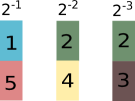
Example 2.

Consider a categorical distribution with rate parameters $\gamma_{1},\ldots,\gamma_{5}$ corresponding to five different events 0.5, 0.375, 0.125, 0.25 and 0.5. The sum of the rate parameters $\sum_{k=1}^{n}\gamma_{k}=1.75$. Figure 1 illustrates the line segments for the events. Say the point $x$ sampled on the line is 0.6, then, the event chosen will be the second (green in Figure 1) one corresponding to the rate parameter 0.375.

A key challenge that we face in using this standard approach is that, in our setting the sampling is without replacement. That is, as events occur, the rate parameter corresponding to that event is removed, and cannot be sampled again. Therefore, an update equivalent to removing a line segment would leave a “gap” or “hole”. A simple hack of filling the hole with the last end point would not work, as the line segments have varying lengths. It would require shifting all subsequent line segments to cover the gap, which is computationally expensive. This naïve approach turns out to be extremely inefficient in our setting. To ensure an efficient implementation of our model, our goal is to be able to sample in $\operatorname{O}(1)$ time.

Therefore, we need to design a new, efficient method for sampling a categorical distribution which undergoes frequent updates, owing to sampling without replacement. In our setting, these updates reflect the addition and removal of potential activation and deactivation events. We make two simple but important observations that motivate the design of our sampling method.
1) If we divide each line segment into smaller “shards”, the sampling process would be statistically equivalent to that from the original categorical distribution, as long as the sum of the lengths of these shards is equal to the original segment.
2) If the length of the line segment for each event is the same, we can simply replace an event that we want to remove with the last one.

Data Structure. We choose to represent the categorical distribution as a set of $m$ arrays. Each array corresponds to a fixed shard length from $2^{-1},\ldots,2^{-m}$. For instance, say $m=3$, the 3 arrays would correspond to shards of length $0.5,0.25,0.125$ respectively. Intuitively, $m$ can be viewed as the precision of the rate parameter when using the array representation. In particular, $m$ decides the granularity of shards, since the smallest shard that a line segment is divided into is of length $2^{-m}$. A line segment corresponding to a rate parameter may be divided into shards of different lengths, and hence may be present in multiple arrays. Furthermore, since the elements of each array are of equal length (length $2^{-i}$ for the $t^{th}$ array), the total length of the array can be easily determined by simply maintaining the count of elements in the array. Let $c_{i}$ denote the count or number of elements in array $i$. Then, the length of array $i$ is $2^{-i}\times c_{i}$.

Example 3.

Figure 2 shows the array representation of the categorical distribution from Example 2, for $m=3$ arrays (to ensure fine granularity we use $m=20$ in our implementation). Event 1 with $\gamma_{1}=0.5$ belongs completely to array corresponding to $2^{-1}$, while Event 2 with $\gamma_{1}=0.375$ is broken into shards of length $0.25,0.125$ and hence is present in arrays corresponding to $2^{-2},2^{-3}$. Further, we can consider array 1 as covering the interval (0,1] as it contains two shards ($c_{1}=2$) of length $2^{-1}$. Similarly, arrays 2 and 3 cover the intervals (1,1.5] and (1.5,1.75], respectively. Purely for clarity, we can think of sharding as mapping the $m$ arrays to a table of $m$ columns and $n$ rows as illustrated by Table 1 for the categorical distribution in Example 2. The arrays are a sparse representation of the table.

Event Id	$\gamma$	Columns
		$2^{-1}$	$2^{-2}$	$2^{-3}$
1	0.5	1	0	0
2	0.375	0	1	1
3	0.125	0	0	1
4	0.25	0	1	0
5	0.5	1	0	0
Total	$\sum_{k}\gamma_{k}=1.75$	$c_{1}$=2	$c_{2}$=2	$c_{3}$= 2

Table 1: Tabular representation of arrays of shards in Figure 2

Sampling. As before the first step in sampling is to pick a number $x$ uniformly at random from the interval $(0,\sum_{k}\gamma_{k}]$. Notice that this interval is equal to $(0,\sum_{i}2^{-i}\times c_{i}]$ in the array representation. We have a two step process to determine which event the sampled point $x$ maps to. First, find the $i^{th}$ array in which $x$ lies. Second, find the $j^{th}$ event in that array to be chosen as the sampled event.

As described above, the length of the $i^{th}$ array is $2^{-i}\times c_{i}$. Assuming $c_{0}=0$, the $i^{th}$ array to which $x$ belongs is the one that satisfies:

$$2^{-(i-1)}\times c_{i-1}<x\leq 2^{-i}\times c_{i}$$ (1)

Next, we find the index $j$ of the event chosen from array $i$ as:

$$j=\Bigg{\lceil}\frac{x-2^{-(i-1)}\times c_{i-1}}{2^{-i}\times c_{i}-2^{-(i-1)}\times c_{i-1}}\times c_{i}\Bigg{\rceil}$$ (2)

Example 4.

Say $x=1.3$, then it lies in the interval (1,1.5] covered by array 2, resulting in $i=2$. Then, $j=\big{\lceil}\frac{1.3-1}{1.5-1}\times 2\big{\rceil}=2$. The sampled event is then the second event in the second array in Figure 2, i.e., event 4.

Updates. Now, we show how our array representation helps prevent the “holes” created by updates with the naïve approach. First, it is easy to see that an update involving an addition of an event is trivial. Simply divide the line segment corresponding to the rate parameter of the event into shards, and append the shards to the end of the corresponding arrays. Now, if the update involves an event being removed because it has occurred, we need to find elements in all arrays that correspond to that event, and replace those elements with the last element in the corresponding arrays. In order to efficiently find all the indices at which an event lies in different arrays, a mapping of positions of an event in different arrays can be maintained in memory. Finally, $c_{i}$ of each array $i$ that was updated is changed to reflect the new counts. Notice that all shards in an array are of equal length, so shards can be replaced without resulting in gaps in the arrays.

Example 5.

Say the event 2 was sampled from the distribution by determining that $i=2$ and $j=1$. We keep track of each event’s associated positions in all arrays, so we know that event 2 lies in arrays $2,3$, and corresponds to index 1 for both arrays, as shown in this example. We replace the first element of arrays 2 and 3 with events 4 and 3 respectively, and update $c_{2}=1,c_{3}=1$.

Algorithm 1 ShardSampling

1:  $x\leftarrow$ a number sampled uniformly at random from $(0,\sum_{k=1}^{n}\gamma_{k}]$

2:  $i\leftarrow$ the array containing $x$ using Equation (1)

3:  $j\leftarrow$ the index in array $i$ determined using Equation (2)

4:  $e\leftarrow$ the chosen event at $j^{th}$ index in $i^{th}$ array

5:  Update arrays by replacing occurrences of $e$ with last element in respective arrays; update $c_{i}$s accordingly.

6:  Update the array positions for the set of events associated with the moved elements

7:  return  $e$

Algorithm 1 summarizes the proposed sampling procedure, that includes the sampling and update steps.

Running Time. Sampling $x$, and computing $j$ using Equation (2) takes constant time. We need $\operatorname{O}(\log m)$ time to compute $i$. Updating the arrays takes $\operatorname{O}(m)$ time. We store each event’s associated positions in all arrays, so step 4 takes $\operatorname{O}(1)$. The time to update events’ associated positions each time an event is updated is $\operatorname{O}(m)$. Therefore, sampling one event using our ShardSampling algorithm takes $\operatorname{O}(m)$ time. Obviously, the number of sampling actions performed in a propagation depend on several factors, such as, the size of the graph, the time horizon, and the seed set size. We discuss these factors in detail in our evaluation section.

6 Influence Maximization

Next, we discuss influence maximization, i.e., the process of seed selection to maximize the spread of influence under the CNP model. The influence maximization problem for non-progressive models is similar to that described in [22]. However, since nodes can deactivate, the spread, traditionally defined as the expected number of active nodes, changes with time. Thus, maximizing the expected number of active nodes at a given timestamp, or at the time horizon may not be ideal from the point of view of a company initiating a viral marketing campaign. We start by proposing an intuitive objective function for spread under a non-progressive model. Importantly, we show that our proposed spread function is monotone and submodular, hence the greedy approach yields a $(1-1/e)$-approximation to the optimal solution.

6.1 Objective Function

In a non-progressive world, an intuitive objective from the point of view of a marketer is to maximize the “active time” of its customers in a given social network. That is, maximize the total amount of time that nodes in the network are active, in expectation. Given a seed set $A$,

$$spread_{A}=\sum_{v\in V}\tau_{v}$$

where $\tau_{v}$ is the sum of time intervals within T for which node $v$ is active. Then, the influence maximization problem [22] is defined as: select a seed set of nodes $A\subseteq V$ to be activated such that the expected $spread_{A}$ is maximized over a chosen time horizon $T$, given the non-progressive influence propagation model.

6.2 Monotonicity and Submodularity

As an important step towards solving the influence maximization problem, we show that the expected $spread$ is monotone and submodular. Then, we can use the state-of-the-art greedy algorithm, such as CELF [24] and CELF++ [19], to guarantee a $(1-1/e)$-approximation. It is easy to see that,

$$\operatorname{E}[spread_{A}]=\sum_{v\in V}\operatorname{E}[\tau_{v}]=\int_{t=0}^{T}\operatorname{E}[\sigma(A,t)]dt$$

where $\sigma(A,t)=|S|$, $S$ is the set of nodes activated from the seed set $A$ at timestamp $t$, and $\sigma(A,t)$ is the number such nodes or the cardinality of set $S$. Therefore, we can prove monotonicity and submodularity of the expected spread, by showing that these properties hold for $\operatorname{E}[\sigma(A,t)]$. For this, we follow the proof guidelines in [22] to construct a deterministic possible world from the random process that we are modeling. Let $X$ be the set of all possible worlds, and given $x\in X$, let $pdf(x)$ denote the probability density function of $x$. Then,

$$\operatorname{E}[\sigma(A,t)]=\int_{x\in X}pdf(x)\times\sigma_{x}(A,t)dx$$

Thus, we only need to prove that $\sigma_{x}(A,t)$ is monotone and submodular. Note, that we need to integrate over the possible worlds, as opposed to a summation performed in [22], because the number of deterministic possible worlds is uncountable in our setting.

Lemma 1.

Additivity of spreads: Given two sets of seed nodes $A,B$, timestamp $t$, and a possible world $x$,

$$S_{x}(A\cup B,t)=S_{x}(A,t)\cup S_{x}(B,t)$$

where $S_{x}(A,t)$ denotes the set of nodes activated by seed set $A$ in possible world $x$ at timestamp $t$.

Theorem 1.

Given lemma 1, $\sigma_{x}(A,t)=|S_{x}(A,t)|$ is monotone and submodular.

Proof.

Assuming the additivity of spreads holds for sets $A$ and $B$, then by definition, $S_{x}(A\cup B,t)=S_{x}(A,t)\cup S_{x}(B,t)$. On adding a set $B$ to an initial set $A$, $|S_{x}(A\cup B,t)|=|S_{x}(A,t)\cup S_{x}(B,t)|\geq|S_{x}(A,t)|$ Hence, $|S_{x}(A,t)|$, equivalently $\sigma_{x}(A,t)$ is monotone.

For all sets $A\subseteq B$ and all nodes $v$, we need to show that,

$$|S_{x}(A\cup\{v\},t)-S_{x}(A,t)|\geq|S_{x}(B\cup\{v\},t)-S_{x}(B,t)|$$

By the additivity of spreads, $S_{x}(A\cup\{v\},t)=S_{x}(A,t)\cup S_{x}(\{v\},t)$. Then,

$$S_{x}(A\cup\{v\},t)-S_{x}(A,t) =S_{x}(A,t)\cup S_{x}(\{v\},t)-S_{x}(A,t)$$

$$=S_{x}(\{v\},t)-S_{x}(\{v\},t)\cap S_{x}(A,t)$$

Similarly, $S_{x}(B\cup\{v\},t)-S_{x}(B,t)=S_{x}(\{v\},t)-S_{x}(\{v\},t)\cap S_{x}(B,t)$. Since $A\subseteq B$, $S_{x}(A,t)\subseteq S_{x}(B,t)$, applying an intersection with $S_{x}(\{v\},t)$ on both sides, then subtracting from $S_{x}(\{v\},t)$, we get

$$S_{x}(\{v\},t)-S_{x}(\{v\},t)\cap S_{x}(A,t) \supseteq S_{x}(\{v\},t)-S_{x}(\{v\},t)\cap S_{x}(B,t)$$

$$S_{x}(A\cup\{v\},t)-S_{x}(A,t) \supseteq S_{x}(B\cup\{v\},t)-S_{x}(B,t)$$

$$|S_{x}(A\cup\{v\},t)-S_{x}(A,t)| \geq|S_{x}(B\cup\{v\},t)-S_{x}(B,t)|$$

Hence submodularity. ∎

(a) Deactivation rate - Flixster

(b) Activation rate - Flixster

(c) Deactivation rate - Flickr

(d) Activation rate - Flickr

Figure 3: Model Parameters for Flixster and Flickr Datasets

7 Experimental Evaluation

In this section we first describe how the edge weights of our model can be learned from data, and the details of our experimental setup. Next, we present the results of evaluating our model on real and synthetic datasets. We compare the accuracy and running time of: traditional IC model, state-of-the-art continuous time progressive model ConTinEst[11], DNP and CNP, for estimating the spread as defined in Section 6.1.

7.1 Learning model parameters

We divide each dataset into training and test sets. We use the training set to learn the different model parameters, i.e., deactivation rates and edge weights. The first challenge we face is identifying deactivations in common datasets. If we had access to logs associated with each activations and deactivations, for instance, timestamps for service subscriptions and unsubscribe actions, this would be trivial. However, such service subscription datasets are not publicly available.

7.1.1 Activation and Deactivation

Given a training set in the form of an action log with <user,action,timestamp> tuples, we would like to find the timestamps for activations and deactivations. We use the following proxy for defining events: 1) when a user performs an action we call it an activation event and mark the user active 2) at each activation we start a timer, the event of the timer running out before another activation occurs, is called a deactivation, and the user is said to be deactivated. The timer is set for a length equal to the deactivation time window. Similar definitions of active users are used by social networking services as a metric of the popularity of these sites. For instance, Facebook maintains statistics of its daily (and monthly) active users, where a day (resp., month) is the deactivation time window.

Deactivation time window. To find the value of the deactivation time window from the action log, we first get all the time gaps between two consecutive actions of each user in the training dataset. We ignore time gaps of less than one day to avoid the bias of a user performing multiple actions in a single session. We set the deactivation time window as the expected value (mean) of time gaps for all experiments. In addition, to be rigorous with our analysis, we also evaluate our model over different deactivation time windows in the next section.

Rate parameters. Using the above definition of activation and deactivation events, we now define the total active time for a node $u$ as the sum of time intervals for which node $u$ is active in our training set. Then, the deactivation rate parameter $\gamma_{-,u}$ for node $u$ is

$$deactivation\;rate(u)=\frac{number\;of\;deactivations(u)}{total\;active\;time\;(u)}$$

Finally, we define the rate parameters corresponding to edges which are responsible for activations. At each activation, we find the set of active neighbors of that node at that timestamp. Say, the node has $k$ active neighbors when it activates. We assign a contribution score of $1/k$ to each of the $k$ edges from an active neighbor. Then, the activation rate parameter $\gamma_{+,u,v}$ for edge $(u,v)$ is

$$activation\;rate(u,v)=\frac{\sum contribution\;score(u,v)}{total\;active\;time\;(u)}$$

We use these methods to learn the parameters of the CNP model. As described in Section 4.3, we can cast the rate parameters of CNP to probabilities for the DNP model, with the $\mathrm{CDF}$ of the exponential distribution.

IC model edge weights. The existing methods for IC model models are not scalable. Our approach is similar to the PCB method in [17]. This is essentially a counting argument and a recent paper [26] uses PCB to learn the edge weights for the IC model and report good accuracy w.r.t to the true edge weights, even better than the likelihood method of Saito et al. [32].

$$Probability(u,v)=\frac{\sum contribution\;score(u,v)}{number\;of\;activations\;(u)}$$

7.1.2 Global Influence

In real social networks, users may get influenced by external sources, such as the popular trends, news etc. We model such influences by inserting a “global node” and that has a directed edge to all users. This global node is always active, and influences all nodes equally. Technically, the influence from this global node is used to explain activation of a node $u$ that has no other active neighbors. Thus, we can compute its total contribution score over all its outgoing edges, and define the global influence value as:

$$\frac{total\;contribution\;score}{time\;horizon\times number\;of\;nodes\;in\;the\;graph}$$

7.2 Datasets

We evaluate our model on synthetically generated data and two real datasets: Flixster and Flickr, for which we have a social network, and an action log which contains the timestamps of users’ actions.

Synthetic. We generate a random 500 node unweighted forest fire network. We artificially generate cascades and deactivation events. For generating cascades, we pick a node at random and randomly generate a timestamp at which this node performs an action and hence becomes active. To avoid the dependence of cascade generation on any underlying diffusion model, we randomly choose a neighbor and sample a random activation time for it. We repeat this process recursively to generate the cascades. For the deactivation events too, we randomly select a node and make it inactive at a random timestamp.

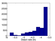
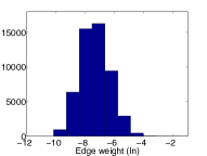
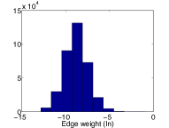
Flixster. Flixster is a movie rating service, where users form an explicit social network. Our dataset [21] has 1 million nodes (users) and 26.7 million edges (social connections). An activation event is the act of rating a movie from a specific genre (horror in our experiments). We divide the action log into one year training and one year test set. Using the expectation of intervals between consecutive actions as the deactivation time window, we find it to be 38 days for our dataset. The distribution of rate parameters are shown in Figures 3(a) and 3(b), as computed using the approach described above, and the global influence value for this dataset is $2.095\times 10^{-5}$.

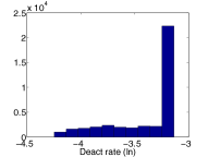
Flickr. Our second dataset comes from the photo sharing service of Flickr. The dataset [6] has 2.3 million nodes and 33.1 million edges. An action corresponds to using the “favorite photo” feature, i.e., marking a photo as favorite. The associated action log is over 138 days, of which we use the first 70 days as our training set for learning parameters, and the next 68 days as our test set. The deactivation time window is 23 days and the global influence value for our dataset is $1.415\times 10^{-4}$. Figures 3(c) and 3(d) show the distribution of rate parameters for Flickr.

(a) Error in Spread estimation

(b) Running time

Figure 4: Spread estimation error and time comparison for progressive (IC, ConTinEst) and non-progressive models (DNP, CNP) for Flixster dataset

Dataset	Ground	CNP	DNP	ConTinEst	IC
	Truth			[11]
Flixster	964013	949750	991141	2477678	2833860
		(1.5%)	(2.8%)	(157%)	(194%)
Flickr	2435663	2432053	2409695	4423372	4922860
		(0.148%)	(1.07%)	(81%)	(102%)

Table 2: Spread estimated by progressive (IC, ConTinEst) and non-progressive models (DNP, CNP) and error percentage w.r.t. ground truth

7.3 Comparison Across Models

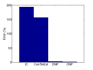
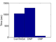
We start with presenting an overview of our results comparing different models: progressive vs. non-progressive models, and discrete vs. continuous time models, across two axes: accuracy of spread estimation and running time. Figure 4 illustrates this comparison for Flixster dataset. See detailed numbers for both datasets in Table 2. We make the following key observations, and substantiate these with details through the remainder of this section.

• Progressive models, here classical IC model and state-of-the-art ConTinEst, overestimate the spread and result in an error of 80-194% compared with the ground truth.

• Non-progressive models, DNP and CNP, are highly accurate in estimating the spread with very small errors of 0.1-3%. Notice that DNP is the non-progressive counterpart of the progressive IC model model and improves the accuracy or error in estimating spread by a 100%.

• Continuous models ConTinEst and CNP are slightly better at estimating accuracy than the discrete models IC and DNP.

• Our model CNP is not just more accurate but also an order of magnitude faster than the state-of-the-art continuous time model ConTinEst (Figure 4(b)). These results are for running 100 Monte-Carlo simulations.

(a) Error in Spread estimation for synthetic data

(b) Running time of ConTinEst vs. CNP on real data

Figure 5: Accuracy comparison for progressive (IC, ConTinEst) and non-progressive models (DNP, CNP)

Evaluating Accuracy. We evaluate the accuracy of the estimation of spread of our model by simulating the propagation, starting at the state of the network at the last timestamp in our training set, and evaluating against the ground truth of spread achieved in the test set. In other words, the nodes active at the end of the training set are treated as the seed set, and the propagation is run for the time horizon equal to the length of the test set. The ground truth of spread is computed as the total active time of all nodes for the test set. Table 2 shows the spread as estimated by our model compared with the ground truth. For our model, error in spread estimation is just 1.5% and 0.1% over the Flixster and Flickr datasets resp. The difference between IC model and non-progressive models is two orders of magnitude. This validates that deactivation occurs in real datasets, and that modeling deactivation properly is critical for a reasonable estimation of influence spread in non-progressive settings.

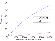
Next, we perform an experiment on synthetic data to show the impact of number of deactivations on the spread estimates by a progressive model (ConTinEst [11]) and our CNP model. Figure 6(a) shows this the error (%) in estimating the spread. As the deactivations increase, the gap in the accuracy of the two methods increase, with CNP performing over 83% better than the competitor, establishing that in the presence of deactivations, non-progressive phenomena are modeled accurately by CNP.

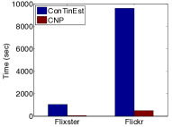
Evaluating Computational Cost. We compare the running time of ConTinEst with CNP for our two real datasets Flickr and Flixster for running 100 Monte-Carlo simulations. As seen in Figure 7(a), our model is an order of magnitude faster than its progressive competitor.

(a) Varying $\#$ deactivations Synthetic data

(b) Varying deactivation rate Flixster

(c) Varying deactivation rate Flickr

(d) Varying deactivation time window Flixster

Figure 6: Accuracy comparison for progressive (IC, ConTinEst) and non-progressive models (DNP, CNP) with varying deactivation parameters

7.4 Varying Parameter Values

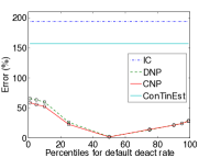
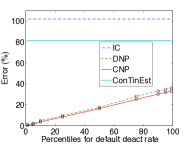
Effect of deactivation parameters on accuracy. For Flickr, we observe that 98% of the nodes perform no action in our training set, and hence get a zero deactivation rate. This is an artifact of the short timespan of the training data. Filtering those nodes would result in a disconnected graph. To overcome this shortcoming of the data sample and to avoid overfitting, we assign a default deactivation rate to all such nodes. We use the set of non-zero deactivation rates (as learned from the data) as a guideline, and test different percentiles of this set as the default deactivation rate. Instead of fixing the value, we evaluate its impact on the accuracy by varying it, as shown in Figure 6(b) for Flixster dataset. As seen in the figure, the default deactivation rate does impact the accuracy slightly, still the estimates by CNP are orders of magnitude more accurate than IC model and ConTinEst. Also notice that the estimated spread for DNP and CNP is very similar validating our argument in Section 4.3 that DNP is an approximation of CNP. The plots for Flickr are skipped for brevity, but the methodology adopted and results were similar. For the remainder of the experiments we set the default deactivation rate for Flixster and Flickr to the best obtained, i.e., $50^{th}$ and 1 percentile resp. of the unique non-zero deactivation rates learned.

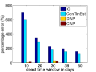
Next, we show using Figure 6(d) that changing the deactivation time window does not significantly impact the accuracy of CNP model. Although the progressive models are unaffected by the deactivation window, the ground truth computed is different across windows, and this change is reflected in the error percentage.

Effect of varying parameters on running time.

(a) Running time of ConTinEst vs. CNP

(b) Increasing time horizon Flickr

(c) Increasing time horizon Flixster

(d) Increasing graph size Flixster

Figure 7: Running time comparisons for non-progressive models: DNP and CNP

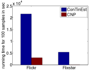
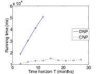
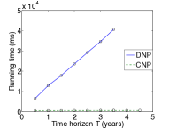
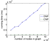
First, we compare the running time of ConTinEst with CNP, as seen in Figure 7(a), our model is an order of magnitude faster than its progressive competitor. Next, comparing the non-progressive models. The two factors that affect the computational cost of simulating the non-progressive models are: time horizon and graph size. We compare the computational cost for CNP and DNP for increasing time horizon on the full graphs of the two datasets. As seen in Figure 7(c), the running time for DNP increases linearly over increasing time horizon, while that for CNP changes only slightly. For instance, for Flickr, the running time for CNP is 73% less than DNP at 27 month time horizon. Finally, we set time horizon as 2 years for Flixster and show the running time with increasing graph size in Figure 7(d). Again, CNP scales up very well. The results for Flickr were similar and skipped for brevity.

Progressive Setting. We ask the question, “What if the world is progressive, i.e., there are no deactivations, how well would CNP perform?” To this end we perform an experiment of setting the deactivation time window to the end of the time horizon, essentially saying no nodes deactivate. We then compare this model we call CP for the continuous progressive version of our proposed model against ConTinEst and CNP. We observe that the running time on Flixster for CP, CNP and ConTinEst are 60, 64 and 1041s resp. The running time results for Flickr for the CP, CNP and ConTinEst were 498, 606 and 9605s resp. This illustrates that despite the data being progressive in nature, our model is 17-20 times faster than the state-of-the-art progressive continuous model.

8 Conclusions

There are applications where the propagation phenomena are more accurately captured using non-progressive models. In their seminal paper, Kempe et al. [22] proposed a non-progressive LT model and showed that over any finite time horizon of interest, its behavior can be effectively simulated by a progressive model with the given social graph replicated at every timestamp in the horizon. Inspired by this, we proposed a non-progressive model and showed that its behavior over a time horizon can be simulated without any need for graph replication. The resulting discrete time non-progressive model is still not scalable owing to the prohibitive number of samplings necessary in order to monitor the state of nodes at every time. We proposed an alternative continuous time non-progressive model and showed that it permits a highly efficient implementation. We developed an efficient sampling strategy to further improve the efficiency of our continuous time model.In place of expected number of active nodes, for our continuous time model, we motivated the expected total amount of time the nodes in the network are active, as the right notion of spread, which a seed selection algorithm should optimize. We showed that this objective function is monotone and submodular in the set of seed nodes. By extensive experiments on two data sets, we show that our model significantly outperforms the state of the art progressive model ConTinEst [11] both on accuracy of spread estimating and on running time. It would be interesting to study non-progressive continuous time models in the competitive setting, where competitors may be adversarial.

Proof of Lemma 1. We now show that in the construction of possible worlds, lemma 1 holds for any two spreads. Given a possible world $x$, a seed set $A$, the influence propagation is deterministic. That is, each activation and deactivation event has a timestamp associated with it, and the propagation can be viewed as a sequence of activations and deactivations. In this deterministic setting, we can use mathematical induction to prove this lemma.

First, we consider the base case at time zero, $S_{x}(A,0)=A$. Then, $S_{x}(A\cup B,0)=A\cup B=S_{x}(A,0)\cup S_{x}(B,0)$. Hence, the property holds for this base case.

Next, we find the next smallest number in all the schedules. Let $t$ be the timestamp when the next event happens. Say, $S_{x}(A\cup B,t-\delta)=S_{x}(A,t-\delta)\cup S_{x}(B,t-\delta)$ holds, where $\delta$ is a very small number. Then, at timestamp $t$, an event happens. The event can either be an activation or a deactivation. We consider each of the 10 possible scenarios, the first 7 correspond to activations and the next 3 to deactivations. For any edge $v\rightarrow u$ , in the possible world $x$, we sampled an activation at timestamp $t$, then,

Case 1. when $u$ is in both $S_{x}(A,t-\delta)$ and $S_{x}(B,t-\delta)$, there is no activation in the possible world x.

Case 2. when $v$ is in both $S_{x}(A,t-\delta)$ and $S_{x}(B,t-\delta)$, i.e., $v$ is in $S_{x}(A\cup B,t-\delta)$, but $u$ is in neither of them, then after timestamp $t$, $u$ is in $S_{x}(A,t),S_{x}(B,t)$ and $S_{x}(A\cup B,t)$. Thus, $S_{x}(A\cup B,t)=S_{x}(A,t)\cup S_{x}(B,t)$ after the event.

Case 3. $v$ is in both $S_{x}(A,t-\delta)$ and $S_{x}(B,t-\delta)$, however, $u$ is in only one of them, without loss of generality, say $u$ is in $S_{x}(A,t-\delta)$. Since $S_{x}(A\cup B,t-\delta)=S_{x}(A,t-\delta)\cup S_{x}(B,t-\delta)$, $v$ and $u$ are in $S_{x}(A\cup B,t-\delta)$. After the event, $u$ is in $S_{x}(A,t),S_{x}(B,t)$ and $S_{x}(A\cup B,t)$, therfore, $S_{x}(A\cup B,t)=S_{x}(A,t)\cup S_{x}(B,t)$. Case 4. when $v$ is in one of $S_{x}(A,t-\delta)$ and $S_{x}(B,t-\delta)$, without loss of generality, say $v$ is in $S_{x}(A,t-\delta)$ , however, $u$ is in neither of them. Now, $v$ is in $S_{x}(A\cup B,t-\delta)$ and after the event, $u$ is in $S_{x}(A,t)$ and $S_{x}(A\cup B,t)$. Then after the event, $S_{x}(A\cup B,t)=S_{x}(A,t)\cup S_{x}(B,t)$.

Case 5. when both $v$ and $u$ are in $S_{x}(A,t-\delta)$ but not in $S_{x}(B,t-\delta)$. Then, both $v$ and $u$ are also in $S_{x}(A\cup B,t-\delta)$. The event does not result in any changes.

Case 6. when $v$ is in $S_{x}(A,t-\delta)$ but not in $S_{x}(B,t-\delta)$, and $u$ is in $S_{x}(B,t-\delta)$ but not in $S_{x}(A,t-\delta)$, i.e., $u$ is in $S_{x}(A\cup B,t-\delta)$. After the event, $u$ is in $S_{x}(A,t)$, $S_{x}(B,t)$ and $S_{x}(A\cup B,t)$, thus, $S_{x}(A\cup B,t)=S_{x}(A,t)\cup S_{x}(B,t)$. Case 7. when $v$ is in neither of $S_{x}(A,t-\delta)$ and $S_{x}(B,t-\delta)$. No change happens after the event, and $S_{x}(A\cup B,t)=S_{x}(A,t)\cup S_{x}(B,t)$ holds.

Case 8. when $v$ is in both $S_{x}(A,t-\delta)$ and $S_{x}(B,t-\delta)$. After the event, $v$ is not in $S_{x}(A,t)$, $S_{x}(B,t)$ and $S_{x}(B\cup A,t)$, thus, $S_{x}(A\cup B,t)=S_{x}(A,t)\cup S_{x}(B,t)$. Case 9. when $v$ is in one of $S_{x}(A,t-\delta)$ or $S_{x}(B,t-\delta)$. After the event, $v$ is not in $S_{x}(A,t)$, $S_{x}(B,t)$ and $S_{x}(B\cup A,t)$, hence, $S_{x}(A\cup B,t)=S_{x}(A,t)\cup S_{x}(B,t).$ Case 10. when $v$ is neither in $S_{x}(A,t-\delta)$ nor $S_{x}(B,t-\delta)$. No change happens after the event.

In each of the above cases, $S_{x}(A\cup B,t)=S_{x}(A,t)\cup S_{x}(B,t)$ after the event. By mathematical induction, $S_{x}(A\cup B,t)=S_{x}(A,t)\cup S_{x}(B,t)$. Therefore, the objective function in our model is monotone and submodular. ∎

References

- [1] J. G. U. A. Ostfeld and E. Salomons. Battle of water sensor networks: A design challenge for engineers and algorithms. In WSDA, 2006.
- [2] S. Bharathi, D. Kempe, and M. Salek. Competitive influence maximization in social networks. In WINE, 2007.
- [3] G.-I. Bischi and U. Merlone. Global dynamics in adaptive models of collective choice with social influence. In Mathematical modeling of collective behavior in socio-economic and life sciences, pages 223–244. Springer, 2010.
- [4] L. Blume. The statistical mechanics of strategic interaction. Games and Economic behavior, 1993.
- [5] C. Budak, D. Agrawal, and A. E. Abbadi. Limiting the spread of misinformation in social networks. In WWW’11.
- [6] M. Cha, A. Mislove, and P. K. Gummadi. A measurement-driven analysis of information propagation in the flickr social network. In WWW, 2009.
- [7] W. Chen, L. V. S. Lakshmanan, and C. Castillo. Information and Influence Propagation in Social Networks. Synthesis Lectures on Data Management. Morgan & Claypool Publishers, 2013.
- [8] W. Chen, Y. Wang, and S. Yang. Effcient influence maximization in social networks. In KDD, 2009.
- [9] W. Chen, Y. Wang, and L. Zhang. Scalable influence maximization in social networks under linear threshold model. In ICDM, 2010.
- [10] P. Domingos and M. Richardson. Mining the network value of customers. In KDD, 2001.
- [11] N. Du, L. Song, M. Gomez-rodriguez, and H. Zha. Scalable influence estimation in continuous-time diffusion networks. In NIPS. 2013.
- [12] G. Ellison. Learning, local interaction, and coordination. Econometrica, 1993.
- [13] E. Even-Dar and A. Shapira. A note on maximizing the spread of influence in social networks. In Internet and Network Economics, volume 4858. Springer Berlin Heidelberg, 2007.
- [14] M. Fazli, M. Godsi, J. Habibi, P. J. Khalilabadi, V. Mirrokni, and S. S. Sadeghabad. On the non-progressive spread of influence through social networks. In LATIN’12.
- [15] A. Ganesh, L. Massoulié, and D. Towsley. The effect of network topology on the spread of epidemics. In INFOCOM 2005. 24th Annual Joint Conference of the IEEE Computer and Communications Societies. Proceedings IEEE, volume 2, pages 1455–1466. IEEE, 2005.
- [16] M. Gomez-Rodriguez and B. Scholkopf. Influence maximization in continuous time diffusion networks. In ICML, 2012.
- [17] A. Goyal, F. Bonchi, and L. V. Lakshmanan. Learning influence probabilities in social networks. In WSDM, 2010.
- [18] A. Goyal, F. Bonchi, and L. V. S. Lakshmanan. A data-based approach to social influence maximization. Proc. VLDB Endow., 2011.
- [19] A. Goyal, W. Lu, and L. V. Lakshmanan. Celf++:optimizing the greedy algorithm for influence maximization in social networks. In WWW, 2011.
- [20] M. Jackson and L. Yariv. Diffusion on soical networks. In Public Economy Theory Meeting, Marseille, 2005.
- [21] M. Jamali and M. Ester. A matrix factorization technique with trust propagation for recommendation in social networks. In RecSys, 2010.
- [22] D. Kempe, J. Kleinbery, and E. Tardos. Maximizing the spread of influence through a social network. In KDD, 2003.
- [23] C. Kuhlman, V. Kumar, M. Marathe, S. Swarup, G. Tuli, S. Ravi, and D. Rosenkrantz. Inhibiting the diffusion of contagions in bi-threshold systems: Analytical and experimental results. In Proceedings of the AAAI Fall 2011 Symposium on Complex Adaptive Systems (CAS-AAAI 2011), pages 91–100, 2011.
- [24] J. Leskovec, A. Kraus, C. Guestrin, C. Faloutsos, J. M. VanBriesen, and N. S. Glance. Cost-efficiective outbreak detection in networks. In KDD, 2007.
- [25] Y. Li, W. Chen, Y. Wang, and Z.-L. Zhang. Influence diffusion dynamics and influence maximization in social networks with friend and foe relationships. In WSDM, 2013.
- [26] S. Lin, F. Wang, Q. Hu, and P. S. Yu. Extracting social events for learning better information diffusion models. In KDD, 2013.
- [27] Y. Matias, J. S. Vitter, and W.-C. Ni. Dynamic generation of discrete random variates. In SODA, pages 361–370, 1993.
- [28] M. F. B. Nan Du, Yingyu Liang and L. Song. Continuous-time influence maximization for multiple items. CoRR, abs/1312.2164, 2013.
- [29] A. Ostfeld and E. Salomons. Optimal layout of early warning detection stations for water distribution systems security. In J. Water Resources Planning and Management, 2004.
- [30] N. Pathak, A. Banerjee, and J. Srivastava. A generalized linear threshold model for multiple cascades. In ICDM, 2010.
- [31] B. A. Prakash, D. Chakrabarti, N. C. Valler, M. Faloutsos, and C. Faloutsos. Threshold conditions for arbitrary cascade models on arbitrary networks. Knowledge and information systems, 33(3):549–575, 2012.
- [32] K. Saito, R. Nakano, and M. Kimura. Prediction of information diffusion probabilities for independent cascade model. In Knowledge-Based Intelligent Information and Engineering Systems. Springer, 2008.
- [33] A. D. Sarma, S. Gollapudi, R. Panigrahy, and L. Zhang. Understanding cyclic trends in social choices. In WSDM, pages 593–602, 2012.
- [34] R. Schenkel, T. Crecelius, M. Kacimi, S. Michel, T. Neumann, J. X. Parreira, and G. Weikum. Efficient top-k querying over social-tagging networks. In SIGIR’08.
- [35] T. Valente. Network models and methods for studying the diffusion of innovations. In Models and methods in social network analysis. Cambridge Univ. Press, 2005.