Analytical Expression of Genuine Tripartite Quantum Discord for Symmetrical X-states

Abstract

The study of classical and quantum correlations in bipartite and multipartite systems is crucial for the development of quantum information theory. Among the quantifiers adopted in tripartite systems, the genuine tripartite quantum discord (GTQD), estimating the amount of quantum correlations shared among all the subsystems, plays a key role since it represents the natural extension of quantum discord used in bipartite systems. In this paper, we derive an analytical expression of GTQD for three-qubit systems characterized by a subclass of symmetrical X-states. Our approach has been tested on both GHZ and maximally mixed states reproducing the expected results. Furthermore, we believe that the procedure here developed constitutes a valid guideline to investigate quantum correlations in form of discord in more general multipartite systems.

1 INTRODUCTION

Quantum correlations are assuming increasing relevance, since they can be exploited to improve our ability to perform many informational and computational tasks SEPARAB_ENTGNL_1QUBIT ; SEPARAB_ENTGN_CORR ; SEPAR_QDISC_1QUBIT ; SEPAR_QUANT_COMP_WO_ENTNGL . Therefore, the problem of their characterization and quantification has become a significant topic of research. Traditionally, the most used form of quantum correlation is entanglement, and the development of quantum information theory is fundamentally due to its implementation in information and communication protocols NIELSEN_CHUANG ; HORODECKI_REVIEW_ENTANGLEMENT .

A form of quantum correlation other than entanglement is quantum discord (QD) ZUR_DISC ; H_VEDR ; LUO_QBIT , which can be expressed in terms of the difference between the total and the classical correlations for a system when one of its subparties is subject to an unobserved measure process. Such a quantity, however, significantly depends upon both the subsystem chosen and the measurement performed on it: in particular, if the measurement is carefully selected, we can minimize its “disturbing effect” on the system LUO_MEAS . This choice corresponds to the minimization of QD firstly over a set of possible measurements (on a fixed subsystem), typically projective von Neumann measurements LUO_MEAS ; ZUR_DISC , and secondly over all possible subsystem on which the local measurement can be performed. Recent efforts in the study of the optimization processes have led to analytical expression for quantum discord in some particular LUO_QBIT and more general states GIROLAMI_ANAL_PROGR_DISC_2Q ; QD_ARB_ST2 in systems composed of two qubits.

Both entanglement and QD have widely been analyzed and used in bipartite systems, while their extension to multipartite systems is still discussed and tackled with different approaches BENNET_MULTIP_POSTUL ; RULLI_MULTIP_GLOBAL_QDISC ; Xu_GLOBAL_QDISC_ANAL ; CHAKRA_QDISS_3QBIT ; GIORGI_GENUIN_MULTIP . For instance, Vinjanampathy et al. Vinja_Rau_QBIT-QDIT proposed a method to evaluate analytically quantum discord for a n-partite system of qubits in some special cases, but they treated the whole system as a bipartite one (each subparty containing $1$ or $n-1$ qubits, respectively). On the other hand, Giorgi et al. GIORGI_GENUIN_MULTIP defined, for a n-partite system, genuine n-partite correlations, which can be divided into total, classical or quantum. These kinds of correlations are shared between all the n parties which form the system, i.e. they cannot be accounted for considering any of the possible subsystems. The quantum part of genuine correlations is quantified by genuine n-partite quantum discord. The approach of Ref. GIORGI_GENUIN_MULTIP represents a natural extension of the concept of QD as introduced for bipartite systems, and this is the reason why we will follow it in the present work. However, it requires massive numerical optimization procedures over a number of parameters, thus making the calculations very demanding Yichen_QD_NPCOMPLETE . Therefore, the application of such a criterion is not easily amenable.

This justifies the scarce number of works investigating the time evolution of quantum correlations in multipartite system coupled to noisy environments. Specifically only few cases have been considered: two level systems undergoing random telegraph noise FABRIZIO_GENUIN ; THEO_GEN_MULTIP_CORR and quantum phase transitions in spin systems EXP_MULTIP_OPSYS ; EXP_MULTIP_SPINCHAIN ; EXP_MULTIP_XXZModel .

The purpose of this paper is to derive an analytical expression for the genuine tripartite quantum discord (GTQD) for a class of three qubits systems. In detail, we will focus on those systems described by X-states, which play a relevant role in a large number of physical systems and allow for easy calculations of certain entanglement measures WEINST_TRIP_ENTANGL ; WEINSTEIN_ENTNGL_3Q_X . X-states have been widely investigated also in bipartite systems, where an analytical expression for QD has been proposed in ANAL_QD_2QUBIT_X_states . However, this approach has been questioned, since it is not always providing the correct result Lu_counterxample_Ali_X_states_QD ; Chen_Zang_QD_2qubit_Xstates ; Yichen_QD_X_states_Symm_ERRORS .

The paper is organized as follows. In Sec. 2 we introduce the genuine quantifiers for correlations in multipartite quantum systems. In Sec. 3 we introduce the expression for a symmetrical tripartite X-state and derive some constraints on its defining parameters. In Sec. 4 we estimate all the quantities required to compute GTQD, and in particular we describe the optimization procedures (both numerical and analytical) appearing in the expression of GTQD. Sec. 5 concerns the comparison between our results on GTQD and others already present in the literature and, finally, in Sec. 6 we draw conclusions.

2 QUANTIFIERS FOR GENUINE TRIPARTITE CORRELATIONS

Here we illustrate the correlation measures adopted in this work to quantify tripartite quantum discord and entanglement.

2.1 Tripartite Quantum Discord

In a tripartite system, described by a state $\rho=\rho_{A,B,C}$, the tripartite quantum mutual information is obtained as a generalization of the quantum mutual information for bipartite systems Vedr_REL_ENTR ; Modi_UNIFIED_QUANT_CLASS_CORR ; GIORGI_GENUIN_MULTIP ; WALCZAK_MULTIPARTITE :

$$T(\rho)=S(\rho_{A})+S(\rho_{B})+S(\rho_{C})-S(\rho),$$ (1)

and represents the total amount of correlations encoded in this system. Here $S(\rho)=-\mathrm{Tr}[\rho\log_{2}(\rho)]$ is the von Neumann entropy, and $\rho_{i}$ $(i=A,B,C)$ is the reduced density matrix for the subsystem $i$. Following the same procedure used in the literature for bipartite systems ZUR_DISC , Giorgi et al. GIORGI_GENUIN_MULTIP define the tripartite classical correlations in the system as the quantum version (of a classical analogue) of the mutual information derived from the Bayes’ rule:

$$J(\rho)=\underset{i,j,k\in\{A,B,C\}}{\max}[S(\rho_{i})-S(\rho_{i|j})+S(\rho_{k})-S(\rho_{k|ij})],$$ (2)

which has been optimized over the indices $i,j,k$ in the set of all the possible permutation of subsystems $\{A,B,C\}$. Here $S(\rho_{i|j})$ and $S(\rho_{k|ij})$ are relative entropies and $\rho_{i|j}$ and $\rho_{k|ij}$ are the density matrices after a measurement on the subsystem $i$ or after a measurement on both subsystems $i$ and $j$, respectively FABRIZIO_GENUIN . We refer the reader to the Appendix A for a detailed definition of the relative entropies and their optimization. Like for bipartite systems, the tripartite quantum discord is given by the difference between total and classical correlations:

$$D(\rho)=T(\rho)-J(\rho).$$ (3)

However, among the correlations included in $T(\rho)$, a subset is shared by all of the three subsystems (genuine tripartite mutual information), and can be estimated as:

$$T^{(3)}(\rho)=T(\rho)-T^{(2)}(\rho),$$ (4)

where $T^{(2)}(\rho)$ is the maximum amount of mutual information shared by any couple of subsystems:

$$T^{(2)}(\rho)=\max[I(\rho_{A,B}),I(\rho_{A,C}),I(\rho_{B,C})],$$ (5)

where $I(\rho_{AB})=S(\rho_{A})+S(\rho_{B})-S(\rho_{AB})$. Since all the correlations that cannot be accounted for by $T^{(2)}(\rho)$ must be shared between all of the three subsystems, we can conclude that $T^{(3)}(\rho)$ measures the distance between $\rho$ and the closest product state along any bipartite cut of the system. Indeed it can be shown that $T^{(3)}(\rho)=\min[I(\rho_{AB,C}),I(\rho_{AC,B}),I(\rho_{BC,A})]$ (see Ref. GIORGI_GENUIN_MULTIP ).

Analogously, the genuine tripartite classical correlations reads:

$$J^{(3)}(\rho)=J(\rho)-J^{(2)}(\rho),$$ (6)

and GTQD:

$$D^{(3)}(\rho)=D(\rho)-D^{(2)}(\rho),$$ (7)

where:

$$J^{(2)}(\rho)=\max[J(\rho_{A,B}),J(\rho_{A,C}),J(\rho_{B,C})],$$ (8)

$$D^{(2)}(\rho)=\min[D(\rho_{A,B}),D(\rho_{A,C}),D(\rho_{B,C})].$$ (9)

Eqs. (4), (6) and (7) can be significantly simplified for the case of a state $\rho$ symmetrical under any exchange of its subsystems. Indeed it can be shown that FABRIZIO_GENUIN :

$$T^{(3)}(\rho)=I(\rho_{A,BC})=S(\rho_{A})+S(\rho_{A,B})-S(\rho),$$ (10)

$$D^{(3)}(\rho)=S(\rho_{A|BC})+S(\rho_{A,B})-S(\rho),$$ (11)

$$J^{(3)}(\rho)=S(\rho_{A})-S(\rho_{A|BC}).$$ (12)

2.2 Tripartite Negativity

In tripartite systems, represented by a state $\rho$, we can detect the presence of entanglement between subsystems by using the negativity $N$, which is defined as follows Vidal_Negativity :

$$N(\rho^{tC})=\sum_{i}|\lambda_{i}(\rho^{tC})|-1.$$ (13)

In the previous expression, $\rho^{tC}$ is the partial transpose of $\rho$ with respect to the subsystem $C$, and $\lambda_{i}(\rho^{tC})$ are the eigenvalues of $\rho^{tC}$. The negativity can be equivalently interpreted as the sum of the absolute values of the negative eigenvalues of $\rho^{tC}$ Vidal_Negativity , and it depends upon the subsystem on which we make the partial transpose of $\rho$.

When negativity is higher than zero, we can conclude that there is an entanglement between the subsystem $C$ and the compound subsystem $A-B$, but the converse is not necessarily true. Starting from this point, we can define the tripartite negativity as follows Sabin_Trip_Negat :

$$N^{(3)}(\rho)=\sqrt[3]{N(\rho^{tA})N(\rho^{tB})N(\rho^{tC})},$$ (14)

and this quantifier will be different from zero only when the entanglement is shared among all of the three subsystems, i.e. it is a “full” tripartite entanglement Sabin_Trip_Negat . However, apart from pure states, a null negativity could indeed not imply the absence of entanglement. Moreover, we must notice that tripartite negativity cannot distinguish the entanglement of a genuine tripartite entangled state from that of a biseparable state in a generalized sense Sabin_Trip_Negat ; EXP_MULTIP_SPINCHAIN . For tripartite systems that are symmetrical under any exchange of their qubits, as in our case of study, the tripartite negativity and the negativity always coincide:

$$N^{(3)}(\rho)=N(\rho^{tA})=N(\rho^{tB})=N(\rho^{tC}).$$ (15)

Another possible quantifier for tripartite entanglement is the three-tangle COFFMAN_Three_Tangle , but in this work we use negativity since the three-tangle is not able to detect tripartite entanglement for all states, e.g. W states Dur_Vidal_W_and_GHZ . However, it should be noticed that $N^{(3)}$ in this work is used simply to provide a further comparison with the outcomes of GTQD, and it is not used to quantify genuine entanglement.

3 THREE-QUBITS SYMMETRICAL X-STATES

Here, we focus on three qubits X-states YU_X_States_intro which, for the particular features of their quantum correlations, have been investigated in the literature, both for bipartite Vinja_Rau_QBIT-QDIT ; Chen_Zang_QD_2qubit_Xstates ; ANAL_QD_2QUBIT_X_states and tripartite systems WEINSTEIN_ENTNGL_3Q_X ; WEINST_TRIP_ENTANGL ; FABRIZIO_GENUIN . A generic tripartite X-state can be written in the form WEINSTEIN_ENTNGL_3Q_X :

$$\rho=\left(\begin{array}[]{cccccccc}a_{1}&0&0&0&0&0&0&c_{1}\\ 0&a_{2}&0&0&0&0&c_{2}&0\\ 0&0&a_{3}&0&0&c_{3}&0&0\\ 0&0&0&a_{4}&c_{4}&0&0&0\\ 0&0&0&c_{4}^{*}&b_{4}&0&0&0\\ 0&0&c_{3}^{*}&0&0&b_{3}&0&0\\ 0&c_{2}^{*}&0&0&0&0&b_{2}&0\\ c_{1}^{*}&0&0&0&0&0&0&b_{1}\end{array}\right).$$ (16)

In order to simplify the derivation of an analytical expression for GTQD, we limit ourselves to X-states which are symmetrical under any exchange of their subsystems, and invariant under the flip of all of their qubits. This means that $\rho$ can be written in the form:

$$\rho=\frac{1}{8}{\scriptstyle\left(\begin{array}[]{cccccccc}1-a_{1}&0&0&0&0&0&0&c_{1}\\ 0&\alpha_{1}&0&0&0&0&c_{2}&0\\ 0&0&\alpha_{1}&0&0&c_{2}&0&0\\ 0&0&0&\alpha_{1}&c_{2}&0&0&0\\ 0&0&0&c_{2}&\alpha_{1}&0&0&0\\ 0&0&c_{2}&0&0&\alpha_{1}&0&0\\ 0&c_{2}&0&0&0&0&\alpha_{1}&0\\ c_{1}&0&0&0&0&0&0&1-a_{1}\end{array}\right)},$$ (17)

where $\alpha_{1}=1+\frac{a_{1}}{3}$ (we used the property $\mathrm{Tr}[\rho]=1$ to express $a_{2}$ in terms of $a_{1}$, and then we made the substitutions $a_{1}\rightarrow\frac{1-a_{1}}{8}$, $c_{i}\rightarrow\frac{c_{i}}{8}$ to get a simpler expression). Now $\rho$ depends only on the parameters $(a_{1},c_{1},c_{2})$ which, from now on, are assumed to be real due to the qubit-flip invariance. Recently, symmetry features of mixed entangled states have been also exploited in Ref. CAMPBELL_GD_SYMM_MIX to evaluate analytically both nonlocality and global quantum discord in multipartite systems.

From the requirement $0\leq\lambda_{i}\leq 1\;\forall i$, where $\lambda_{1,2}=\frac{1}{8}\left(1-a_{1}\mp c_{1}\right)$ and $\lambda_{3-4-5,6-7-8}=\frac{1}{24}\left(3+a_{1}\mp 3c_{2}\right)$ are the eigenvalues of $\rho$, we obtain the following constraints for the parameters:

$$a_{1} \in\left[-3,1\right],$$

$$c_{1} \in\left[a_{1}-1,1-a_{1}\right]$$ (18)

$$c_{2} \in\left[-1-\frac{a_{1}}{3},1+\frac{a_{1}}{3}\right].$$

4 ESTIMATION OF GENUINE TRIPARTITE QUANTUM DISCORD

4.1 von Neumann Entropies for $\rho$ and $\rho_{A,B}$

Now, in order to give an analytical estimation of $D^{(3)}(\rho)$ for the state $\rho$ described by Eq. (17), we calculate the von Neumann entropies for $\rho$ and for the marginal $\rho_{A,B}=\mathrm{Tr}_{C}[\rho]$, which appears in the expression of GTQD given by Eq. (11).

From the definition of von Neumann entropy, it follows that:

$$S(\rho) =3+\frac{1}{8}\left[2(3+a_{1})\log_{2}(3)-\left(1-a_{1}-c_{1}\right)\log_{2}\left(1-a_{1}-c_{1}\right)-\left(1-a_{1}+c_{1}\right)\log_{2}\left(1-a_{1}+c_{1}\right)\right.$$

$$\left.-\left(3+a_{1}-3c_{2}\right)\log_{2}\left(3+a_{1}-3c_{2}\right)-\left(3+a_{1}+3c_{2}\right)\log_{2}\left(3+a_{1}+3c_{2}\right)\right].$$ (19)

From Eq. (17) we obtain:

$$\rho_{A,B}=\left(\begin{array}[]{cccc}\frac{3-a_{1}}{12}&0&0&0\\ 0&\frac{3+a_{1}}{12}&0&0\\ 0&0&\frac{3+a_{1}}{12}&0\\ 0&0&0&\frac{3-a_{1}}{12}\end{array}\right),$$ (20)

and after straightforward calculations we find:

$$S(\rho_{A,B}) =-\frac{1}{6}\left(3-a_{1}\right)\log_{2}\left(3-a_{1}\right)-\frac{1}{6}\left(3+a_{1}\right)\log_{2}\left(3+a_{1}\right)+2+\log_{2}(3).$$ (21)

4.2 Relative entropy minimization

In order to finally evaluate $D^{(3)}(\rho)$ we need to calculate the relative entropy $S(\rho_{A|BC})$. Following the derivation procedure given in the Appendix A, $S(\rho_{A|BC})$ can be written as:

$$S(\rho_{A|BC})=\underset{\theta_{i},\phi_{i}}{\min}\,S_{rel}(\theta_{1},\theta_{2},\phi_{1},\phi_{2})=\underset{\theta_{i},\phi_{i}}{\min}\left\{1+\frac{1}{6}\left[\lambda_{A}\log_{2}\lambda_{A}+\lambda_{B}\log_{2}\lambda_{B}\right]-\frac{1}{12}\sum_{i=1}^{4}\lambda_{i}\log_{2}\lambda_{i}\right\},$$ (22)

where $\theta_{i}$ and $\phi_{i}$ are optimization parameters (the angles defining the basis vectors: see again Appendix A), and:

$$\lambda_{A} =3+a_{1}\cos(2\theta_{1})\cos(2\theta_{2}),$$

$$\lambda_{B} =3-a_{1}\cos(2\theta_{1})\cos(2\theta_{2}),$$

$$\lambda_{C} =\frac{9}{16}\sin^{2}(2\theta_{1})\sin^{2}(2\theta_{2})\left[\left(c_{1}-c_{2}\right)^{2}+4c_{2}\left(\cos(\phi_{1})+\cos(\phi_{2})\right)\left(c_{2}\cos(\phi_{1})+c_{1}\cos(\phi_{2})\right)\right],$$ (23)

$$\lambda_{1,2} =\lambda_{B}\pm\sqrt{a_{1}^{2}\left(\cos(2\theta_{1})+\cos(2\theta_{2})\right)^{2}+\lambda_{C}},$$

$$\lambda_{3,4} =\lambda_{A}\pm\sqrt{a_{1}^{2}\left(\cos(2\theta_{1})-\cos(2\theta_{2})\right)^{2}+\lambda_{C}}.$$

The optimization of $S_{rel}$ is an hard task, and cannot be performed fully analytically in a simple way. Indeed, it has been proven that in a bipartite system the optimization of the relative entropy (for a general density matrix) involves the solution of equations containing logarithms of nonlinear quantities, that cannot be obtained analytically (see for instance GIROLAMI_ANAL_PROGR_DISC_2Q ; QD_ARB_ST2 ). This is the reason why we developed a numerical approach to the minimization, whose results have been used as guidelines to give an analytical expression for $S_{rel}$. A similar method has already been adopted independently to estimate the quantum discord of two-qutrit Werner states in Ref. ANAL_EXPR_WERN_QTRIT .

First, in our procedure, we generate randomly a suitable number of triplets $(a_{1},c_{1},c_{2})$ (obeying to the constraints of Eq. (18)), and then we minimize numerically the corresponding expression of $S_{rel}(\theta_{1},\theta_{2},\phi_{1},\phi_{2})$ over a grid of points in the 4D-space $\mathbb{U}=R_{\theta_{1}}\times R_{\theta_{2}}\times R_{\phi_{1}}\times R_{\phi_{2}}$, where $R_{\theta_{i}}$ and $R_{\phi_{i}}$ are the intervals $[0;\pi)$ and $[0;2\pi)$ respectively, given the periodicity of the functions in Eqs. (23). The optimization procedure, which has been shown to be an NP-complete problem Yichen_QD_NPCOMPLETE , was performed using exhaustive enumeration (i.e. brute force search) over a grid in the $\mathbb{U}$ space, to be sure to find the true absolute minima of $S_{rel}$. Our calculations indicate that the function $S_{rel}$ exhibits many equivalent absolute minima, and that the “first” one (i.e. the one with the lowest values of its coordinates) is always reached for $\theta_{1}=\theta_{2}=\theta$ and $\phi_{1}=0$. Specifically, it is found alternatively in one of these three points $(\theta_{1},\theta_{2},\phi_{1},\phi_{2})$ of $\mathbb{U}$: $(0,0,0,0)$, $(\frac{\pi}{4},\frac{\pi}{4},0,0)$ or $(\frac{\pi}{4},\frac{\pi}{4},0,\bar{\phi}_{2})$, where $\bar{\phi}_{2}$ depends upon $(a_{1},c_{1},c_{2})$ . This means that the minimal relative entropy $S(\rho_{A|BC})$ can take only three possible analytical forms (provided that one can find an analytical expression for $\bar{\phi}_{2}$).

Starting from these numerical results, we performed an analytical study on the specific case of $S_{rel}(\theta,\theta,\phi_{1},\phi_{2})$, which confirmed that this function has two extrema in $\theta=0$ and $\theta=\frac{\pi}{4}$. Moreover, our analytical approach showed that the function $S_{rel}(\frac{\pi}{4},\frac{\pi}{4},0,\phi_{2})$ attains its minimum value for $\sin(\phi_{2})=0$ or $\cos(\phi_{2})=\left(-\frac{c_{1}+c_{2}}{2c_{1}}\right)$, (which holds only if certain conditions are satisfied - see Eq. (60) in the Appendix B). This is consistent with numerical calculations, which give as minimum $\phi_{2}=0$ or $\phi_{2}=\bar{\phi}_{2}=\arccos\left(-\frac{c_{1}+c_{2}}{2c_{1}}\right)$. Further details are given in the Appendix B.

Our derivation leads to the following expressions for the minimum values of $S_{rel}$:

$$S_{1}=S_{rel}(0,0,0,0) =1-\frac{1}{12}\gamma(a_{1}),$$

$$S_{2}=S_{rel}({\textstyle\frac{\pi}{4}},{\textstyle\frac{\pi}{4}},0,0) =1-\frac{1}{2}\varepsilon\left({\textstyle\frac{3c_{2}+c_{1}}{4}}\right),$$ (24)

$$S_{3}=S_{rel}({\textstyle\frac{\pi}{4}},{\textstyle\frac{\pi}{4}},0,\bar{\phi}_{2}) =1-\frac{1}{2}\varepsilon\left({\textstyle\frac{1}{4}\sqrt{\frac{(c_{1}-c_{2})^{3}}{c_{1}}}}\right),$$

where

$$\gamma(x)=(3+x)\log_{2}(3+x)+(3-3x)\log_{2}(3-3x)-2(3-x)\log_{2}(3-x),$$ (25)

$$\varepsilon(x)=(1+x)\log_{2}(1+x)+(1-x)\log_{2}(1-x).$$ (26)

When both $S_{2}$ and $S_{3}$ are well defined expressions, we found with additional analytical calculations that $S_{3}<S_{2}$ if $c_{1}\cdot c_{2}<0$ (see Appendix C). This implies that the relative entropy takes the form:

$$S(\rho_{A|BC})=\begin{cases}\min\left\{S_{1},S_{3}\right\}&\left|3c_{1}\right|\geq\left|c_{2}\right|\>\textrm{and}\>c_{1}\cdot c_{2}<0\\ \min\left\{S_{1},S_{2}\right\}&\textrm{otherwise}\end{cases},$$ (27)

where the minimization is required only if both entropy expressions are well defined (considering the constraint imposed on $a_{1}$, we can say that the expression of $S_{1}$ is always well defined, at least in the limit given by Eq. 18). In our simulations over a set of 6000 triplets of values $(a_{1},c_{1},c_{2})$ randomly generated, we observe that the minimum of $S(\rho_{A|BC})$ occurs in $S_{1}$ in the $52\%$ of the cases, in $S_{2}$ in the $31\%$ of the cases and in $S_{3}$ in the remaining $17\%$ of the cases.

Finally, by using Eqs. (11), (19), (21) and (27), we can write the expression for GTQD:

$$D^{(3)}(\rho) =S(\rho_{A|BC})-\frac{1}{6}\left(3-a_{1}\right)\log_{2}\left(3-a_{1}\right)-\frac{1}{6}\left(3+a_{1}\right)\log_{2}\left(3+a_{1}\right)+2+\log_{2}(3)$$

$$-\{3+\frac{1}{8}\left[2(3+a_{1})\log_{2}(3)-\left(1-a_{1}-c_{1}\right)\log_{2}\left(1-a_{1}-c_{1}\right)-\left(1-a_{1}+c_{1}\right)\log_{2}\left(1-a_{1}+c_{1}\right)\right.$$

$$\left.-\left(3+a_{1}-3c_{2}\right)\log_{2}\left(3+a_{1}-3c_{2}\right)-\left(3+a_{1}+3c_{2}\right)\log_{2}\left(3+a_{1}+3c_{2}\right)\right]\}.$$ (28)

5 RESULTS AND DISCUSSION

To validate our approach, we apply the above expression to two prototypical cases of study. In particular, the well known result $D^{(3)}(\rho_{GHZ})=1$ for a pure GHZ state $\rho_{GHZ}=\left|GHZ\right\rangle\left\langle GHZ\right|=\frac{1}{2}(\left|000\right\rangle+\left|111\right\rangle)(\left\langle 000\right|+\left\langle 111\right|)$, is obtained by setting $a_{1}=-3$, $c_{1}=\pm 4$ and $c_{2}=0$ in Eq. (17).

Analogously, it can be shown that for a maximally mixed state with $c_{1}=c_{2}=0$ we find $D^{(3)}(\rho)=0$ (and $S(\rho_{A|BC})=S(\rho)-S(\rho_{A,B})=S_{1}$, since in this case $S_{2}=S_{3}=1$) whatever the value of $a_{1}$ is, as expected since all correlations are classical.

Moving towards a more general case, we can set $c_{1}=c_{2}=c$ and plot the values of $D^{(3)}(\rho)$ with respect to $a_{1}$ and $c$. As we see from Figure 2, along the line $c=0$ (maximally mixed states) the genuine tripartite discord vanishes - as explained above. Moreover, $D^{(3)}(\rho)$ is zero also along the line $a_{1}=0$, which does not corresponds to mixed states, but to a case where again we have $S(\rho_{A|BC})=S(\rho)-S(\rho_{A,B})=S_{2}$ (since here $S_{1}=S_{3}=1$). Maximum values of $D^{(3)}(\rho)$ are achieved when $a_{1}\simeq 1.38$ and $c\simeq 0.54$.

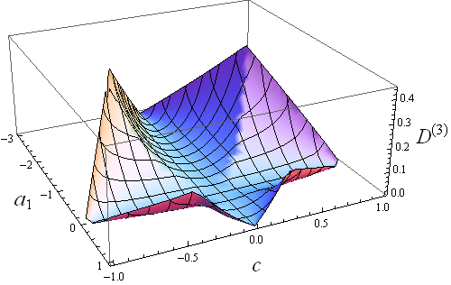
Figure 1: Genuine Tripartite Quantum Discord for $c_{1}=c_{2}=c$ (notice that the maximum value of z axis is set to 0.45 and not to 1.0 in order to make the graph more readable).

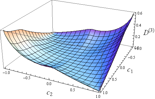
Figure 2: Genuine Tripartite Quantum Discord for $a_{1}=0$ (notice that the maximum value of z axis is set to 0.6 and not to 1.0 in order to make the graph more readable).

A further analysis of the states with $a_{1}=0$ is performed by investigating the behavior of GTQD as a function of $c_{1}$ and $c_{2}$ (see Figure 2). When $c_{1}\neq c_{2}$ the GTQD never goes to zero, and it reaches its maximum value in $(c_{1},c_{2})=(1,-1)$ or $(-1,1)$, where $D^{(3)}(\rho)=1-\frac{1}{2}\varepsilon\left(\frac{1}{\sqrt{2}}\right)$. In detail, the density matrix $\rho^{\prime}$ obtained by setting $(c_{1},c_{2})=(1,-1)$ in Eq. (17) is a linear combination of density matrices of pure GHZ states of the type:

$$\rho_{GHZ}^{\pm}(k)=\frac{1}{2}\left(\left|k\right\rangle\pm\left|\bar{k}\right\rangle\right)\left(\left\langle k\right|\pm\left\langle\bar{k}\right|\right),$$ (29)

where $k$ is a three bit binary number (from $0$ to $7$) and $\bar{k}$ is the result of flipping each bit of $k$ WEINSTEIN_ENTNGL_3Q_X . Indeed:

$$\rho^{\prime}=\frac{1}{4}\left(\rho_{GHZ}^{+}(0)+\rho_{GHZ}^{-}(1)+\rho_{GHZ}^{-}(2)+\rho_{GHZ}^{-}(3)\right),$$ (30)

and a similar expression can be found for $\rho$ when $(c_{1},c_{2})=(-1,1)$. Unlike pure GHZ states, this mixed state $\rho^{\prime}$ is not a maximally entangled one (indeed its negativity is zero, as we will see in the following), but it shows a GTQD different from zero. Moreover, also the state $\rho^{\prime\prime}$ obtained by setting $(c_{1},c_{2})=(1,1)$ is a linear combination of pure GHZ states:

$$\rho^{\prime\prime}=\frac{1}{4}\left(\rho_{GHZ}^{+}(0)+\rho_{GHZ}^{+}(1)+\rho_{GHZ}^{+}(2)+\rho_{GHZ}^{+}(3)\right),$$ (31)

but this state is characterized by zero GTQD. A similar expression can be found for $\rho$ when $(c_{1},c_{2})=(-1,-1)$, and the value of GTQD is again zero. Therefore, we conclude that a linear combinations of GHZ states is characterized by zero discord when all the states are of kind $\rho_{GHZ}^{+}(k)$ (or $\rho_{GHZ}^{-}(k)$), as it occurs for bipartite systems when we combine linearly Bell states with the same sign. Otherwise, if we combine GHZ states of kind $\rho_{GHZ}^{+}(k)$ and $\rho_{GHZ}^{-}(k)$ together, the GTQD can be different from zero.

Finally, we study $D^{(3)}(\rho)$ by setting $c_{2}=0$. We see in Figure 4 that the GTQD vanishes along the line $c_{1}=0$ and reaches its absolute maximum value (as expected) for the maximally entangled GHZ states $(a_{1},c_{1})=(3,\pm 4)$.

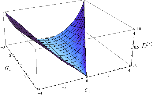
Figure 3: Genuine Tripartite Quantum Discord for $c_{2}=0$.

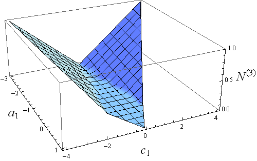
Figure 4: Tripartite Negativity for $c_{2}=0$.

Now we compare GTQD and tripartite entanglement, where the latter is quantified by means of tripartite negativity $N^{(3)}(\rho)$, given in Eq. (15). For the state of Eq. (17) we get:

$$N^{(3)}(\rho)=\frac{1}{24}\left(\left|3+a_{1}-3c_{1}\right|+\left|3+a_{1}+3c_{1}\right|+\right.$$

$$+\left.2\left|3+a_{1}-3c_{2}\right|+2\left|3+a_{1}+3c_{2}\right|+3\left|1-a_{1}-c_{2}\right|+3\left|1-a_{1}+c_{2}\right|\right)-1.$$ (32)

By evaluating this expression for some special values of the parameters $(a_{1},c_{1},c_{2})$, we see that there are regions in which the tripartite entanglement cannot be detected (i.e. the negativity is zero) but on the other hand the GTQD is different from zero. In particular, for $c_{1}=c_{2}$ or $a_{1}=0$ the tripartite negativity is zero everywhere. On the contrary, for $c_{2}=0$ (see Figure 4) there are regions where GTQD can be both smaller or larger than the negativity. This result is not surprising. Indeed, in bipartite systems for some cases entanglement has been found to be larger than quantum discord LUO_MEAS ; ANAL_QD_2QUBIT_X_states , since the latter cannot simply be considered as the sum of the entanglement and other forms of nonclassical correlations ANAL_QD_2QUBIT_X_states . However, in our case we can explain this result also on the grounds that tripartite negativity quantifies a tripartite entanglement not necessarily genuine Sabin_Trip_Negat ; EXP_MULTIP_SPINCHAIN , so it could detect in principle a larger amount of quantum correlations with respect to a genuine quantifier, such as GTQD.

6 CONCLUSIONS

In this paper, we have developed a hybrid analytical-numerical approach to find the analytical expression for GTQD $D^{(3)}(\rho)$, specifically for a subclass of X-states, symmetrical under exchange and flip of all qubits, which are defined by three parameters ($a_{1}$, $c_{1}$ and $c_{2}$). The expression of $D^{(3)}(\rho)$ depends on the relative entropy $S(\rho_{A|BC})$, whose estimation requires the minimization of the function $S_{rel}(\theta_{1},\theta_{2},\phi_{1},\phi_{2})$ depending on 4 angular variables. Numerical calculations show that $S_{rel}$ possesses only three different minimum points, which should correspond to three distinct analytical expressions for $S(\rho_{A|BC})$. Further analytical studies performed over a simplified form of $S_{rel}(\theta_{1},\theta_{2},\phi_{1},\phi_{2})$ allowed us to find the exact analytical expressions for $S(\rho_{A|BC})$ and the conditions under which they can be used. These analytical findings have been compared with some thousand of numerical simulations and have been proven always right. Moreover, they are able to reproduce the known results for GTQD in some simple systems, namely GHZ and maximally mixed states. When confronted with tripartite negativity, the calculations show that there are regions in the space of the parameters ($a_{1}$, $c_{1}$ and $c_{2}$) where entanglement cannot be detected, while genuine quantum correlations (evaluated in terms of GTDQ) differ from zero.

Further possible development of this work include the analytical study of the time evolution of genuine quantum correlations (as accounted by GTQD) and the extension of the hybrid approach here developed to more general cases.

Appendix A Appendix: Relative Entropies Definition

Following Zhao et al. ZHAO_GENUIN_TRIP , we can define the relative entropy $S(\rho_{A|BC})$ for tripartite systems as:

$$S(\rho_{A|BC})=\underset{\{E_{ij}^{BC}\}}{\min}\sum_{ij}p_{ij}S(\rho_{A|E_{ij}^{BC}}),$$ (33)

where:

$$\rho_{A|E_{ij}^{BC}}=\frac{\tilde{\rho}_{A|E_{ij}^{BC}}}{p_{ij}}=\frac{1}{p_{ij}}\mathrm{Tr}_{B,C}\left[\left(I^{A}\otimes E_{ij}^{BC}\right)\rho\right],$$ (34)

$$p_{i,j}=\mathrm{Tr}_{A,B,C}\left[\left(I^{A}\otimes E_{ij}^{BC}\right)\rho\right].$$ (35)

In the previous expressions, the operators $E_{ij}^{BC}$ are positive-operator-valued measures (POVMs) that act on parties $B$ and $C$ (i.e. in the Hilbert space $\mathcal{H}_{BC}=\mathcal{H}_{B}\otimes\mathcal{H}_{C}$), and whose outcomes are labeled with two indices ($i,j$). For sake of simplicity, we will replace the global POVM $E_{ij}^{BC}$ with the external product of two local POVMs, acting separately on parties $B$ and $C$, using the same procedure given in GIROLAMI_ANAL_PROGR_DISC_2Q . Moreover, following the convention in literature H_VEDR ; ZUR_DISC ; HAMIEH_POVMs ; GIORGI_GENUIN_MULTIP ; ZHAO_GENUIN_TRIP ), we use orthogonal projection-valued measures (PVMs) to optimize entropy in Eq. (33), since they are easier to implement in the numerical minimization process . Then, the measurement operators are:

$$E_{ij}^{BC} \rightarrow\Pi_{i}^{B}\otimes\Pi_{j}^{C}=\left|\beta_{i}\right\rangle\left\langle\beta_{i}\right|\otimes\left|\gamma_{j}\right\rangle\left\langle\gamma_{j}\right|,$$ (36)

where $\left|\beta_{i}\right\rangle$ and $\left|\gamma_{j}\right\rangle$ are orthogonal normalized basis states of the Hilbert spaces $\mathcal{H}_{B}$ and $\mathcal{H}_{C}$, respectively.

A possible parametrization of the basis vectors $\left|\beta_{i}\right\rangle$ and $\left|\gamma_{j}\right\rangle$ with respect to the standard basis $\{\left|0\right\rangle,\left|1\right\rangle\}$ can be found in literature (see FABRIZIO_GENUIN ; for a full derivation of the basis vectors see ANAL_EXPR_WERN_QTRIT ):

$$\left|\beta_{1}\right\rangle =\cos\theta_{1}\left|0_{B}\right\rangle+e^{+i\phi_{1}}\sin\theta_{1}\left|1_{B}\right\rangle,$$ (37)

$$\left|\beta_{2}\right\rangle =\sin\theta_{1}\left|0_{B}\right\rangle-e^{+i\phi_{1}}\cos\theta_{1}\left|1_{B}\right\rangle,$$ (38)

$$\left|\gamma_{1}\right\rangle =\cos\theta_{2}\left|0_{C}\right\rangle+e^{+i\phi_{2}}\sin\theta_{2}\left|1_{C}\right\rangle,$$ (39)

$$\left|\gamma_{2}\right\rangle =\sin\theta_{2}\left|0_{C}\right\rangle-e^{+i\phi_{2}}\cos\theta_{2}\left|1_{C}\right\rangle,$$ (40)

where the angles $\theta_{i}$ and $\phi_{i}$ belong to the interval $[0;2\pi)$.

Since we are studying a system whose state is symmetrical under any permutation of its subsystems, any subscript or superscript referring to a particular subsystem in the relative entropy expression (33) can be dropped. Now, recalling the sum rule $\sum_{l=1}^{2}\tilde{\lambda}_{l}^{(ij)}=p_{ij}$ for the eigenvalues $\tilde{\lambda}_{l}^{(ij)}$ of $\tilde{\rho}_{ij}=\tilde{\rho}_{A|E_{ij}^{BC}}$ (crf. Eqs. (34) and (35)), we can simplify Eq. (33) as follows:

$$S(\rho_{A|BC})=\underset{\{E_{ij}^{BC}\}}{\min}\left[-H(p)+\sum_{i,j}S(\tilde{\rho}_{ij})\right],$$ (41)

where $H(p)=-\sum_{i,j}p_{ij}\log_{2}(p_{ij})$ is the Shannon Entropy of the probability ensemble$\{p_{ij}\}$.

Now, using Eqs. (37)-(40) to write the PVMs - together with the change of variables ($\phi_{1}-\phi_{2}\rightarrow\phi_{1}$, $\phi_{1}+\phi_{2}\rightarrow\phi_{2}$), which simplifies our calculations - the relative entropy in (41) can be written as a function of four angular variables:

$$S(\rho_{A|BC}) =\underset{\theta_{i},\phi_{i}}{\min}\,S_{rel}(\theta_{1},\theta_{2},\phi_{1},\phi_{2}).$$ (42)

The final expression for $S(\rho_{A|BC})$, with all terms written explicitly, is given in Section 4.2.

Appendix B Appendix: Analytical study of $S_{rel}(\theta_{1},\theta_{2},\phi_{1},\phi_{2})$

The relative entropy $S_{rel}(\theta_{1},\theta_{2},\phi_{1},\phi_{2})$ of Eq. (22)

$$S_{rel}(\theta_{1},\theta_{2},\phi_{1},\phi_{2})=1+\frac{1}{6}\left[\lambda_{A}\log_{2}\lambda_{A}+\lambda_{B}\log_{2}\lambda_{B}\right]-\frac{1}{12}\sum_{i=1}^{4}\lambda_{i}\log_{2}\lambda_{i}$$ (43)

can be studied in a simplified form setting $\theta_{1}=\theta_{2}=\theta$. Under this condition, the $\lambda_{j}$ of Eqs. (23) become:

$$\lambda_{A} =3+a_{1}\cos^{2}(2\theta),$$

$$\lambda_{B} =3-a_{1}\cos^{2}(2\theta),$$

$$\lambda_{C} =\frac{9}{16}\sin^{4}(2\theta)\,f(\phi_{1},\phi_{2}),$$ (44)

$$f(\phi_{1},\phi_{2}) =\left[\left(c_{1}-c_{2}\right)^{2}+4c_{2}\left(\cos(\phi_{1})+\cos(\phi_{2})\right)\left(c_{2}\cos(\phi_{1})+c_{1}\cos(\phi_{2})\right)\right]$$

$$\lambda_{1,2} =\lambda_{B}\pm\sqrt{4a_{1}^{2}\cos^{2}(2\theta)+\lambda_{C}},$$

$$\lambda_{3,4} =\lambda_{A}\pm\sqrt{\lambda_{C}}.$$

The minima of $S_{rel}$ must satisfy the equation:

$$\frac{\partial S_{rel}(\theta,\theta,\phi_{1},\phi_{2})}{\partial\theta}=0,$$ (45)

which can be rewritten as follows:

$$\frac{\partial S_{rel}}{\partial\lambda_{A}}\frac{\partial\lambda_{A}}{\partial\theta}+\frac{\partial S_{rel}}{\partial\lambda_{B}}\frac{\partial\lambda_{B}}{\partial\theta}+\sum_{i=1}^{4}\frac{\partial S_{rel}}{\partial\lambda_{i}}\frac{\partial\lambda_{i}}{\partial\theta}=0.$$ (46)

The derivatives of the $\lambda_{j}$ appearing in Eq. (46) are given by:

$$\frac{\partial\lambda_{A}}{\partial\theta} =-4a_{1}\cos(2\theta)\sin(2\theta)$$

$$\frac{\partial\lambda_{B}}{\partial\theta} =+4a_{1}\cos(2\theta)\sin(2\theta)$$

$$\frac{\partial\lambda_{C}}{\partial\theta} =\frac{9}{2}\sin^{3}(2\theta)\cos(2\theta)f(\phi_{1},\phi_{2})$$ (47)

$$\frac{\partial\lambda_{1,2}}{\partial\theta} =\frac{\partial\lambda_{B}}{\partial\theta}\pm\frac{16a_{1}^{2}\cos(2\theta)\sin(2\theta)+\frac{\partial\lambda_{C}}{\partial\theta}}{2\sqrt{4a_{1}^{2}\cos^{2}(2\theta)+\lambda_{C}},},$$

$$\frac{\partial\lambda_{3,4}}{\partial\theta} =\frac{\partial\lambda_{A}}{\partial\theta}\pm\frac{\frac{\partial\lambda_{C}}{\partial\theta}}{2\sqrt{\lambda_{C}},}$$

and furthermore:

$$\frac{\partial S_{rel}}{\partial\lambda_{A,B}} =+\frac{1}{6\ln 2}(\ln\lambda_{A,B}+1)$$ (48)

$$\frac{\partial S_{rel}}{\partial\lambda_{i}} =-\frac{1}{12\ln 2}(\ln\lambda_{i}+1)\quad(i=1,2,3,4)$$ (49)

Eq. (46) then becomes:

$$\cos(2\theta)\sin(2\theta)\left[-4a_{1}\frac{\partial S_{rel}}{\partial\lambda_{A}}+4a_{1}\frac{\partial S_{rel}}{\partial\lambda_{B}}+\right.\\ \left(4a_{1}+\frac{16a_{1}^{2}+\frac{9}{2}\sin^{2}(2\theta)f(\phi_{1},\phi_{2})}{2\sqrt{4a_{1}^{2}\cos^{2}(2\theta)+\lambda_{C}},}\right)\frac{\partial S_{rel}}{\partial\lambda_{1}}+\left(4a_{1}-\frac{16a_{1}^{2}+\frac{9}{2}\sin^{2}(2\theta)f(\phi_{1},\phi_{2})}{2\sqrt{4a_{1}^{2}\cos^{2}(2\theta)+\lambda_{C}},}\right)\frac{\partial S_{rel}}{\partial\lambda_{2}}+\\ \left.\left(-4a_{1}+\frac{\frac{9}{2}\sin^{2}(2\theta)f(\phi_{1},\phi_{2})}{2\sqrt{\lambda_{C}},}\right)\frac{\partial S_{rel}}{\partial\lambda_{3}}+\left(-4a_{1}-\frac{\frac{9}{2}\sin^{2}(2\theta)f(\phi_{1},\phi_{2})}{2\sqrt{\lambda_{C}},}\right)\frac{\partial S_{rel}}{\partial\lambda_{4}}\right]=0$$ (50)

This expression shows that $\frac{\partial S_{rel}}{\partial\theta}=0$ when $\sin(2\theta)=0$ or $\cos(2\theta)=0$, that is the function can attain its minimum value for a value in the set $\theta=0+k\frac{\pi}{2}$ or $\theta=\frac{\pi}{4}+k\frac{\pi}{2}$, where $k\in\mathbb{Z}$. Indeed, it can be shown that the whole l.h.s. of Eq. (50) goes to zero when $\theta$ approaches in the limit the values listed before.

When we make the further assumption that $\theta=\frac{\pi}{4}$ and $\phi_{1}=0$ (as suggested by numerical calculations), we get:

$$\lambda_{A} =3,$$

$$\lambda_{B} =3,$$

$$\lambda_{C} =\frac{9}{16}\,f(0,\phi_{2}),$$ (51)

$$f(0,\phi_{2}) =\left[\left(c_{1}-c_{2}\right)^{2}+4c_{2}\left(1+\cos(\phi_{2})\right)\left(c_{2}+c_{1}\cos(\phi_{2})\right)\right],$$

$$\lambda_{1,2} =\lambda_{3,4}=3\pm\sqrt{\lambda_{C}},$$

and

$$S_{rel}({\textstyle\frac{\pi}{4}},{\textstyle\frac{\pi}{4}},0,\phi_{2})=1+\log_{2}3-\frac{1}{6}\sum_{i=1}^{2}\lambda_{i}\log_{2}\lambda_{i}.$$ (52)

Therefore, the minimum is reached when

$$\frac{\partial S_{rel}({\textstyle\frac{\pi}{4}},{\textstyle\frac{\pi}{4}},0,\phi_{2})}{\partial\phi_{2}}=0,$$ (53)

that is

$$\frac{\partial}{\partial\phi_{2}}\left(\lambda_{1}\log_{2}\lambda_{1}+\lambda_{2}\log_{2}\lambda_{2}\right)=0.$$ (54)

With further simplifications we get:

$$\left[\ln\frac{\left(3+\sqrt{\lambda_{C}}\right)}{\left(3-\sqrt{\lambda_{C}}\right)}\frac{1}{2\ln 2\sqrt{\lambda_{C}}}\right]\frac{\partial\lambda_{C}}{\partial\phi_{2}}=0.$$ (55)

The expression in the square brackets is always greater than 0, since the argument of the logarithm is always greater than 1 if $\lambda_{C}>0$, and when $\lambda_{C}\rightarrow 0$ the limit is finite, positive and different from zero. Therefore the extremum can be found only for:

$$\frac{\partial\lambda_{C}}{\partial\phi_{2}}=0\quad\Longleftrightarrow\quad\frac{\partial f(0,\phi_{2})}{\partial\phi_{2}}=0,$$ (56)

which leads to the final equation:

$$\sin(\phi_{2})\left(c_{2}+c_{1}+2c_{1}\cos(\phi_{2})\right)=0.$$ (57)

The solutions are:

$$\sin(\phi_{2})=0\quad\text{or}\quad\cos(\phi_{2})=\left(-\frac{c_{1}+c_{2}}{2c_{1}}\right),$$ (58)

that is

$$\phi_{2}=0+k\pi\quad\text{or}\quad\phi_{2}=\pm\arccos\left(-\frac{c_{1}+c_{2}}{2c_{1}}\right)+2k\pi,$$ (59)

where $k\in\mathbb{Z}$. Clearly, the second set of extrema exists only if:

$$-1\leq-\frac{c_{1}+c_{2}}{2c_{1}}\leq+1\quad\Rightarrow\quad\begin{cases}c_{1}>0\quad\textrm{and}\quad&-3c_{1}\leq c_{2}\leq c_{1}\\ c_{1}<0\quad\textrm{and}\quad&c_{1}\leq c_{2}\leq-3c_{1}\end{cases}.$$ (60)

Appendix C Appendix: Comparison between $S_{2}$ and $S_{3}$

When $\theta={\textstyle\frac{\pi}{4}}$ and $\phi_{1}=0$, the expression for $S_{rel}$ can be written as:

$$S_{rel}({\textstyle\frac{\pi}{4}},{\textstyle\frac{\pi}{4}},0,\phi_{2}) =1+\log_{2}3-\frac{1}{6}\left[\left(3+\sqrt{\lambda_{C}}\right)\log_{2}\left(3+\sqrt{\lambda_{C}}\right)+\left(3-\sqrt{\lambda_{C}}\right)\log_{2}\left(3-\sqrt{\lambda_{C}}\right)\right]$$

$$=1-\frac{1}{2}\left[\left(1+\frac{1}{3}\sqrt{\lambda_{C}}\right)\log_{2}\left(1+\frac{1}{3}\sqrt{\lambda_{C}}\right)+\left(1-\frac{1}{3}\sqrt{\lambda_{C}}\right)\log_{2}\left(1-\frac{1}{3}\sqrt{\lambda_{C}}\right)\right]$$

$$=1-\frac{1}{2}\varepsilon\left(\frac{1}{3}\sqrt{\lambda_{C}}\right),$$ (61)

where $\varepsilon(x)$ is given by (26). The function $S(x)=1-\frac{1}{2}\varepsilon(x)$ is known in the literature as an estimator of correlations and relative entropies in bipartite systems LUO_QBIT , and its expression holds only for $-1\leq x\leq 1$ (in our case it is always $x>0$). Due to its symmetry properties, $S(x)$ has its maximum value for $x=0$, and decreases monotonically as $x$ approaches $1$ (or $-1$). Therefore we conclude that:

$$S(x_{1})<S(x_{2})\Longleftrightarrow x_{1}>x_{2}\quad\forall x_{1},x_{2}\geq 0$$ (62)

If $\phi_{2}=0$, then $\lambda_{C}$ takes the following value:

$$\lambda_{C}=\frac{9}{16}\,f(0,0)=\frac{9}{16}(3c_{2}+c_{1})^{2},$$ (63)

and the corresponding expression for $S_{rel}$ is:

$$S_{2}=S_{rel}({\textstyle\frac{\pi}{4}},{\textstyle\frac{\pi}{4}},0,0)=1-\frac{1}{2}\varepsilon\left(\frac{|3c_{2}+c_{1}|}{4}\right)=1-\frac{1}{2}\varepsilon\left(\frac{3c_{2}+c_{1}}{4}\right)$$ (64)

The $\lambda_{C}$ expression for $\phi_{2}=\bar{\phi}_{2}=\arccos\left(-\frac{c_{1}+c_{2}}{2c_{1}}\right)$ is the following one:

$$\lambda_{C}=\frac{9}{16}\,f(0,\bar{\phi}_{2})=\frac{9}{16}\frac{\left(c_{1}-c_{2}\right)^{3}}{c_{1}},$$ (65)

which appears under a square root (for a real eigenvalue), and therefore is acceptable only if:

$$\frac{\left(c_{1}-c_{2}\right)}{c_{1}}\geq 0\quad\Rightarrow\quad\begin{cases}c_{1}\geq c_{2}&\textrm{if}\;c_{1}>0\\ c_{1}\leq c_{2}.&\textrm{if}\;c_{1}<0\end{cases}.$$ (66)

The corresponding expression for $S_{rel}$ becomes:

$$S_{3}=S_{rel}({\textstyle\frac{\pi}{4}},{\textstyle\frac{\pi}{4}},0,\bar{\phi}_{2})=1-\frac{1}{2}\varepsilon\left({\textstyle\frac{1}{4}\sqrt{\frac{\left(c_{1}-c_{2}\right)^{3}}{c_{1}}}}\right)$$ (67)

When both $S_{2}$ and $S_{3}$ expressions are well defined (see Eq. (24)), then the absolute minimum of $S_{rel}$ can occur only in the lowest of these two values, and according to Eq. (62) we conclude that

$$S_{3}<S_{2}\Longleftrightarrow\frac{\left(c_{1}-c_{2}\right)^{3}}{c_{1}}>(3c_{2}+c_{1})^{2}\Longleftrightarrow c_{1}\cdot c_{2}<0.$$ (68)

Now, collecting together the last Eq. (68) and the existence conditions for $S_{3}$ (Eqs. (60) and (66)) we conclude that:

$$S_{3}<S_{2}\Longleftrightarrow c_{1}\cdot c_{2}<0\quad\textrm{and}\quad|c_{2}|\leq|3c_{1}|.$$ (69)

References

- (1) A. Datta, S.T. Flammia, C.M. Caves, Phys. Rev. A 72, 042316 (2005). DOI 10.1103/PhysRevA.72.042316. URL http://link.aps.org/doi/10.1103/PhysRevA.72.042316
- (2) A. Datta, G. Vidal, Phys. Rev. A 75, 042310 (2007). DOI 10.1103/PhysRevA.75.042310. URL http://link.aps.org/doi/10.1103/PhysRevA.75.042310
- (3) A. Datta, A. Shaji, C.M. Caves, Phys. Rev. Lett. 100, 050502 (2008). DOI 10.1103/PhysRevLett.100.050502. URL http://link.aps.org/doi/10.1103/PhysRevLett.100.050502
- (4) B.P. Lanyon, M. Barbieri, M.P. Almeida, A.G. White, Phys. Rev. Lett. 101, 200501 (2008). DOI 10.1103/PhysRevLett.101.200501. URL http://link.aps.org/doi/10.1103/PhysRevLett.101.200501
- (5) M.A. Nielsen, I.L. Chuang, Quantum Computation and Quantum Information (Cambridge University Press, Cambridge, 2000)
- (6) R. Horodecki, P. Horodecki, M. Horodecki, K. Horodecki, Rev. Mod. Phys. 81, 865 (2009). DOI 10.1103/RevModPhys.81.865. URL http://link.aps.org/doi/10.1103/RevModPhys.81.865
- (7) H. Ollivier, W.H. Zurek, Phys. Rev. Lett. 88, 017901 (2001). DOI 10.1103/PhysRevLett.88.017901. URL http://link.aps.org/doi/10.1103/PhysRevLett.88.017901
- (8) L. Henderson, V. Vedral, Journal of Physics A: Mathematical and General 34(35), 6899 (2001). URL http://stacks.iop.org/0305-4470/34/i=35/a=315
- (9) S. Luo, Phys. Rev. A 77, 042303 (2008). DOI 10.1103/PhysRevA.77.042303. URL http://link.aps.org/doi/10.1103/PhysRevA.77.042303
- (10) S. Luo, Phys. Rev. A 77, 022301 (2008). DOI 10.1103/PhysRevA.77.022301. URL http://link.aps.org/doi/10.1103/PhysRevA.77.022301
- (11) D. Girolami, G. Adesso, Phys. Rev. A 83, 052108 (2011). DOI 10.1103/PhysRevA.83.052108. URL http://link.aps.org/doi/10.1103/PhysRevA.83.052108
- (12) S. Javad Akhtarshenas, H. Mohammadi, F.S. Mousavi, V. Nassajpour, arXiv:1304.3914 (2013). URL http://arxiv.org/abs/1304.3914
- (13) C.H. Bennett, A. Grudka, M. Horodecki, P. Horodecki, R. Horodecki, Phys. Rev. A 83, 012312 (2011). DOI 10.1103/PhysRevA.83.012312. URL http://link.aps.org/doi/10.1103/PhysRevA.83.012312
- (14) C.C. Rulli, M.S. Sarandy, Phys. Rev. A 84, 042109 (2011). DOI 10.1103/PhysRevA.84.042109. URL http://link.aps.org/doi/10.1103/PhysRevA.84.042109
- (15) J. Xu, Physics Letters A 377(3–4), 238 (2013). DOI http://dx.doi.org/10.1016/j.physleta.2012.11.054. URL http://www.sciencedirect.com/science/article/pii/S0375960112012339
- (16) I. Chakrabarty, P. Agrawal, A. Pati, The European Physical Journal D 65(3), 605 (2011). DOI 10.1140/epjd/e2011-20543-y. URL http://dx.doi.org/10.1140/epjd/e2011-20543-y
- (17) G.L. Giorgi, B. Bellomo, F. Galve, R. Zambrini, Phys. Rev. Lett. 107, 190501 (2011). DOI 10.1103/PhysRevLett.107.190501. URL http://link.aps.org/doi/10.1103/PhysRevLett.107.190501
- (18) S. Vinjanampathy, A.R.P. Rau, Journal of Physics A: Mathematical and Theoretical 45(9), 095303 (2012). URL http://stacks.iop.org/1751-8121/45/i=9/a=095303
- (19) Y. Huang, New Journal of Physics 16(3), 033027 (2014). URL http://stacks.iop.org/1367-2630/16/i=3/a=033027
- (20) F. Buscemi, P. Bordone, Phys. Rev. A 87, 042310 (2013). DOI 10.1103/PhysRevA.87.042310. URL http://link.aps.org/doi/10.1103/PhysRevA.87.042310
- (21) J. Maziero, F.M. Zimmer, Phys. Rev. A 86, 042121 (2012). DOI 10.1103/PhysRevA.86.042121. URL http://link.aps.org/doi/10.1103/PhysRevA.86.042121
- (22) A.L. Grimsmo, S. Parkins, B.S.K. Skagerstam, Phys. Rev. A 86, 022310 (2012). DOI 10.1103/PhysRevA.86.022310. URL http://link.aps.org/doi/10.1103/PhysRevA.86.022310
- (23) J.T. Cai, A. Abliz, Physica A: Statistical Mechanics and its Applications 392(10), 2607 (2013). DOI http://dx.doi.org/10.1016/j.physa.2013.01.041. URL http://www.sciencedirect.com/science/article/pii/S0378437113000939
- (24) L. Qiu, G. Tang, X. qing Yang, A. min Wang, EPL (Europhysics Letters) 105(3), 30005 (2014). URL http://stacks.iop.org/0295-5075/105/i=3/a=30005
- (25) Y.S. Weinstein, Phys. Rev. A 79, 012318 (2009). DOI 10.1103/PhysRevA.79.012318. URL http://link.aps.org/doi/10.1103/PhysRevA.79.012318
- (26) Y.S. Weinstein, Phys. Rev. A 82, 032326 (2010). DOI 10.1103/PhysRevA.82.032326. URL http://link.aps.org/doi/10.1103/PhysRevA.82.032326
- (27) M. Ali, A.R.P. Rau, G. Alber, Phys. Rev. A 81, 042105 (2010). DOI 10.1103/PhysRevA.81.042105. URL http://link.aps.org/doi/10.1103/PhysRevA.81.042105
- (28) X.M. Lu, J. Ma, Z. Xi, X. Wang, Phys. Rev. A 83, 012327 (2011). DOI 10.1103/PhysRevA.83.012327. URL http://link.aps.org/doi/10.1103/PhysRevA.83.012327
- (29) Q. Chen, C. Zhang, S. Yu, X.X. Yi, C.H. Oh, Phys. Rev. A 84, 042313 (2011). DOI 10.1103/PhysRevA.84.042313. URL http://link.aps.org/doi/10.1103/PhysRevA.84.042313
- (30) Y. Huang, Phys. Rev. A 88, 014302 (2013). DOI 10.1103/PhysRevA.88.014302. URL http://link.aps.org/doi/10.1103/PhysRevA.88.014302
- (31) V. Vedral, Rev. Mod. Phys. 74, 197 (2002). DOI 10.1103/RevModPhys.74.197. URL http://link.aps.org/doi/10.1103/RevModPhys.74.197
- (32) K. Modi, T. Paterek, W. Son, V. Vedral, M. Williamson, Phys. Rev. Lett. 104, 080501 (2010). DOI 10.1103/PhysRevLett.104.080501. URL http://link.aps.org/doi/10.1103/PhysRevLett.104.080501
- (33) M. Okrasa, Z. Walczak, Europhys. Lett. 96(6), 60003 (2011). URL http://stacks.iop.org/0295-5075/96/i=6/a=60003
- (34) G. Vidal, R.F. Werner, Phys. Rev. A 65, 032314 (2002). DOI 10.1103/PhysRevA.65.032314. URL http://link.aps.org/doi/10.1103/PhysRevA.65.032314
- (35) C. Sabín, G. García-Alcaine, The European Physical Journal D 48(3), 435 (2008). DOI 10.1140/epjd/e2008-00112-5. URL http://dx.doi.org/10.1140/epjd/e2008-00112-5
- (36) V. Coffman, J. Kundu, W.K. Wootters, Phys. Rev. A 61, 052306 (2000). DOI 10.1103/PhysRevA.61.052306. URL http://link.aps.org/doi/10.1103/PhysRevA.61.052306
- (37) W. Dür, G. Vidal, J.I. Cirac, Phys. Rev. A 62, 062314 (2000). DOI 10.1103/PhysRevA.62.062314. URL http://link.aps.org/doi/10.1103/PhysRevA.62.062314
- (38) T. Yu, J.H. Eberly, Phys. Rev. Lett. 93, 140404 (2004). DOI 10.1103/PhysRevLett.93.140404. URL http://link.aps.org/doi/10.1103/PhysRevLett.93.140404
- (39) G.L. Giorgi, S. Campbell, arXiv:1409.1021 (2014)
- (40) B. Ye, Y. Liu, J. Chen, X. Liu, Z. Zhang, Quantum Information Processing 12(7), 2355 (2013). DOI 10.1007/s11128-013-0531-y. URL http://dx.doi.org/10.1007/s11128-013-0531-y
- (41) L. Zhao, X. Hu, R.H. Yue, H. Fan, Quantum Information Processing pp. 1–13 (2013). DOI 10.1007/s11128-013-0525-9. URL http://dx.doi.org/10.1007/s11128-013-0525-9
- (42) S. Hamieh, R. Kobes, H. Zaraket, Phys. Rev. A 70, 052325 (2004). DOI 10.1103/PhysRevA.70.052325. URL http://link.aps.org/doi/10.1103/PhysRevA.70.052325